A Characteristic Particle Length.

Abstract

It is argued that there are characteristic intervals associated with any particle that can be derived without reference to the speed of light $c$. Such intervals are inferred from zeros of wavefunctions which are solutions to the Schrödinger equation. The characteristic lenght is $\ell=\beta^{2}\hbar^{2}/(8Gm^{3})$, where $\beta=3.8\dots$; this lenght might lead to obsevational effects on objects the size of a virus.

1 Introduction.

Consider the spreading of the wave-packet in non-relativistic quantum mechanics. One can ask at what point does gravitational attraction stop its spreading, compare [4] where it was asked whether the deviation of geodesics and wave spreading could cancel; however as it stands the wave-packet is a solution to Schrödinger’s equation [5]eq.6.16

$$i\hbar\frac{\partial\psi}{\partial t}=-\frac{\hbar^{2}}{2m}\nabla\psi+V\psi,$$ (1)

and so obeys Ehrenfest’s theorem [5]eq.7.10

$$\frac{d}{dt}<p_{a}>=-\left<V_{,a}\right>,$$ (2)

but the potential $V$ was taken to vanish in the derivation of the wavefunction so that gravitational attraction cannot be taken into account. To overcome this one has to start again and derive the wavefunction with a non-vanishing gravitational potential from the beginning .

Non-relativistic quantum mechanics and newtonian gravity are also used to describe the cow experiment [3]. Here throughout charge and spin are ignored although for most particles this is a big assumption, this is done for reasons of simplicity. The conventions used are: a wavefunction is any solution to the Schrödinger equation, a wave-packet is a wavefuntion with a distribution which has a well-defined mean and variance, signature $-,+,+,+$. The use of $d$ is avoided as it can both denote distance and dimension, $n$ is used to denote the number of spatial dimensions. It turns out that $n=1,2,4$ are all exceptional cases, so to avoid equation clutter we usually stick to $d=3$ unless stated otherwise. Some constants, see [1], used are: first zero of the Bessel J function $\beta=3.831705970$, Euler’s constant $\gamma=0.5772156649$, Planck’s constant divided by $2\pi$ $\hbar=1.054571726(47)\times 10^{-34}Js$, gravitational constant $G=6.67384(80)\times 10^{-11}m^{3}kg^{-1}s^{-2}$, speed of light $c=2.99792458\times 10^{8}ms^{-1}$. The Planck units are

$$m_{p}\equiv\sqrt{\frac{\hbar c}{G}},~{}~{}~{}l_{p}\equiv\sqrt{\frac{\hbar G}{c^{3}}},~{}~{}~{}t_{p}\equiv\sqrt{\frac{\hbar G}{c^{5}}}.$$ (3)

2 Static Case.

Taking the time independent Schrödinger equation, (1) with vanishing LHS, and with vanishing potential $V=0$, the spherically symmetric solution is

$$\psi(r)=A+\frac{B}{r},$$ (4)

where $A$ and $B$ are amplitude constants. Now taking the Newtonian gravitational potential

$$V=-\frac{GM{\tt m}}{r},$$ (5)

equating the Schrödinger mass $m$, the gravitating mass $M$ and the test mass ${\tt m}$ and using the notation

$$k\equiv\frac{2Gm^{3}}{\hbar^{2}},$$ (6)

where $k$ is of dimensions $L^{-1}$, the time independent spherically symmetric Schrödinger equations becomes

$$0=\psi_{rr}+\frac{2}{r}\psi_{r}+\frac{k}{r}\psi,$$ (7)

which is a Bessel equation with solution

$$\psi(r)=\frac{C}{\surd r}BesselJ(1,2\sqrt{kr})+\frac{D}{\surd r}BesselY(1,2\sqrt{kr}),$$ (8)

where $C$ and $D$ are amplitude constants, see the figure.

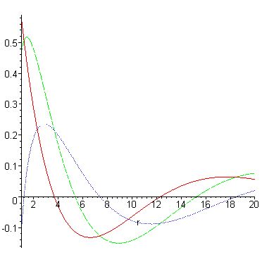
Figure 1: $BesselJ(1,2\sqrt{(}r))/\sqrt{(}r)$, $BesselY(1,2\sqrt{(}r))/\sqrt{(}r)$, $BesselJ(1,2\sqrt{(}r))/\sqrt{(}r)+BesselY(1,2\sqrt{(}r))/\sqrt{(}r)$

Note $\beta^{2}/4=3.67049266$ is where the intercept is. Briefly for $n=1$ (8) is replaced by trigonometric functions, for $n=2$ (4) and (5) involve logs, for $n=4$ the Bessel order and argument diverge, for $n\geq 5$ the external $\surd r\rightarrow r^{1-n/2}$, the argument $\surd r\rightarrow r^{2-n/2}$ and the order $1\rightarrow(n-2)/(4-n)$. Expanding (8) to first order in $r$ and choosing no mixing of the terms

$$A=\sqrt{r}C,~{}~{}~{}B=-\frac{D}{\pi\sqrt{k}},$$ (9)

gives the lowest order correction to (4)

$$\psi(r)=A\left[1-\frac{kr}{2}+\dots\right]+\frac{B}{r}\left[1+kr(1-2\gamma)-kr\ln(\sqrt{kr})+\dots\right].$$ (10)

At first sight this is counter intuitive as one would expect the addition of a potential to add short range decaying terms to the wavefunction; however one should think of the Schrödinger equation as a statement of the conservation of energy and gravitational energy is negative hence the increasing terms. That (8) sometimes has negative wavefunction is not necessarily unphysical as it is products $\psi\psi^{*}$ that correspond to measurable quantities. There is the question of what the zeros of $\psi$ correspond to. The solutions (4) and (8) are pre-interpretation solutions to the Schrödinger equation in the sense that one cannot construct expectations to the momenta and so forth as there is no time-dependence or overall energy: pre-interpretational can be thought of as the Schrödinger equation (1) with the LHS taken to vanish. Another way of thinking of this is that a solution (4) or (8) is a choice of vacuum, so that normally one choose only $A\neq 0$ but when self-gravitation is taken into account the simplest choice is only $C\neq 0$. Once this choice has been taken one has a critical distance where the wavefunction vanishes

$$\ell\equiv r_{crit}=\frac{\beta^{2}}{4k}=\frac{\beta^{2}\hbar^{2}}{8Gm^{3}}.$$ (11)

3 Non-static Case.

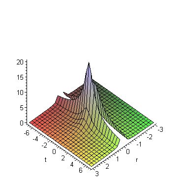
Figure 2: Matterhorn of A and B amplitudes both non-vanishing

In the non-static case there is the time dependent Gaussian wave-packet solution is

$$\psi(r,t)=\left[A+B\left(\frac{r}{f(t)}\right)^{(2-n)}\right]f(t)^{-\frac{n}{2}}\exp\left(-\frac{r^{2}}{2f(t)\sigma^{2}}\right)$$ (12)

where $f(t)\equiv 1+i\hbar t/(m\sigma^{2})$, $A,~{}B$ are constants as in (4), $\sigma$ is the raw variance. The $A$ term corresponds to a flat solution with a Gaussian added, the $B$ term corresponds to a reciprocal point particle potential with a Gaussian added this term diverges as $r$ goes to $0$, the terms can be added as can be checked explicitly and as would be anticipated from the superposition principle. The solution is to a $V=0$ Schrödinger equation, adding $V=-\alpha/r^{2}$ is straightforward, time dependent solutions for other potentials in particular for $V=-k/r$ are unknown. The solution can be expressed in terms of modified Whittaker functions

$$\psi(r,t)=\left[A+B\left(\frac{r}{f(t)}\right)^{(2-n)}\right]f(t)^{-\frac{n}{2}}\left(-\frac{r^{2}}{\sigma^{2}f(t)}\right)^{\alpha}{\rm WhittakerM}\{\alpha,-\alpha-1/2,-\frac{r^{2}}{\sigma^{2}f(t)}\}$$ (13)

or hypergeometric functions

$$\psi(r,t)=\left[A+B\left(\frac{r}{f(t)}\right)^{(2-n)}\right]f(t)^{-\frac{n}{2}}{\rm hypergeom}\{[-2\alpha],[-2\alpha],-\frac{r^{2}}{2\sigma^{2}f(t)}\},$$ (14)

where $\alpha$ is a constant. There does not appear to be a solution with the Gaussian distribution replaced by any Pearson distribution or a similar distribution, however because to the radially dependent terms in front of the gaussian there is now non-vanishing excess kurtosis, and $\sigma$ is no longer the variance which is why it is called the raw variance above. Setting $n=3,~{}~{}~{}A=B=m=\hbar=\sigma=1$ then $\psi\psi^{*}$ gives the Matterhorn shape in the figure, there is a divergence at the origin as would be expected for $B\neq 0$ because of the divergence of the reciprocal potential.

There seems to be no time dependent version of the Bessel solutions (8) or even an approximation to this. The characteristic delocation time interval in the above is

$$t_{deloc}=\frac{m\sigma^{2}}{\hbar},$$ (15)

usually the raw variance $\sigma$ is taken to be a hand chosen delocalization length; however taking it to be $\ell$ given by (11) gives the characteristic time

$$\tau=\frac{\beta^{4}\hbar^{3}}{64G^{2}m^{5}}.$$ (16)

4 Conclusion.

The critical lengths and times for typical masses are given in the table below: for elementary particles they are too long to be measured whereas for astronomical sized particles they are too short to be observed, in both cases any effect would be masked by other factors; however for objects the size of a virus there is a possibility of a measurable effect. The long range for elementary particles might suggest that they have an effect in the ’next’ universe, see [2], however relativistic cosmology has the speed of light built into it from the beginning so that the critical length (11) is not really applicable.

The static generalization of (8) to the Klein-Gordon equation is immediate as the time derivative terms do not enter; however in the time dependent case generalization of (12) to the Klein-Gordon equation is unlikely to have a similar form as (12) has single powers of $\hbar$ which do not occur in the Klein-Gordon equation. No method is known to generalize to the Dirac equation.

Comparison can be made between the values in the table and other known radii: the classical electron radius is $r_{e}=e^{2}/(mc^{2})=3\times 10^{-15}m$ and the Bohr radius is $a_{0}=(4\pi\epsilon_{0}\hbar^{2})/((m_{e}e^{2})=5\times 10^{-11}m$, both of which are of orders of magnitude different from the values of $\ell$ in the table below. Note that the denominator of the Bohr radius is of similar form to (11) when $e\rightarrow m$. These radii govern lattice spacings and cross sections, but it is not clear what if anything is a lattice dependent on $\ell$ or how cross sections could depend on it; presumably any lattice spacing would be about the size of a virus which is larger than usual.

Using the Compton wavelength $r_{c}=\hbar/(mc)$, the Schwarzschild radius $r_{s}=(2Gm)/c^{2}$, Planck units (3), the critical length (11) and the critical time (16), it is possible to produce the dimensionless ratios

$$\frac{r_{s}}{r_{c}}=2\left(\frac{m}{m_{p}}\right)^{2},~{}\frac{r_{c}}{\ell}=\frac{8}{\beta^{2}}\left(\frac{m}{m_{p}}\right)^{2},~{}\frac{r_{s}}{\ell}=\frac{16}{\beta^{2}}\left(\frac{m}{m_{p}}\right)^{4},~{}\frac{t_{p}}{\tau}=\frac{64}{\beta^{4}}\left(\frac{m}{m_{p}}\right)^{5},$$ (17)

which shows that the are no new dimensionless quantities except the universal mathematical constant $\beta$, the only dimensionless quantity which takes a different value for each particle is the mass in Planck units.

Table of Characteristic Quantities.

$$\begin{array}[]{llll}{\rm Particle}&{\rm Mass~{}in~{}Kg.}&{\rm Distance~{}\ell~{}in~{}meters}&{\rm Time~{}\tau~{}in~{}seconds}\\ {\rm Electron}&9\times 10^{-31}&~{}~{}~{}~{}~{}~{}4\times 10^{32}&2\times 10^{69}\\ {\rm Proton}&2\times 10^{-27}&~{}~{}~{}~{}~{}~{}3\times 10^{22}&3\times 10^{52}\\ {\rm Lead~{}atom}&4\times 10^{-25}&~{}~{}~{}~{}~{}~{}5\times 10^{15}&9\times 10^{40}\\ {\rm Buckyball~{}molecule}&1\times 10^{-24}&~{}~{}~{}~{}~{}~{}3\times 10^{14}&9\times 10^{38}\\ {\rm Protein}&6\times 10^{-23}&~{}~{}~{}~{}~{}~{}1\times 10^{9}&1\times 10^{30}\\ {\rm Haemoglobin}&1\times 10^{-22}&~{}~{}~{}~{}~{}~{}3\times 10^{8}&9\times 10^{28}\\ {\rm DNA}&2\times 10^{-21}&~{}~{}~{}~{}~{}~{}4\times 10^{4}&3\times 10^{22}\\ {\rm Small~{}virus}&7\times 10^{-20}&~{}~{}~{}~{}~{}~{}9\times 10^{-1}&5\times 10^{14}\\ {\rm Large~{}virus}&1\times 10^{-17}&~{}~{}~{}~{}~{}~{}3\times 10^{-7}&9\times 10^{3}\\ {\rm Bacteria}&9\times 10^{-16}&~{}~{}~{}~{}~{}~{}4\times 10^{-13}&2\times 10^{-6}\\ {\rm Yeast}&6\times 10^{-14}&~{}~{}~{}~{}~{}~{}4\times 10^{-17}&3\times 10^{-13}\\ {\rm Man}&9\times 10^{1}&~{}~{}~{}~{}~{}~{}4\times 10^{-64}&2\times 10^{-91}\\ {\rm Earth}&6\times 10^{24}&~{}~{}~{}~{}~{}~{}1\times 10^{-132}&1\times 10^{-205}\\ {\rm Sun}&2\times 10^{30}&~{}~{}~{}~{}~{}~{}4\times 10^{-148}&3\times 10^{-233}\\ {\rm Galaxy}&6\times 10^{42}&~{}~{}~{}~{}~{}~{}1\times 10^{-186}&1\times 10^{-295}\\ {\rm Cluster}&1\times 10^{46}&~{}~{}~{}~{}~{}~{}3\times 10^{-196}&9\times 10^{-312}\\ \end{array}$$ (35)

5 Acknowledgement

I would like to thank Tom Kibble for discussion on some of the topics in this paper.

References

- [1] John D. Barrow (2002), The Constants of Nature, Random House, ISBN9780099286479
- [2] Bernard J. Carr (2009), Universe or Multiverse, Cambridge University Press ISBN-10:0521140692
- [3] R. Colella, A.W.Overhauser, S.A. Werner, Observation of Gravitationally induced Quantum Interference. Phys.Rev.Lett.34(1975)1472.
- [4] Mark D. Roberts, The Quantization of Geodesic Deviation. Gen.Rel.Grav. 28(1996)1385-1392.
- [5] Leonard I. Schiff (1968), Quantum Mechanics, Third Edition, McGraw-Hill ISBN 0-07-Y85643-5