Optimization Methods for Designing Sequences with Low Autocorrelation Sidelobes

Abstract

Unimodular sequences with low autocorrelations are desired in many applications, especially in the area of radar and code-division multiple access (CDMA). In this paper, we propose a new algorithm to design unimodular sequences with low integrated sidelobe level (ISL), which is a widely used measure of the goodness of a sequence’s correlation property. The algorithm falls into the general framework of majorization-minimization (MM) algorithms and thus shares the monotonic property of such algorithms. In addition, the algorithm can be implemented via fast Fourier transform (FFT) operations and thus is computationally efficient. Furthermore, after some modifications the algorithm can be adapted to incorporate spectral constraints, which makes the design more flexible. Numerical experiments show that the proposed algorithms outperform existing algorithms in terms of both the quality of designed sequences and the computational complexity.

I Introduction

Since the 1950s, digital communications engineers have sought to identify sequences whose autocorrelation sidelobes are collectively as low as possible according to some suitable measure of “goodness”. Applications of sequences with low autocorrelation sidelobes range from synchronization to code-division multiple access (CDMA) systems and also radar systems [1, 2]. Low autocorrelation can improve the detection performance of weak targets [3] in range compression radar and it is also desired for synchronization purposes in CDMA systems. Additionally, due to the limitations of sequence generation hardware components (such as the maximum signal amplitude clip of analog-to-digital converters and power amplifiers), it is usually more desirable to transmit unimodular (i.e., constant modulus) sequences to maximize the transmitted power available in the system [4].

The focus of this paper is on the design of unimodular sequences with low (aperiodic or periodic) autocorrelation sidelobes. Let $\{x_{n}\}_{n=1}^{N}$ denote the complex unimodular (without loss of generality, we will assume the modulus to be 1) sequence to be designed. The aperiodic ($r_{k}$) and periodic ($\hat{r}_{k}$) autocorrelations of $\{x_{n}\}_{n=1}^{N}$ are defined as

$$r_{k} =\sum_{n=1}^{N-k}x_{n}x_{n+k}^{*}=r_{-k}^{*},\,k=0,\ldots,N-1,$$

$$\hat{r}_{k} =\sum_{n=1}^{N}x_{n}x_{(n+k)({\rm mod}\,N)}^{*}=\hat{r}_{-k}^{*},\,k=0,\ldots,N-1.$$

Then the integrated sidelobe level (ISL) of the aperiodic autocorrelations is defined as

$${\rm ISL}=\sum_{k=1}^{N-1}|r_{k}|^{2},$$ (1)

which will be used to measure the goodness of the aperiodic autocorrelation property of a sequence. The ISL metric for the periodic autocorrelations can be defined similarly. Note that the ISL metric is highly related to another important goodness measure: the merit factor (MF), which is defined as the ratio of the central lobe energy to the total energy of all other lobes by Golay in 1972 [5], i.e.,

$${\rm MF}=\frac{\left|r_{0}\right|^{2}}{2\sum_{k=1}^{N-1}|r_{k}|^{2}}=\frac{N^{2}}{2{\rm ISL}}.$$ (2)

Owing to the practical importance and widespread applications of sequences with good autocorrelation properties, in particular with low ISL values or large MF values, a lot of effort has been devoted to identifying these sequences via either analytical construction methods or computational approaches in the literature. The studies focused more on the design of binary sequences at the early stage, and extended to polyphase sequences later; see [6, 5, 7, 8, 9, 10, 11] for the case of binary sequences and [12, 13, 14, 15, 16, 17, 18] for the case of polyphase or unimodular sequences. Some sequences with good autocorrelation properties that can be constructed in closed-form have been proposed in the literature, such as the Frank sequence [12] and the Golomb sequence [13]. Computational approaches, such as exhaustive search [8], evolutionary algorithms [9], heuristic search [11] and stochastic optimization methods [14, 15], have also been suggested. However, these methods are generally not capable of designing long sequences, say $N\sim 10^{3}$ or larger, due to the increasing computational complexity. Recently, an algorithm named CAN (cyclic algorithm new) was proposed in [17] that can be used to produce unimodular sequences of length $N\sim 10^{6}$ or even larger with low aperiodic ISL and it has been adapted to generate sequences with impulse-like periodic autocorrelations [19] and incorporate spectral constraints [20]. But rather than the original ISL metric, the CAN algorithm tries to minimize another simpler criterion which is stated to be “almost equivalent” to the ISL metric.

In this paper, we develop an efficient algorithm that directly minimizes the ISL metric (of both aperiodic and periodic autocorrelations) monotonically, which we call MISL (monotonic minimizer for integrated sidelobe level). The MISL algorithm is derived via applying the general majorization-minimization (MM) method to the ISL minimization problem twice and admits a simple closed-form solution at every iteration. The convergence of the algorithm to a stationary point is proved. Similar to the CAN algorithm, the proposed MISL algorithm can also be implemented via fast Fourier transform (FFT) operations and is thus very efficient. But due to the nature of double majorization, the MISL algorithm may converge very slow especially for large $N,$ and we propose to apply some acceleration schemes to fix this issue. A MISL-like algorithm, which shares the simplicity and efficiency of MISL, has also been developed for minimizing the ISL metric when there are additional spectral constraints.

The remaining sections of the paper are organized as follows. In Section II, the problem formulations are presented and the CAN algorithm is reviewed. In Section III, we first give a brief review of the MM framework and then the MISL algorithm is derived, followed by the convergence analysis. In Section IV, some acceleration schemes for MISL are presented and then the spectral-MISL algorithm is developed in Section V. Finally, Section VI presents some numerical examples and the conclusions are given in Section VII.

Notation: Boldface upper case letters denote matrices, boldface lower case letters denote column vectors, and italics denote scalars. $\mathbf{R}$ and $\mathbf{C}$ denote the real field and the complex field, respectively. $\mathrm{Re}(\cdot)$ and $\mathrm{Im}(\cdot)$ denote the real and imaginary part respectively. ${\rm arg}(\cdot)$ denotes the phase of a complex number. The superscripts $(\cdot)^{T}$, $(\cdot)^{*}$ and $(\cdot)^{H}$ denote transpose, complex conjugate, and conjugate transpose, respectively. $X_{i,j}$ denotes the (i-th, j-th) element of matrix $\mathbf{X}$ and $x_{i}$ denotes the i-th element of vector $\mathbf{x}$. $\mathrm{Tr}(\cdot)$ denotes the trace of a matrix. ${\rm diag}(\mathbf{X})$ is a column vector consisting of all the diagonal elements of $\mathbf{X}$. ${\rm Diag}(\mathbf{x})$ is a diagonal matrix formed with $\mathbf{x}$ as its principal diagonal. ${\rm vec}(\mathbf{X})$ is a column vector consisting of all the columns of $\mathbf{X}$ stacked. $\mathbf{I}_{n}$ denotes an $n\times n$ identity matrix.

II Problem Formulation and Existing Methods

The problem of interest is the design of a complex unimodular sequence $\{x_{n}\}_{n=1}^{N}$ that minimizes the ISL metric (of either aperiodic or periodic autocorrelations), i.e.,

$$\begin{array}[]{ll}\underset{x_{n}}{\mathsf{minimize}}&{\rm ISL}\\ \mathsf{subject\;to}&\left|x_{n}\right|=1,\,n=1,\ldots,N.\end{array}$$ (3)

In the following, we first reformulate the problem (3) for the case of aperiodic and periodic autocorrelations respectively and then briefly review two corresponding algorithms proposed in the literature.

II-A The Aperiodic Autocorrelation

It has been shown in [17] that the ISL metric of the aperiodic autocorrelations can be expressed in the frequency domain as

$${\rm ISL}=\frac{1}{4N}\sum_{p=1}^{2N}\left[\left|\sum_{n=1}^{N}x_{n}e^{-j\omega_{p}(n-1)}\right|^{2}-N\right]^{2},$$ (4)

where $\omega_{p}=\frac{2\pi}{2N}(p-1),\>p=1,\cdots,2N$. Thus, the sequence design problem (3) becomes

$$\begin{array}[]{ll}\underset{x_{n}}{\mathsf{minimize}}&{\displaystyle\sum_{p=1}^{2N}}\left[\left|{\displaystyle\sum_{n=1}^{N}}x_{n}e^{-j\omega_{p}(n-1)}\right|^{2}-N\right]^{2}\\ \mathsf{subject\;to}&\left|x_{n}\right|=1,\,n=1,\ldots,N.\end{array}$$ (5)

Let us define

$$\mathbf{x} = [x_{1},\cdots,x_{N}]^{T}$$ (6)

$$\mathbf{a}_{p} = [1,e^{j\omega_{p}},\cdots,e^{j\omega_{p}(N-1)}]^{T},\,p=1,\ldots,2N,$$ (7)

then the problem (5) can be rewritten as

$$\begin{array}[]{ll}\underset{\mathbf{x}}{\mathsf{minimize}}&{\displaystyle\sum_{p=1}^{2N}}\left[\mathbf{a}_{p}^{H}\mathbf{x}\mathbf{x}^{H}\mathbf{a}_{p}-N\right]^{2}\\ \mathsf{subject\;to}&\left|x_{n}\right|=1,\,n=1,\ldots,N.\end{array}$$ (8)

Expanding the square in the objective yields

$$\begin{array}[]{ll}\underset{\mathbf{x}}{\mathsf{minimize}}&{\displaystyle\sum_{p=1}^{2N}}\left(\left(\mathbf{a}_{p}^{H}\mathbf{x}\mathbf{x}^{H}\mathbf{a}_{p}\right)^{2}-2N\mathbf{a}_{p}^{H}\mathbf{x}\mathbf{x}^{H}\mathbf{a}_{p}+N^{2}\right)\\ \mathsf{subject\;to}&\left|x_{n}\right|=1,\,n=1,\ldots,N,\end{array}$$ (9)

where the second term in the objective can be shown to be a constant (using Parseval’s theorem), i.e., $\sum_{p=1}^{2N}\left|\mathbf{a}_{p}^{H}\mathbf{x}\right|^{2}=2N\left\|\mathbf{x}\right\|_{2}^{2}=2N^{2}.$ Thus by ignoring the constant terms, the problem can be simplified as

$$\begin{array}[]{ll}\underset{\mathbf{x}}{\mathsf{minimize}}&{\displaystyle\sum_{p=1}^{2N}}\left(\mathbf{a}_{p}^{H}\mathbf{x}\mathbf{x}^{H}\mathbf{a}_{p}\right)^{2}\\ \mathsf{subject\;to}&\left|x_{n}\right|=1,\,n=1,\ldots,N.\end{array}$$ (10)

The problem is hard to tackle, due to the quartic objective function and also the nonconvex unit-modulus constraints.

II-B The Periodic Autocorrelation

Similarly, in the periodic case, the ISL metric ${\rm ISL}=\sum_{k=1}^{N-1}|\hat{r}_{k}|^{2}$ can also be expressed in the frequency domain as [19]

$${\rm ISL}=\frac{1}{N}\sum_{p=1}^{N}\left[\left|\sum_{n=1}^{N}x_{n}e^{-j\hat{\omega}_{p}(n-1)}\right|^{2}-N\right]^{2},$$ (11)

where $\hat{\omega}_{p}=\frac{2\pi}{N}(p-1),\>p=1,\cdots,N$. By defining

$$\hat{\mathbf{a}}_{p} = [1,e^{j\hat{\omega}_{p}},\cdots,e^{j\hat{\omega}_{p}(N-1)}]^{T},\,p=1,\ldots,N,$$ (12)

the ISL minimization problem (3) in this case can be rewritten as

$$\begin{array}[]{ll}\underset{\mathbf{x}}{\mathsf{minimize}}&{\displaystyle\sum_{p=1}^{N}}\left[\hat{\mathbf{a}}_{p}^{H}\mathbf{x}\mathbf{x}^{H}\hat{\mathbf{a}}_{p}-N\right]^{2}\\ \mathsf{subject\;to}&\left|x_{n}\right|=1,\,n=1,\ldots,N.\end{array}$$ (13)

Following similar steps as in the previous subsection, the problem can be further simplified as

$$\begin{array}[]{ll}\underset{\mathbf{x}}{\mathsf{minimize}}&{\displaystyle\sum_{p=1}^{N}}\left(\hat{\mathbf{a}}_{p}^{H}\mathbf{x}\mathbf{x}^{H}\hat{\mathbf{a}}_{p}\right)^{2}\\ \mathsf{subject\;to}&\left|x_{n}\right|=1,\,n=1,\ldots,N.\end{array}$$ (14)

We note that although problem (14) looks similar to the problem (10) in the aperiodic case, it is usually a simpler task to find sequences with good periodic autocorrelation properties. In particular, in the periodic case unimodular sequences with zero ISL exist for any length $N$ [19], however it is not possible to construct unimodular sequences with exact impulse-like aperiodic autocorrelations.

II-C Existing Methods

An algorithm named CAN was proposed in [17] for designing unimodular sequences with low ISL of aperiodic autocorrelations. But instead of minimizing the ISL metric directly, i.e., solving (5), the authors proposed to solve the following simpler problem

$$\begin{array}[]{ll}\underset{x_{n},\psi_{p}}{\mathsf{minimize}}&{\displaystyle\sum_{p=1}^{2N}}\left|{\displaystyle\sum_{n=1}^{N}}x_{n}e^{-j\omega_{p}(n-1)}-\sqrt{N}e^{j\psi_{p}}\right|^{2}\\ \mathsf{subject\;to}&\left|x_{n}\right|=1,\,n=1,\ldots,N,\end{array}$$ (15)

whose objective is quadratic in $\{x_{n}\}$. Let $\mathbf{A}$ be the following $N\times 2N$ matrix:

$$\mathbf{A}=[\mathbf{a}_{1},\ldots,\mathbf{a}_{2N}],$$ (16)

then the objective function of problem (15) can be rewritten in the following more compact form:

$$\left\|\mathbf{A}^{H}\mathbf{x}-\sqrt{N}\mathbf{v}\right\|^{2},$$ (17)

where $\mathbf{v}=[e^{j\psi_{1}},\ldots,e^{j\psi_{2N}}]^{T}.$ The CAN algorithm then minimizes (17) by alternating between $\mathbf{x}$ and $\mathbf{v}$. For a given $\mathbf{x}$, the minimization of (17) with respect to $\{\psi_{p}\}$ yields

$$\psi_{p}={\rm arg}(f_{p}),\,p=1,\ldots,2N,$$ (18)

where $\mathbf{f}=\mathbf{A}^{H}\mathbf{x}$. Similarly, for a given $\mathbf{v}$, the minimizing $\mathbf{x}$ is given by

$$x_{n}=e^{j{\rm arg}(g_{n})},\,n=1,\ldots,N,$$ (19)

where $\mathbf{g}=\mathbf{A}\mathbf{v}.$ The CAN algorithm is summarized in Algorithm 1 for ease of comparison later.

0:   sequence length $N$

1:   Set $k=0$, initialize $\mathbf{x}^{(0)}$.

2:  repeat

3:      $\mathbf{f}=\mathbf{A}^{H}\mathbf{x}^{(k)}$

4:      $v_{p}=e^{j{\rm arg}(f_{p})},\,p=1,\ldots,2N$

5:      $\mathbf{g}=\mathbf{A}\mathbf{v}$

6:      $x_{n}^{(k+1)}=e^{j{\rm arg}(g_{n})},\,n=1,\ldots,N$

7:      $k\leftarrow k+1$

8:  until  convergence

Algorithm 1 The CAN algorithm proposed in [17].

It was mentioned in [17] that the problem (15) is “almost equivalent” to the original problem (5). But as the authors also pointed out, the two problems are not exactly equivalent and they may have different solutions. It is easy to see that minimizing with respect to $\{\psi_{p}\}$ in (15) leads to

$$\begin{array}[]{ll}\underset{x_{n}}{\mathsf{minimize}}&{\displaystyle\sum_{p=1}^{2N}}\left[\left|{\displaystyle\sum_{n=1}^{N}}x_{n}e^{-j\omega_{p}(n-1)}\right|-\sqrt{N}\right]^{2}\\ \mathsf{subject\;to}&\left|x_{n}\right|=1,\,n=1,\ldots,N,\end{array}$$ (20)

which is different from the original problem (5). So the point the CAN algorithm converges to is not necessary a local minimum (or even a stationary point) of the original ISL metric minimization problem. Although CAN does not directly minimize the ISL metric, in [17] the authors showed numerically that CAN could generate sequences with good correlation properties. Moreover, CAN can be implemented via FFT, thus can be used to design very long sequences.

In the periodic case, an algorithm called PeCAN was used in [19] to construct unimodular sequences with low ISL. It can be viewed as an adaptation of the CAN algorithm for the periodic case and similarly instead of minimizing the original ISL metric (11), the PeCAN algorithm considered the simpler criterion

$$\sum_{p=1}^{N}\left|\sum_{n=1}^{N}x_{n}e^{-j\hat{\omega}_{p}(n-1)}-\sqrt{N}e^{j\psi_{p}}\right|^{2},$$ (21)

where $\{\psi_{p}\}$ are auxiliary variables as in (15). It was shown numerically in [19] that PeCAN can generate almost perfect (with zero ISL) sequences from random initializations.

Although the criteria considered by CAN and PeCAN are somehow related to the original ISL metric and the performance of the two algorithms is acceptable in some situations, one may expect that directly solving the original ISL minimization problem can probably lead to better performance. In the next section, we will develop an algorithm that directly minimizes the ISL metric, while at the same time is computationally as efficient as the CAN algorithm.

III ISL Minimization via Majorization-Minimization

In this section, we first introduce the general majorization-minimization (MM) method briefly and then develop a simple algorithm for the ISL minimization problem based on the general MM scheme. In the derivation, we will focus on the aperiodic case, i.e., the problem (10), but the resulting algorithm can be readily adapted for the periodic case.

III-A The MM Method

The MM method refers to the majorization-minimization method, which is an approach to solve optimization problems that are too difficult to solve directly. The principle behind the MM method is to transform a difficult problem into a series of simple problems. Interested readers may refer to [21] and references therein for more details (recent generalizations include [22, 23]).

Suppose we want to minimize $f(\mathbf{x})$ over $\mathcal{X}\in\mathbf{C}^{n}$. Instead of minimizing the cost function $f(\mathbf{x})$ directly, the MM approach optimizes a sequence of approximate objective functions that majorize $f(\mathbf{x})$. More specifically, starting from a feasible point $\mathbf{x}^{(0)},$ the algorithm produces a sequence $\{\mathbf{x}^{(k)}\}$ according to the following update rule

$$\mathbf{x}^{(k+1)}\in\underset{\mathbf{x}\in\mathcal{X}}{\arg\min}\,\,u(\mathbf{x},\mathbf{x}^{(k)}),$$ (22)

where $\mathbf{x}^{(k)}$ is the point generated by the algorithm at iteration $k,$ and $u(\mathbf{x},\mathbf{x}^{(k)})$ is the majorization function of $f(\mathbf{x})$ at $\mathbf{x}^{(k)}$. Formally, the function $u(\mathbf{x},\mathbf{x}^{(k)})$ is said to majorize the function $f(\mathbf{x})$ at the point $\mathbf{x}^{(k)}$ provided

$$u(\mathbf{x},\mathbf{x}^{(k)}) \geq f(\mathbf{x}),\quad\forall\mathbf{x}\in\mathcal{X},$$ (23)

$$u(\mathbf{x}^{(k)},\mathbf{x}^{(k)}) = f(\mathbf{x}^{(k)}).$$ (24)

In other words, function $u(\mathbf{x},\mathbf{x}^{(k)})$ is an upper bound of $f(\mathbf{x})$ over $\mathcal{X}$ and coincides with $f(\mathbf{x})$ at $\mathbf{x}^{(k)}$.

To summarize, to minimize $f(\mathbf{x})$ over $\mathcal{X}\in\mathbf{C}^{n}$, the main steps of the majorization-minimization scheme are

1. Find a feasible point $\mathbf{x}^{(0)}$ and set $k=0.$

2. Construct a majorization function $u(\mathbf{x},\mathbf{x}^{(k)})$ of $f(\mathbf{x})$ at $\mathbf{x}^{(k)}$.

3. Let $\mathbf{x}^{(k+1)}\in\underset{\mathbf{x}\in\mathcal{X}}{\arg\min}\,\,u(\mathbf{x},\mathbf{x}^{(k)}).$

4. If some convergence criterion is met, exit; otherwise, set $k=k+1$ and go to step (2).

It is easy to show that with this scheme, the objective value is decreased monotonically at every iteration, i.e.,

$$f(\mathbf{x}^{(k+1)})\leq u(\mathbf{x}^{(k+1)},\mathbf{x}^{(k)})\leq u(\mathbf{x}^{(k)},\mathbf{x}^{(k)})=f(\mathbf{x}^{(k)}).$$ (25)

The first inequality and the third equality follow from the the properties of the majorization function, namely (23) and (24) respectively and the second inequality follows from (22). The monotonicity makes MM algorithms very stable in practice.

III-B MISL

To solve the aperiodic problem (10) via majorization-minimization, the key step is to find a majorization function of the objective such that the majorized problem is easy to solve. For that purpose we first present a simple result that will be useful when constructing the majorization function.

Lemma 1.

Let $\mathbf{L}$ be an $n\times n$ Hermitian matrix and $\mathbf{M}$ be another $n\times n$ Hermitian matrix such that $\mathbf{M}\succeq\mathbf{L}.$ Then for any point $\mathbf{x}_{0}\in\mathbf{C}^{n}$, the quadratic function $\mathbf{x}^{H}\mathbf{L}\mathbf{x}$ is majorized by $\mathbf{x}^{H}\mathbf{M}\mathbf{x}+2{\rm Re}\left(\mathbf{x}^{H}(\mathbf{L}-\mathbf{M})\mathbf{x}_{0}\right)+\mathbf{x}_{0}^{H}(\mathbf{M}-\mathbf{L})\mathbf{x}_{0}$ at $\mathbf{x}_{0}$.

Proof:

It is easy to check that the two functions are equal at point $\mathbf{x}_{0}$. Since $\mathbf{M}\succeq\mathbf{L},$ we further have

$$\,\,\mathbf{x}^{H}\mathbf{L}\mathbf{x}$$

$$= \,\,\mathbf{x}_{0}^{H}\mathbf{L}\mathbf{x}_{0}\!+\!2{\rm Re}\left((\mathbf{x}-\mathbf{x}_{0})^{H}\mathbf{L}\mathbf{x}_{0}\right)\!+\!(\mathbf{x}-\mathbf{x}_{0})^{H}\mathbf{L}(\mathbf{x}-\mathbf{x}_{0})$$

$$\leq \,\,\mathbf{x}_{0}^{H}\mathbf{L}\mathbf{x}_{0}\!+\!2{\rm Re}\left((\mathbf{x}-\mathbf{x}_{0})^{H}\mathbf{L}\mathbf{x}_{0}\right)\!+\!(\mathbf{x}-\mathbf{x}_{0})^{H}\mathbf{M}(\mathbf{x}-\mathbf{x}_{0})$$

$$= \,\,\mathbf{x}^{H}\mathbf{M}\mathbf{x}\!+\!2{\rm Re}\left(\mathbf{x}^{H}(\mathbf{L}-\mathbf{M})\mathbf{x}_{0}\right)\!+\!\mathbf{x}_{0}^{H}(\mathbf{M}-\mathbf{L})\mathbf{x}_{0}$$

for any $\mathbf{x}\in\mathbf{C}^{n}$. The proof is complete. ∎

The objective of the problem (10) is quartic with respect to $\mathbf{x}$. To find a majorization function, some reformulations are necessary. Let us define $\mathbf{X}=\mathbf{x}\mathbf{x}^{H}$ and $\mathbf{A}_{p}=\mathbf{a}_{p}\mathbf{a}_{p}^{H}$, then the problem (10) can be rewritten as

$$\begin{array}[]{ll}\underset{\mathbf{x},\mathbf{X}}{\mathsf{minimize}}&{\displaystyle\sum_{p=1}^{2N}}{\rm Tr}(\mathbf{X}\mathbf{A}_{p})^{2}\\ \mathsf{subject\;to}&\mathbf{X}=\mathbf{x}\mathbf{x}^{H}\\ &\left|x_{n}\right|=1,\,n=1,\ldots,N.\end{array}$$ (26)

Since ${\rm Tr}(\mathbf{X}\mathbf{A}_{p})={\rm vec}(\mathbf{X})^{H}{\rm vec}(\mathbf{A}_{p})$, problem (26) is just

$$\begin{array}[]{ll}\underset{\mathbf{x},\mathbf{X}}{\mathsf{minimize}}&{\rm vec}(\mathbf{X})^{H}\mathbf{\Phi}{\rm vec}(\mathbf{X})\\ \mathsf{subject\;to}&\mathbf{X}=\mathbf{x}\mathbf{x}^{H}\\ &\left|x_{n}\right|=1,\,n=1,\ldots,N,\end{array}$$ (27)

where $\mathbf{\Phi}=\sum_{p=1}^{2N}{\rm vec}(\mathbf{A}_{p}){\rm vec}(\mathbf{A}_{p})^{H}.$ We can see that the objective of (27) is a quadratic function in $\mathbf{X}$ now. Given $\mathbf{X}^{(k)}=\mathbf{x}^{(k)}\left(\mathbf{x}^{(k)}\right)^{H}$ at iteration $k$, by choosing $\mathbf{M}=\lambda_{{\rm max}}(\mathbf{\Phi})\mathbf{I}$ in Lemma 1 we know that the objective of (27) is majorized by the following function at $\mathbf{X}^{(k)}$:

$$u_{1}(\mathbf{X},\mathbf{X}^{(k)})$$ (28)

$$= \lambda_{{\rm max}}(\mathbf{\Phi}){\rm vec}(\mathbf{X})^{H}{\rm vec}(\mathbf{X})$$

$$+2{\rm Re}\left({\rm vec}(\mathbf{X})^{H}(\mathbf{\Phi}-\lambda_{{\rm max}}(\mathbf{\Phi})\mathbf{I}){\rm vec}(\mathbf{X}^{(k)})\right)$$

$$+{\rm vec}(\mathbf{X}^{(k)})^{H}(\lambda_{{\rm max}}(\mathbf{\Phi})\mathbf{I}-\mathbf{\Phi}){\rm vec}(\mathbf{X}^{(k)})$$

where $\lambda_{{\rm max}}(\mathbf{\Phi})$ is the maximum eigenvalue of $\mathbf{\Phi}$ and can be shown to be $2N^{2}$ (see Appendix -A). Since ${\rm vec}(\mathbf{X})^{H}{\rm vec}(\mathbf{X})=(\mathbf{x}^{H}\mathbf{x})^{2}=N^{2}$, the first term of (28) is just a constant. After ignoring the constant terms in (28), the majorized problem of (27) is given by

$$\begin{array}[]{ll}\underset{\mathbf{x},\mathbf{X}}{\mathsf{minimize}}&{\rm Re}\left({\rm vec}(\mathbf{X})^{H}\left(\mathbf{\Phi}-2N^{2}\mathbf{I}\right){\rm vec}(\mathbf{X}^{(k)})\right)\\ \mathsf{subject\;to}&\mathbf{X}=\mathbf{x}\mathbf{x}^{H}\\ &\left|x_{n}\right|=1,\,n=1,\ldots,N,\end{array}$$ (29)

which can be rewritten as

$$\begin{array}[]{ll}\underset{\mathbf{x},\mathbf{X}}{\mathsf{minimize}}&{\displaystyle\sum_{p=1}^{2N}}{\rm Tr}(\mathbf{X}^{(k)}\mathbf{A}_{p}){\rm Tr}(\mathbf{A}_{p}\mathbf{X})-2N^{2}{\rm Tr}(\mathbf{X}^{(k)}\mathbf{X})\\ \mathsf{subject\;to}&\mathbf{X}=\mathbf{x}\mathbf{x}^{H}\\ &\left|x_{n}\right|=1,\,n=1,\ldots,N.\end{array}$$ (30)

Remark 2.

To solve the problem (30), one possible approach is to apply an SDP relaxation, yielding

$$\begin{array}[]{ll}\underset{\mathbf{X}}{\mathsf{minimize}}&{\displaystyle\sum_{p=1}^{2N}}{\rm Tr}(\mathbf{X}^{(k)}\mathbf{A}_{p}){\rm Tr}(\mathbf{A}_{p}\mathbf{X})-2N^{2}{\rm Tr}(\mathbf{X}^{(k)}\mathbf{X})\\ \mathsf{subject\;to}&\mathbf{X}\succeq\mathbf{0}\\ &{\rm diag}(\mathbf{X})=\mathbf{1}.\end{array}$$ (31)

The above SDP is empirically observed to always give a rank one solution, but proving the tightness of the SDR is out of the scope of this paper. In addition, the computational complexity of solving an SDP is high and it needs to be solved at every iteration, which makes it not amenable for large $N.$

In the following, we propose to apply majorization-minimization to the problem (30) again, which will yield a simple algorithm. To apply the second majorization, we first rewrite the problem (30) as

$$\begin{array}[]{ll}\underset{\mathbf{x}}{\mathsf{minimize}}&{\displaystyle\sum_{p=1}^{2N}}\left|\mathbf{a}_{p}^{H}\mathbf{x}^{(k)}\right|^{2}\left|\mathbf{a}_{p}^{H}\mathbf{x}\right|^{2}-2N^{2}\left|\mathbf{x}^{H}\mathbf{x}^{(k)}\right|^{2}\\ \mathsf{subject\;to}&\left|x_{n}\right|=1,\,n=1,\ldots,N.\end{array}$$ (32)

It can be written more compactly as

$$\begin{array}[]{ll}\underset{\mathbf{x}}{\mathsf{minimize}}&\mathbf{x}^{H}\left(\mathbf{A}{\rm Diag}(\mathbf{p}^{(k)})\mathbf{A}^{H}-2N^{2}\mathbf{x}^{(k)}\left(\mathbf{x}^{(k)}\right)^{H}\right)\mathbf{x}\\ \mathsf{subject\;to}&\left|x_{n}\right|=1,\,n=1,\ldots,N,\end{array}$$ (33)

where $\mathbf{A}=[\mathbf{a}_{1},\ldots,\mathbf{a}_{2N}]$ and $\mathbf{p}^{(k)}=\left|\mathbf{A}^{H}\mathbf{x}^{(k)}\right|^{2}$ ($\left|\cdot\right|^{2}$ denotes the element-wise absolute-squared value). We can clearly see that the objective function in (33) is quadratic in $\mathbf{x}$ and by choosing $\mathbf{M}=p_{{\rm max}}^{(k)}\mathbf{A}\mathbf{A}^{H}$ in Lemma 1 it is majorized by the following function at $\mathbf{x}^{(k)}$:

$$u_{2}(\mathbf{x},\mathbf{x}^{(k)})$$ (34)

$$= p_{{\rm max}}^{(k)}\mathbf{x}^{H}\mathbf{A}\mathbf{A}^{H}\mathbf{x}+2{\rm Re}\left(\mathbf{x}^{H}(\tilde{\mathbf{A}}-2N^{2}\mathbf{x}^{(k)}(\mathbf{x}^{(k)})^{H})\mathbf{x}^{(k)}\right)$$

$$+(\mathbf{x}^{(k)})^{H}(2N^{2}\mathbf{x}^{(k)}(\mathbf{x}^{(k)})^{H}-\tilde{\mathbf{A}})\mathbf{x}^{(k)}$$

where $p_{{\rm max}}^{(k)}=\max_{p}\{p_{p}^{(k)}:p=1,\ldots,2N\}$ and $\tilde{\mathbf{A}}=\mathbf{A}\left({\rm Diag}(\mathbf{p}^{(k)})-p_{{\rm max}}^{(k)}\mathbf{I}\right)\mathbf{A}^{H}$ . Since $\mathbf{A}\mathbf{A}^{H}=2N\mathbf{I},$ the first term of (34) is a constant. By ignoring the constant terms in (34), we have the majorized problem of (33):

$$\begin{array}[]{ll}\underset{\mathbf{x}}{\mathsf{minimize}}&{\rm Re}\left(\mathbf{x}^{H}\left(\tilde{\mathbf{A}}-2N^{2}\mathbf{x}^{(k)}(\mathbf{x}^{(k)})^{H}\right)\mathbf{x}^{(k)}\right)\\ \mathsf{subject\;to}&\left|x_{n}\right|=1,\,n=1,\ldots,N,\end{array}$$ (35)

which can be rewritten as

$$\begin{array}[]{ll}\underset{\mathbf{x}}{\mathsf{minimize}}&\left\|\mathbf{x}-\mathbf{y}\right\|_{2}\\ \mathsf{subject\;to}&\left|x_{n}\right|=1,\,n=1,\ldots,N,\end{array}$$ (36)

where

$$\mathbf{y} =-\left(\tilde{\mathbf{A}}-2N^{2}\mathbf{x}^{(k)}\big{(}\mathbf{x}^{(k)}\big{)}^{H}\right)\mathbf{x}^{(k)}$$ (37)

$$=-\mathbf{A}\left({\rm Diag}(\mathbf{p}^{(k)})-p_{{\rm max}}^{(k)}\mathbf{I}-N^{2}\mathbf{I}\right)\mathbf{A}^{H}\mathbf{x}^{(k)}.$$

It is easy to see that the problem (36) has a closed-form solution, which is given by

$$x_{n}=e^{j{\rm arg}(y_{n})},\,n=1,\ldots,N.$$ (38)

Now we can summarize the overall algorithm and it is given in Algorithm 2. Note that although in the derivation we have applied the majorization-minimization scheme twice, it can be viewed as directly majorizing the objective of the problem (10) at $\mathbf{x}^{(k)}$ over the constraint set by the following function:

$$u(\mathbf{x},\mathbf{x}^{(k)})$$ (39)

$$= 2u_{2}(\mathbf{x},\mathbf{x}^{(k)})+4N^{4}-{\displaystyle\sum_{p=1}^{2N}}\left|\mathbf{a}_{p}^{H}\mathbf{x}^{(k)}\right|^{4}$$

$$= 4{\rm Re}\left(\mathbf{x}^{H}\mathbf{A}\left({\rm Diag}(\mathbf{p}^{(k)})-p_{{\rm max}}^{(k)}\mathbf{I}-N^{2}\mathbf{I}\right)\mathbf{A}^{H}\mathbf{x}^{(k)}\right)$$

$$+8N^{2}\left(p_{{\rm max}}^{(k)}+N^{2}\right)-3{\displaystyle\sum_{p=1}^{2N}}\left|\mathbf{a}_{p}^{H}\mathbf{x}^{(k)}\right|^{4}$$

and the algorithm preserves the monotonicity of the general majorization-minimization method. Thus, we call the algorithm MISL (Monotonic minimizer for Integrated Sidelobe Level).

We also note that the above derivations can be carried out similarly for the periodic problem (14) and it turns out that the MISL algorithm can be easily applied for the periodic case after replacing $\mathbf{A}$ in (16) and Algorithm 2 with $\hat{\mathbf{A}}=[\hat{\mathbf{a}}_{1},\ldots,\hat{\mathbf{a}}_{N}]$, where $\{\hat{\mathbf{a}}_{p}\}_{p=1}^{N}$ are defined in (12).

0:   sequence length $N$

1:   Set $k=0$, initialize $\mathbf{x}^{(0)}$.

2:  repeat

3:      $\mathbf{p}^{(k)}=\left|\mathbf{A}^{H}\mathbf{x}^{(k)}\right|^{2}$

4:      $p_{{\rm max}}^{(k)}=\max_{p}\{p_{p}^{(k)}:p=1,\ldots,2N\}$

5:      $\mathbf{y}=-\mathbf{A}\left({\rm Diag}(\mathbf{p}^{(k)})-p_{{\rm max}}^{(k)}\mathbf{I}-N^{2}\mathbf{I}\right)\mathbf{A}^{H}\mathbf{x}^{(k)}$

6:      $x_{n}^{(k+1)}=e^{j{\rm arg}(y_{n})},\,n=1,\ldots,N$

7:      $k\leftarrow k+1$

8:  until  convergence

Algorithm 2 MISL - Monotonic minimizer for Integrated Sidelobe Level.

III-C Convergence Analysis

The MISL algorithm given in Algorithm 2 is based on the general maximization-minimization scheme, thus according to subsection III-A, we know that the sequence of objective values evaluated at $\{\mathbf{x}^{(k)}\}$ generated by the algorithm is nonincreasing. And it is easy to see that the objective value is bounded below by $0$, thus the sequence of objective values is guaranteed to converge to a finite value.

In this section, we will further analyze the convergence property of the sequence $\{\mathbf{x}^{(k)}\}$ generated by the MISL algorithm and show the convergence to a stationary point.

We first introduce a first-order optimality condition for minimizing a smooth function over an arbitrary constraint set, which follows from [24].

Proposition 3.

Let $f:\mathbf{R}^{n}\rightarrow\mathbf{R}$ be a smooth function, and let $\mathbf{x}^{\star}$ be a local minimum of $f$ over a subset $\mathcal{X}$ of $\mathbf{R}^{n}$. Then

$$\nabla f(\mathbf{x}^{\star})^{T}\mathbf{y}\geq 0,\,\forall\mathbf{y}\in T_{\mathcal{X}}(\mathbf{x}^{\star}),$$ (40)

where $T_{\mathcal{X}}(\mathbf{x}^{\star})$ denotes the tangent cone of $\mathcal{X}$ at $\mathbf{x}^{\star}.$

A point $\mathbf{x}\in\mathcal{X}$ satisfying the first-order optimality condition (40) will be referred as a stationary point.

Next we exploit a nice property shared by the minimization problems under consideration.

Lemma 4.

Let $g:\mathbf{C}^{N}\rightarrow\mathbf{R}$ be a real valued function with complex variables. Then the problem

$$\begin{array}[]{ll}\underset{\mathbf{x}\in\mathbf{C}^{N}}{\mathsf{minimize}}&g(\mathbf{x})\\ \mathsf{subject\;to}&\left|x_{n}\right|=1,\,n=1,\ldots,N\end{array}$$ (41)

is equivalent to

$$\begin{array}[]{ll}\underset{\mathbf{x}\in\mathbf{C}^{N}}{\mathsf{minimize}}&g(\mathbf{x})+\alpha\mathbf{x}^{H}\mathbf{x}\\ \mathsf{subject\;to}&\left|x_{n}\right|=1,\,n=1,\ldots,N\end{array}$$ (42)

for any finite value $\alpha$, in the sense that they share the same optimal solutions.

Proof:

Since the additional term $\alpha\mathbf{x}^{H}\mathbf{x}$ is just the constant $\alpha N$ over the constraint set $\{\mathbf{x}\in\mathbf{C}^{N}|\left|x_{n}\right|=1,n=1,\ldots,N\}$, it is obvious that any solution of problem (41) is also a solution of problem (42) and vice versa. ∎

To facilitate the analysis, we further note that upon defining

$$\tilde{\mathbf{x}}=[{\rm Re}(\mathbf{x})^{T},{\rm Im}(\mathbf{x})^{T}]^{T}$$ (43)

$$\tilde{\mathbf{A}}_{p}=\left[\begin{array}[]{cc}{\rm Re}(\mathbf{A}_{p})&-{\rm Im}(\mathbf{A}_{p})\\ {\rm Im}(\mathbf{A}_{p})&{\rm Re}(\mathbf{A}_{p})\end{array}\right],$$ (44)

it is straightforward to show that the quartic complex minimization problem (10) is equivalent to the following real one:

$$\begin{array}[]{ll}\underset{\tilde{\mathbf{x}}}{\mathsf{minimize}}&{\displaystyle\sum_{p=1}^{2N}}\left(\tilde{\mathbf{x}}^{T}\tilde{\mathbf{A}}_{p}\tilde{\mathbf{x}}\right)^{2}\\ \mathsf{subject\;to}&\tilde{x}_{n}^{2}+\tilde{x}_{n+N}^{2}=1,\,n=1,\ldots,N.\end{array}$$ (45)

We are now ready to state the convergence properties of MISL.

Theorem 5.

Let $\{\mathbf{x}^{(k)}\}$ be the sequence generated by the MISL algorithm in Algorithm 2. Then every limit point of the sequence $\{\mathbf{x}^{(k)}\}$ is a stationary point of the problem (10).

Proof:

Denote the objective functions of the problem (10) and its real equivalent (45) by $f(\mathbf{x})$ and $\tilde{f}(\tilde{\mathbf{x}})$, respectively. Denote the constraint sets of the problem (10) and (45) by $\mathcal{C}$ and $\tilde{\mathcal{C}}$, respectively, i.e., $\mathcal{C}=\{\mathbf{x}\in\mathbf{C}^{N}|\left|x_{n}\right|=1,n=1,\ldots,N\}$ and $\tilde{\mathcal{C}}=\{\tilde{\mathbf{x}}\in\mathbf{R}^{2N}|\tilde{x}_{n}^{2}+\tilde{x}_{n+N}^{2}=1,\,n=1,\ldots,N\}$. Then from the derivation of MISL, we know that $f(\mathbf{x})$ is majorized by the function $u(\mathbf{x},\mathbf{x}^{(k)})$ in (39) at $\mathbf{x}^{(k)}$ over $\mathcal{C}$. According to the general MM scheme described in subsection III-A, we have

$$f(\mathbf{x}^{(k+1)})\leq u(\mathbf{x}^{(k+1)},\mathbf{x}^{(k)})\leq u(\mathbf{x}^{(k)},\mathbf{x}^{(k)})=f(\mathbf{x}^{(k)}),$$

which means $\{f(\mathbf{x}^{(k)})\}$ is a nonincreasing sequence.

Assume that there exists a converging subsequence $\mathbf{x}^{(k_{j})}\rightarrow\mathbf{x}^{(\infty)},$ then

$$u(\mathbf{x}^{(k_{j+1})},\mathbf{x}^{(k_{j+1})}) =f(\mathbf{x}^{(k_{j+1})})\leq f(\mathbf{x}^{(k_{j}+1)})$$

$$\leq u(\mathbf{x}^{(k_{j}+1)},\mathbf{x}^{(k_{j})})\leq u(\mathbf{x},\mathbf{x}^{(k_{j})}),\forall\mathbf{x}\in\mathcal{C}.$$

Letting $j\rightarrow+\infty,$ we obtain

$$u(\mathbf{x}^{(\infty)},\mathbf{x}^{(\infty)})\leq u(\mathbf{x},\mathbf{x}^{(\infty)}),\,\forall\mathbf{x}\in\mathcal{C},$$ (46)

i.e., $\mathbf{x}^{(\infty)}$ is a global minimizer of $u(\mathbf{x},\mathbf{x}^{(\infty)})$ over $\mathcal{C}$. According to Lemma 4, $\mathbf{x}^{(\infty)}$ is also a global minimizer of

$$\begin{array}[]{ll}\underset{\mathbf{x}}{\mathsf{minimize}}&u(\mathbf{x},\mathbf{x}^{(\infty)})+4N^{3}\mathbf{x}^{H}\mathbf{x}\\ \mathsf{subject\;to}&\mathbf{x}\in\mathcal{C}.\end{array}$$ (47)

With the definitions of $\tilde{\mathbf{x}}$ and $\tilde{\mathbf{A}}_{p}$ given in (43) and (44) and by ignoring some constant terms in $u(\mathbf{x},\mathbf{x}^{(\infty)})$, it is easy to show that (47) is equivalent to

$$\begin{array}[]{ll}\underset{\tilde{\mathbf{x}}}{\mathsf{minimize}}&2p_{{\rm max}}^{(\infty)}{\displaystyle\sum_{p=1}^{2N}}\tilde{\mathbf{x}}^{T}\tilde{\mathbf{A}}_{p}\tilde{\mathbf{x}}+4\tilde{\mathbf{x}}^{T}\mathbf{b}+4N^{3}\tilde{\mathbf{x}}^{T}\tilde{\mathbf{x}}\\ \mathsf{subject\;to}&\tilde{\mathbf{x}}\in\tilde{\mathcal{C}},\end{array}$$ (48)

where

$$\mathbf{b}=\sum_{p=1}^{2N}\left((\tilde{\mathbf{x}}^{(\infty)})^{T}\tilde{\mathbf{A}}_{p}\tilde{\mathbf{x}}^{(\infty)}-p_{{\rm max}}^{(\infty)}\right)\tilde{\mathbf{A}}_{p}\tilde{\mathbf{x}}^{(\infty)}-2N^{3}\tilde{\mathbf{x}}^{(\infty)}.$$ (49)

Thus, $\tilde{\mathbf{x}}^{(\infty)}=[{\rm Re}(\mathbf{x}^{(\infty)})^{T},{\rm Im}(\mathbf{x}^{(\infty)})^{T}]^{T}$ is a global minimizer of (48). Then as a necessary condition, we have

$$\nabla\tilde{u}(\tilde{\mathbf{x}}^{(\infty)})^{T}\mathbf{y}\geq 0,\,\forall\mathbf{y}\in T_{\tilde{\mathcal{C}}}(\tilde{\mathbf{x}}^{(\infty)}),$$ (50)

where $\tilde{u}(\tilde{\mathbf{x}})$ denotes the objective function of (48). It is easy to check that

$$\nabla\tilde{f}(\tilde{\mathbf{x}}^{(\infty)})=\nabla\tilde{u}(\tilde{\mathbf{x}}^{(\infty)})=4\sum_{p=1}^{2N}\left((\tilde{\mathbf{x}}^{(\infty)})^{T}\tilde{\mathbf{A}}_{p}\tilde{\mathbf{x}}^{(\infty)}\right)\tilde{\mathbf{A}}_{p}\tilde{\mathbf{x}}^{(\infty)}.$$

Thus we have

$$\nabla\tilde{f}(\tilde{\mathbf{x}}^{(\infty)})^{T}\mathbf{y}\geq 0,\,\forall\mathbf{y}\in T_{\tilde{\mathcal{C}}}(\tilde{\mathbf{x}}^{(\infty)}),$$ (51)

implying that $\tilde{\mathbf{x}}^{(\infty)}$ is a stationary point of the problem (45). Due to the equivalence of problem (45) and (10), the proof is complete. ∎

III-D Computational Complexity of MISL

From Algorithm 2, we can see that the per iteration computational complexity of MISL is dominated by two matrix vector multiplications involving $\mathbf{A}$, which can be easily computed via FFT and IFFT operations. More specifically, let $\mathbf{F}$ be the $2N\times 2N$ DFT matrix with $F_{m,n}=e^{-j\frac{2mn\pi}{2N}},0\leq m,n<2N$, it is easy to see that the $N\times 2N$ matrix $\mathbf{A}$ is composed of the first $N$ rows of $\mathbf{F}^{H}$. Given a vector $\mathbf{x}\in\mathbf{C}^{N}$, the product $\mathbf{A}^{H}\mathbf{x}$ can be computed via the FFT of the zero padded version of $\mathbf{x}$, i.e., $\mathbf{F}[\mathbf{x}^{H},\mathbf{0}_{N}^{H}]^{H}$. Similarly, given a vector $\mathbf{z}\in\mathbf{C}^{2N}$, the product $\mathbf{A}\mathbf{z}$ consists of the first $N$ elements of the inverse FFT of $\mathbf{z}$ (i.e., $\mathbf{F}^{H}\mathbf{z}$). In the periodic case, since the matrix $\hat{\mathbf{A}}^{H}$ itself is the $N\times N$ DFT matrix, multiplying a vector by $\hat{\mathbf{A}}^{H}$ and $\hat{\mathbf{A}}$ is just the FFT and IFFT of the vector. Thus, the MISL algorithm is computationally very efficient and can be used for the design of very long sequences, say $N\sim 10^{6}$.

IV Acceleration Schemes

As described in the previous section, the derivation of MISL is based on majorization-minimization principle, and the nature of the majorization functions will dictate the convergence speed of the algorithm. From numerical simulations, we noticed that for large $N$, the convergence of MISL is very slow, which may be due to the double majorization scheme that we carried out in its derivation. One option to fix this issue is to employ some acceleration schemes to accelerate the convergence of MISL. In the following, we will consider two such schemes (for the aperiodic case) and the resulting algorithms can be adapted for the periodic case by using $\hat{\mathbf{A}}$ instead of $\mathbf{A}$.

IV-A Acceleration via Fixed Point Theory

In this subsection, we describe an acceleration scheme that can be applied to accelerate the MISL algorithm proposed in this paper. It is the so called squared iterative method (SQUAREM), which was originally proposed in [25] to accelerate any EM algorithms. SQUAREM follows the idea of the Cauchy-Barzilai-Borwein (CBB) method [26], which combines the classical steepest descent method and the two-point step size gradient method [27], to solve the nonlinear fixed-point problem of EM. It only requires the EM updating scheme and can be readily implemented as an ’off-the-shelf’ accelerator. Since MM is a generalization of EM and the update rule is just a fixed-point iteration, SQUAREM can be readily applied to MM algorithms.

Let $\mathbf{F}_{{\rm MISL}}(\cdot)$ denote the nonlinear fixed-point iteration map of the MISL algorithm:

$$\mathbf{x}^{(k+1)}=\mathbf{F_{{\rm MISL}}}(\mathbf{x}^{(k)}),$$ (52)

whose form can be defined by the following equation:

$$\mathbf{x}^{(k+1)}=e^{j{\rm arg}\left(-\mathbf{A}\left({\rm Diag}(\mathbf{p}^{(k)})-p_{{\rm max}}^{(k)}\mathbf{I}-N^{2}\mathbf{I}\right)\mathbf{A}^{H}\mathbf{x}^{(k)}\right)},$$ (53)

where $\mathbf{p}^{(k)}$ and $p_{{\rm max}}^{(k)}$ are the same as in Algorithm 2 and functions $e^{(\cdot)}$ and ${\rm arg(\cdot)}$ are applied element-wise to the vectors. With this, the steps of the accelerated-MISL based on SQUAREM are summarized in Algorithm 3.

A problem of the general SQUAREM is that it may violate the nonlinear constraints, so in Algorithm 3 the function $e^{j{\rm arg}(\cdot)}$ has been applied to project wayward points back to the feasible region. A second problem of SQUAREM is that it can violate the descent property of the original MM algorithm. To ensure the descent property, a strategy based on backtracking is adopted, which repeatedly halves the distance between $\alpha$ and $-1$ (i.e., $\alpha\leftarrow(\alpha-1)/2$) until the descent property is maintained. To see why this works, we first note that $\mathbf{x}=e^{j{\rm arg}(\mathbf{x}^{(k)}-2\alpha\mathbf{r}+\alpha^{2}\mathbf{v})}=\mathbf{x}_{2}$ if $\alpha=-1.$ In addition, since ${\rm ISL}(\mathbf{x}_{2})\leq{\rm ISL}(\mathbf{x}^{(k)})$ due to the descent property of original MM steps, ${\rm ISL}(\mathbf{x})\leq{\rm ISL}(\mathbf{x}^{(k)})$ is guaranteed to hold as $\alpha\rightarrow-1.$ In practice, usually only a few backtracking steps are needed to maintain the monotonicity of the algorithm.

0:   sequence length $N$

1:   Set $k=0$, initialize $\mathbf{x}^{(0)}$.

2:  repeat

3:      $\mathbf{x}_{1}=\mathbf{F_{{\rm MISL}}}(\mathbf{x}^{(k)})$

4:      $\mathbf{x}_{2}=\mathbf{F_{{\rm MISL}}}(\mathbf{x}_{1})$

5:      $\mathbf{r}=\mathbf{x}_{1}-\mathbf{x}^{(k)}$

6:      $\mathbf{v}=\mathbf{x}_{2}-\mathbf{x}_{1}-\mathbf{r}$

7:      Compute the step-length $\alpha=-\frac{\|\mathbf{r}\|}{\|\mathbf{v}\|}$

8:      $\mathbf{x}=e^{j{\rm arg}(\mathbf{x}^{(k)}-2\alpha\mathbf{r}+\alpha^{2}\mathbf{v})}$

9:     while  ${\rm ISL}(\mathbf{x})>{\rm ISL}(\mathbf{x}^{(k)})$  do

10:         $\alpha\leftarrow(\alpha-1)/2$

11:         $\mathbf{x}=e^{j{\rm arg}(\mathbf{x}^{(k)}-2\alpha\mathbf{r}+\alpha^{2}\mathbf{v})}$

12:     end while

13:      $\mathbf{x}^{(k+1)}=\mathbf{x}$

14:      $k\leftarrow k+1$

15:  until  convergence

Algorithm 3 Accelerated-MISL.

IV-B Acceleration via Backtracking

As mentioned earlier, the slow convergence of MISL could be due to the double majorization, which may have resulted in a majorization function that is a very loose approximation of the original objective function. Thus to accelerate the convergence, one possibility is to find a better approximation of the objective at each iteration. Notice that to preserve the descent property (25) of the majorization-minimization method, it only requires $u(\mathbf{x},\mathbf{x}^{(k)})\geq f(\mathbf{x})$ at $\mathbf{x}=\mathbf{x}^{(k+1)},$ i.e., at the minimizer of $u(\mathbf{x},\mathbf{x}^{(k)})$, rather than requiring $u(\mathbf{x},\mathbf{x}^{(k)})$ to be a global upper bound of $f(\mathbf{x}).$ With this in mind, we consider the following approximation function of $f(\mathbf{x})=\sum_{p=1}^{2N}\left|\mathbf{a}_{p}^{H}\mathbf{x}\right|^{4}$ at $\mathbf{x}^{(k)}$:

$$u_{L}(\mathbf{x},\mathbf{x}^{(k)})= \,4{\rm Re}\left(\mathbf{x}^{H}\mathbf{A}\left({\rm Diag}(\mathbf{p}^{(k)})-L\mathbf{I}\right)\mathbf{A}^{H}\mathbf{x}^{(k)}\right)$$ (54)

$$+8N^{2}L-3{\displaystyle\sum_{p=1}^{2N}}\left|\mathbf{a}_{p}^{H}\mathbf{x}^{(k)}\right|^{4},$$

where $L\geq 0$ needs to be chosen such that $u_{L}(\mathbf{x},\mathbf{x}^{(k)})\geq f(\mathbf{x})$ at the minimizer of $u_{L}(\mathbf{x},\mathbf{x}^{(k)})$ over the constraint set $\mathcal{C}=\{\mathbf{x}\in\mathbf{C}^{N}|\left|x_{n}\right|=1,n=1,\ldots,N\}.$ It is easy to see that the minimizer of $u_{L}(\mathbf{x},\mathbf{x}^{(k)})$ over $\mathcal{C}$ is given by

$$\mathbf{x}_{L}^{\star}=e^{j{\rm arg}\left(\mathbf{A}\left(L\mathbf{I}-{\rm Diag}(\mathbf{p}^{(k)})\right)\mathbf{A}^{H}\mathbf{x}^{(k)}\right)},$$ (55)

where functions $e^{(\cdot)}$ and ${\rm arg(\cdot)}$ are applied element-wise to the vectors. Thus we need to choose $L$ such that

$$u_{L}(\mathbf{x}_{L}^{\star},\mathbf{x}^{(k)})\geq f(\mathbf{x}_{L}^{\star}).$$ (56)

It is worth noting that by taking $L=p_{{\rm max}}^{(k)}+N^{2}$, the function $u_{L}(\mathbf{x},\mathbf{x}^{(k)})$ is just the majorization function of $f(\mathbf{x})$ in (39). Hence we know that the condition (56) can be guaranteed if $L$ is greater than $p_{{\rm max}}^{(k)}+N^{2}$. To find a better approximation, here we adopt a backtracking strategy to choose $L$. More specifically, at iteration $k$ we choose $L$ to be the smallest element in $\{p_{{\rm max}}^{(k)}+(2^{i_{k}}-1)N\}_{i_{k}=0,1,\ldots}$ such that condition (56) is satisfied. Note that by choosing $L$ in this way, the resulting function $u_{L}(\mathbf{x},\mathbf{x}^{(k)})$ is not guaranteed to be a global upper bound anymore, but the monotonic property of the algorithm is ensured. We call this algorithm as backtracking-MISL and the steps of the algorithm are summarized in Algorithm 4.

0:   sequence length $N$

1:   Set $k=0$, initialize $\mathbf{x}^{(0)}$.

2:  repeat

3:      $\mathbf{p}^{(k)}=\left|\mathbf{A}^{H}\mathbf{x}^{(k)}\right|^{2}$

4:      $p_{{\rm max}}^{(k)}=\max_{p}\{p_{p}^{(k)}:p=1,\ldots,2N\}$

5:      Set $i_{k}=0$

6:     repeat

7:         $L=p_{{\rm max}}^{(k)}+(2^{i_{k}}-1)N$

8:         $\mathbf{x}_{L}^{\star}=e^{j{\rm arg}\left(\mathbf{A}\left(L\mathbf{I}-{\rm Diag}(\mathbf{p}^{(k)})\right)\mathbf{A}^{H}\mathbf{x}^{(k)}\right)}$

9:         $i_{k}\leftarrow i_{k}+1$

10:     until  $u_{L}(\mathbf{x}_{L}^{\star},\mathbf{x}^{(k)})\geq f(\mathbf{x}_{L}^{\star})$

11:      $\mathbf{x}^{(k+1)}=\mathbf{x}_{L}^{\star}$

12:      $k\leftarrow k+1$

13:  until  convergence

Algorithm 4 Backtracking-MISL.

V ISL Minimization with spectral constraints

In some applications, for example in cognitive radar [28], apart from designing sequences with good correlation properties they need to satisfy some spectral constraints like the spectral power in some frequency bands should be lower than some specified level. In practice, designing such sequences is a challenge, there are few methods available in the literature dealing with this problem, see [20]. In this section, we will show how MISL can be adapted to design sequences with spectral constraints and we call the resulting algorithm spectral-MISL.

The spectral constraints such as the power in some band, denoted hereafter by the set of indices $\Omega\subset[1,2N]$, should be lower than a threshold can be expressed as:

$$\sum_{k\in\Omega}|\mathbf{a}_{k}^{H}\mathbf{x}|^{2}\>\leq\epsilon,$$ (57)

where $\epsilon$ denotes some pre-specified threshold. Then the problem of minimizing ISL subject to some spectral constraints can be expressed as

$$\begin{array}[]{ll}\underset{\mathbf{x}}{\mathsf{minimize}}&{\displaystyle\sum_{k=1}^{N-1}}|r_{k}|^{2}\\ \mathsf{subject\;to}&\left|x_{n}\right|=1,\,n=1,\ldots,N\\ &\sum_{k\in\Omega}|\mathbf{a}_{k}^{H}\mathbf{x}|^{2}\>\leq\epsilon.\end{array}$$ (58)

For a given $\epsilon>0$, we can always find a $\lambda$ such that the problem (58) can be transformed into the following equivalent problem:

$$\begin{array}[]{ll}\underset{\mathbf{x}}{\mathsf{minimize}}&{\displaystyle\sum_{k=1}^{N-1}}|r_{k}|^{2}+\lambda{\displaystyle\sum_{k\in\Omega}}|\mathbf{a}_{k}^{H}\mathbf{x}|^{2}\\ \mathsf{subject\;to}&\left|x_{n}\right|=1,\,n=1,\ldots,N.\end{array}$$ (59)

As shown before in (8), the problem can be expressed as

$$\begin{array}[]{ll}\underset{\mathbf{x}}{\mathsf{minimize}}&{\displaystyle\sum_{p=1}^{2N}\left[\mathbf{a}_{p}^{H}\mathbf{x}\mathbf{x}^{H}\mathbf{a}_{p}-N\right]^{2}+\lambda\sum_{k\in\Omega}|\mathbf{a}_{k}^{H}\mathbf{x}|^{2}}\\ \mathsf{subject\;to}&\left|x_{n}\right|=1,\,n=1,\ldots,N.\end{array}$$ (60)

From here on we can follow the derivation of MISL to derive the spectral-MISL algorithm for problem (60). For instance, after the first majorization at a given point $\mathbf{x}^{(k)}$, the majorized problem is

$$\begin{array}[]{ll}\underset{\mathbf{x}}{\mathsf{minimize}}&2{\displaystyle\sum_{p=1}^{2N}}\left|\mathbf{a}_{p}^{H}\mathbf{x}^{(k)}\right|^{2}\mathbf{x}^{H}\mathbf{a}_{p}\mathbf{a}_{p}^{H}\mathbf{x}+\lambda{\displaystyle\sum_{k\in\Omega}}|\mathbf{a}_{k}^{H}\mathbf{x}|^{2}\\ &-4N^{2}\mathbf{x}^{H}\mathbf{x}^{(k)}(\mathbf{x}^{(k)})^{H}\mathbf{x}\\ \mathsf{subject\;to}&\left|x_{n}\right|=1,\,n=1,\ldots,N,\end{array}$$ (61)

which can be rewritten as

$$\begin{array}[]{ll}\underset{\mathbf{x}}{\mathsf{minimize}}&2{\displaystyle\sum_{p=1}^{2N}}\bar{p}_{p}^{(k)}\mathbf{x}^{H}\mathbf{a}_{p}\mathbf{a}_{p}^{H}\mathbf{x}-4N^{2}\mathbf{x}^{H}\mathbf{x}^{(k)}(\mathbf{x}^{(k)})^{H}\mathbf{x}\\ \mathsf{subject\;to}&\left|x_{n}\right|=1,\,n=1,\ldots,N,\end{array}$$ (62)

where

$$\bar{p}_{p}^{(k)}=\begin{cases}\left|\mathbf{a}_{p}^{H}\mathbf{x}^{(k)}\right|^{2}+\lambda/2,&p\in\Omega\\ \left|\mathbf{a}_{p}^{H}\mathbf{x}^{(k)}\right|^{2},&{\rm otherwise}.\end{cases}$$ (63)

By defining $\bar{\mathbf{p}}^{(k)}=\left[\bar{p}_{1}^{(k)},\ldots,\bar{p}_{2N}^{(k)}\right]^{T}$ and $\mathbf{A}=[\mathbf{a}_{1},\ldots,\mathbf{a}_{2N}]$, we get the problem

$$\begin{array}[]{ll}\underset{\mathbf{x}}{\mathsf{minimize}}&\mathbf{x}^{H}\left(\mathbf{A}{\rm Diag}(\bar{\mathbf{p}}^{(k)})\mathbf{A}^{H}-2N^{2}\mathbf{x}^{(k)}\left(\mathbf{x}^{(k)}\right)^{H}\right)\mathbf{x}\\ \mathsf{subject\;to}&\left|x_{n}\right|=1,\,n=1,\ldots,N,\end{array}$$ (64)

which has the same form as the problem (33). So we can follow the same steps as before and derive the spectral-MISL algorithm, the main steps of which are listed in Algorithm 5. The acceleration schemes described in section IV can be readily applied to spectral-MISL as well, however we will not elaborate on that here.

0:   sequence length $N$, index set $\Omega$ and $\lambda$.

1:   Set $k=0$, initialize $\mathbf{x}^{(0)}$.

2:  repeat

3:      $\bar{p}_{p}^{(k)}=\begin{cases}\left|\mathbf{a}_{p}^{H}\mathbf{x}^{(k)}\right|^{2}+\lambda/2,&p\in\Omega\\ \left|\mathbf{a}_{p}^{H}\mathbf{x}^{(k)}\right|^{2},&{\rm otherwise}\end{cases}$

4:      $\bar{p}_{{\rm max}}^{(k)}=\max_{p}\{\bar{p}_{p}^{(k)}:p=1,\ldots,2N\}$

5:      $\mathbf{y}=-\mathbf{A}\left({\rm Diag}(\mathbf{\bar{p}}^{(k)})-\bar{p}_{{\rm max}}^{(k)}\mathbf{I}-N^{2}\mathbf{I}\right)\mathbf{A}^{H}\mathbf{x}^{(k)}$

6:      $x_{n}^{(k+1)}=e^{j{\rm arg}(y_{n})},\,n=1,\ldots,N$

7:      $k\leftarrow k+1$

8:  until  convergence

Algorithm 5 Spectral-MISL.

VI Numerical Experiments

To compare the performance of the proposed MISL algorithms with existing ones and to show the potential of MISL to design sequences for various scenarios, we present some experimental results in this section. All experiments were performed on a PC with a 3.20GHz i5-3470 CPU and 8GB RAM.

VI-A ISL Minimization

In this subsection, we present numerical results on applying the proposed algorithms to design unimodular sequences with low ISL and compare the performance with the CAN algorithm [17], which is known to be computationally very efficient. The Matlab code of CAN was downloaded from the website of the book [4].

We first compare the quality, measured by the merit factor (MF) defined in (2) (recall that the larger the better), of the output sequences generated by different algorithms. In this experiment, for all algorithms, the stopping criterion was set to be $\left|{\rm ISL}(\mathbf{x}^{(k+1)})-{\rm ISL}(\mathbf{x}^{(k)})\right|/\max\left(1,{\rm ISL}(\mathbf{x}^{(k)})\right)\leq 10^{-5}$ and the initial sequence $\{x_{n}^{(0)}\}_{n=1}^{N}$ was chosen to be $\{e^{j2\pi\theta_{n}}\}_{n=1}^{N}$, where $\{\theta_{n}\}_{n=1}^{N}$ are independent random variables uniformly distributed in $[0,1]$. Each algorithm was repeated 100 times for each of the following lengths: $N=2^{5},2^{6},\ldots,2^{13}$. The average merit factor of the output sequences and the average running time are shown in Figs. 1 and 2 for different algorithms. From Fig. 1, we can see that the proposed backtracking-MISL and accelerated-MISL algorithms can generate sequences with consistently larger MF than the CAN algorithm for all lengths; and at the same time they are faster than the CAN algorithm as can be seen from Fig. 2, especially the accelerated-MISL algorithm. Taking both the merit factor and the computational complexity into consideration, the accelerated-MISL seems to be the best among the three algorithms. The correlation levels of two example sequences of length $N=512$ and $N=4096$ generated by the accelerated-MISL algorithm are shown in Fig. 3, where the correlation level is defined as

$$\textrm{correlation level}=20\log_{10}\left|\frac{r_{k}}{r_{0}}\right|,k=1-N,\ldots,N-1.$$

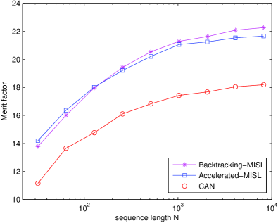
Figure 1: Merit factor (MF) versus sequence length. Each curve is averaged over 100 random trials.

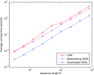
Figure 2: Average running time versus sequence length. Each curve is averaged over 100 random trials.

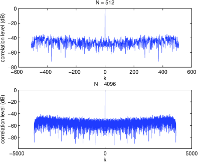
Figure 3: Correlation level of two sequences of length $N=512$ and $N=4096$, generated by the accelerated-MISL algorithm.

Next, we perform an experiment to show the different convergence properties of the proposed accelerated-MISL algorithm and the CAN algorithm. For both algorithms, we first initialize them with the same randomly generated sequence. Then we initialize CAN with the output sequence of accelerated-MISL and initialize accelerated-MISL with the output sequence of CAN, and run the two algorithms again. The evolution curves of the ISL in two different random trails with $N=32$ are shown in Fig. 4(a) and 4(b). From the figures, we can see that when initialized with the output sequence of CAN, the accelerated-MISL can further decrease the ISL a little bit, which means the point CAN converges to is probably not a local minimum. While in contrast, when initialized with the output sequence of accelerated-MISL, CAN increases the ISL, which means the point accelerated-MISL converges to is probably a local optimal and also tells the fact that CAN does not share the monotonicity of MISL. In addition, we can also see that when initialized with different sequences, CAN and accelerated-MISL may converge to different points. Thus, initializing the algorithms with good sequences, e.g. Frank sequence [12], Golomb sequence [13], can probably improve the performance of the algorithms.

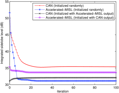
(a)

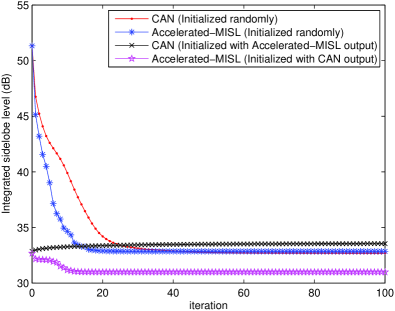
(b)

Figure 4: Evolution of the Integrated sidelobe level (ISL) in two different random trails with $N=32$.

Finally, we present an example of applying the accelerated-MISL algorithm to design unimodular sequences with impulse-like periodic autocorrelations. Recall that in the periodic case, unimodular sequences with exact impulsive autocorrelation (i.e., zero ISL) exist for any length $N$. The periodic correlation levels of two generated sequences of length $N=256$ and $N=1024$ are shown in Fig. 5, where the periodic correlation level is defined as in the aperiodic case.

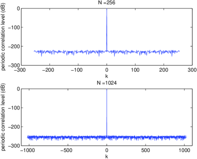
Figure 5: Periodic correlation level of two sequences of length $N=256$ and $N=1024$.

From Fig. 5, we can see that the periodic correlation levels of the two sequences are indeed very close to zero (lower than -200dB) at lags $k\neq 0$.

VI-B Spectral-MISL

In this subsection, we consider the design of a sequence of length $N=1000$ with low autocorrelation sidelobes and at the same time with low spectral power in the frequency bands $[\frac{\pi}{4},\frac{\pi}{2})\cup[\frac{3\pi}{4},\pi)\cup[\frac{3\pi}{2},\frac{7\pi}{4})$. To achieve this, we set the index set in spectral-MISL as $\Omega=\{250,\ldots,499\}\cup\{750,\ldots,999\}\cup\{1500,\ldots,1749\}$ accordingly and tune the parameter $\lambda$ to adjust the tradeoff between minimizing the correlation level and restricting the power in the pre-specified frequency bands. Fig. 6 shows the spectral power of the output sequence generated by spectral-MISL when initialized with a random sequence and with parameter $\lambda=10^{4}$. The correlation level of the same output sequence is shown in Fig. 7. We can see from the figures that the power in the pre-specified frequency bands has been suppressed and the correlation sidelobes are still relatively low.

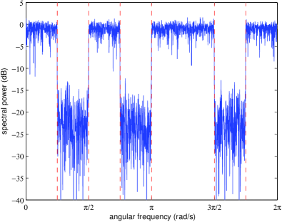
Figure 6: Spectral power of the designed sequence of length $N=1000,$ generated by spectral-MISL with $\lambda=10^{4}$.

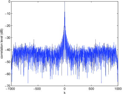
Figure 7: Correlation level of the designed sequence of length $N=1000,$ generated by spectral-MISL with $\lambda=10^{4}$.

VII Conclusion

We have presented an efficient algorithm named MISL for the minimization of the ISL metric of unimodular sequences. The MISL algorithm is derived based on the general majorization-minimization scheme and the convergence to a stationary point is guaranteed. Acceleration schemes that can be used to speed up MISL have also been considered. Numerical results show that in the case of aperiodic autocorrelations the proposed MISL algorithm can generate sequences with larger merit factor than the state-of-the-art method and in the case of periodic autocorrelations, MISL can produce sequences with virtually zero autocorrelation sidelobes. A MISL-like algorithm, i.e., spectral-MISL, has also been developed to minimize the ISL metric when there are additional spectral constraints. Numerical experiments show that the spectral-MISL algorithm can be used to design sequences with spectral power suppressed in arbitrary frequency bands and at the same time with low autocorrelation sidelobes. All the proposed algorithms can be implemented by means of the FFT and thus are computationally very efficient in practice.

-A Proof of $\lambda_{{\rm max}}(\mathbf{\Phi})=2N^{2}$

Proof:

We first recall that

$$\mathbf{\Phi}=\sum_{p=1}^{2N}{\rm vec}(\mathbf{A}_{p}){\rm vec}(\mathbf{A}_{p})^{H},$$ (65)

where $\mathbf{A}_{p}=\mathbf{a}_{p}\mathbf{a}_{p}^{H}$, $\mathbf{a}_{p}=[1,e^{j\omega_{p}},\cdots,e^{j\omega_{p}(N-1)}]^{T}$ and $\omega_{p}=\frac{2\pi}{2N}(p-1),\>p=1,\cdots,2N.$ The $(m,n)$-th element of matrix $\mathbf{A}_{p}$ is given by $\left[\mathbf{A}_{p}\right]_{m,n}=e^{j\omega_{p}(m-n)},\,m=1,\ldots,N,\,n=1,\ldots,N,$ which is also the $\left(m+(n-1)N\right)$-th element of ${\rm vec}(\mathbf{A}_{p})$. Then the $\left(m_{1}+(n_{1}-1)N,m_{2}+(n_{2}-1)N\right)$-th element of the matrix ${\rm vec}(\mathbf{A}_{p}){\rm vec}(\mathbf{A}_{p})^{H}$ is given by $\left[{\rm vec}(\mathbf{A}_{p}){\rm vec}(\mathbf{A}_{p})^{H}\right]_{m_{1}+(n_{1}-1)N,m_{2}+(n_{2}-1)N}=e^{j\omega_{p}(m_{1}-n_{1}-m_{2}+n_{2})},\,m_{1}=1,\ldots,N,\,n_{1}=1,\ldots,N,\,m_{2}=1,\ldots,N,\,n_{2}=1,\ldots,N.$ Then it is easy to see that

$$\left[\Phi\right]_{m_{1}+(n_{1}-1)N,m_{2}+(n_{2}-1)N} =\sum_{p=1}^{2N}e^{j\omega_{p}(m_{1}-n_{1}-m_{2}+n_{2})}$$

$$=\begin{cases}2N,&m_{1}-m_{2}=n_{1}-n_{2}\\ 0,&{\rm otherwise}.\end{cases}$$ (66)

We can see that $\mathbf{\Phi}$ is a real matrix.

To prove $\lambda_{{\rm max}}(\mathbf{\Phi})=2N^{2},$ we will show that $\mathbf{x}^{T}\left(2N^{2}\mathbf{I}-\mathbf{\Phi}\right)\mathbf{x}\geq 0,\,\forall\mathbf{x}\in\mathbf{R}^{N^{2}}$ and the equality is achievable for some $\mathbf{x}\neq\mathbf{0}.$ Let us define $\mathcal{I}_{0}=\{1,N+2,\ldots,N^{2}-N-1,N^{2}\},$ $\mathcal{I}_{-1}=\{2,N+3,\ldots,(N-1)N\},$ $\mathcal{I}_{1}=\{N+1,2N+2,\ldots,N^{2}-1\},\ldots,\mathcal{I}_{1-N}=\{N\}$ and $\mathcal{I}_{N-1}=\{N^{2}-N+1\}.$ It can be shown that

$$\mathbf{x}^{T}\left(2N^{2}\mathbf{I}-\mathbf{\Phi}\right)\mathbf{x}$$ (67)

$$= 2N\left(\sum_{k=1-N}^{N-1}\sum_{i,j\in\mathcal{I}_{k},i\neq j}(x_{i}-x_{j})^{2}+\sum_{k=1-N}^{N-1}\sum_{i\in\mathcal{I}_{k}}\left|k\right|x_{i}^{2}\right).$$

From (67), it is easy to see that $\mathbf{x}^{T}\left(2N^{2}\mathbf{I}-\mathbf{\Phi}\right)\mathbf{x}\geq 0,\,\forall\mathbf{x}\in\mathbf{R}^{N^{2}}$ and the equality holds for all $\mathbf{x}\in\mathbf{R}^{N^{2}}$ with the following structure:

$$\begin{cases}x_{i}=x_{j},&i,j\in\mathcal{I}_{0}\\ x_{i}=0,&{\rm otherwise}.\end{cases}$$

The proof is complete. ∎

References

- [1] R. Turyn, “Sequences with small correlation,” Error correcting codes, pp. 195–228, 1968.
- [2] S. W. Golomb and G. Gong, Signal Design for Good Correlation: For Wireless Communication, Cryptography, and Radar. Cambridge University Press, 2005.
- [3] N. Levanon and E. Mozeson, Radar Signals. John Wiley & Sons, 2004.
- [4] H. He, J. Li, and P. Stoica, Waveform Design for Active Sensing Systems: A Computational Approach. Cambridge University Press, 2012.
- [5] M. Golay, “A class of finite binary sequences with alternate auto-correlation values equal to zero (corresp.),” IEEE Transactions on Information Theory, vol. 18, no. 3, pp. 449–450, May 1972.
- [6] R. Barker, “Group synchronizing of binary digital systems,” Communication theory, pp. 273–287, 1953.
- [7] M. J. Golay, “Sieves for low autocorrelation binary sequences,” IEEE Transactions on Information Theory, vol. 23, no. 1, pp. 43–51, 1977.
- [8] S. Mertens, “Exhaustive search for low-autocorrelation binary sequences,” Journal of Physics A: Mathematical and General, vol. 29, no. 18, pp. 473–481, 1996.
- [9] S. Kocabas and A. Atalar, “Binary sequences with low aperiodic autocorrelation for synchronization purposes,” IEEE Communications Letters, vol. 7, no. 1, pp. 36–38, Jan. 2003.
- [10] J. Jedwab, “A survey of the merit factor problem for binary sequences,” in Sequences and Their Applications-SETA 2004. Springer, 2005, pp. 30–55.
- [11] S. Wang, “Efficient heuristic method of search for binary sequences with good aperiodic autocorrelations,” Electronics Letters, vol. 44, no. 12, pp. 731–732, 2008.
- [12] R. L. Frank, “Polyphase codes with good nonperiodic correlation properties,” IEEE Transactions on Information Theory, vol. 9, no. 1, pp. 43–45, Jan. 1963.
- [13] N. Zhang and S. W. Golomb, “Polyphase sequence with low autocorrelations,” IEEE Transactions on Information Theory, vol. 39, no. 3, pp. 1085–1089, 1993.
- [14] P. Borwein and R. Ferguson, “Polyphase sequences with low autocorrelation,” IEEE Transactions on Information Theory, vol. 51, no. 4, pp. 1564–1567, 2005.
- [15] C. Nunn and G. Coxson, “Polyphase pulse compression codes with optimal peak and integrated sidelobes,” IEEE Transactions on Aerospace and Electronic Systems, vol. 45, no. 2, pp. 775–781, Apr. 2009.
- [16] A. De Maio, S. De Nicola, Y. Huang, Z.-Q. Luo, and S. Zhang, “Design of phase codes for radar performance optimization with a similarity constraint,” IEEE Transactions on Signal Processing, vol. 57, no. 2, pp. 610–621, Feb. 2009.
- [17] P. Stoica, H. He, and J. Li, “New algorithms for designing unimodular sequences with good correlation properties,” IEEE Transactions on Signal Processing, vol. 57, no. 4, pp. 1415–1425, 2009.
- [18] M. Soltanalian and P. Stoica, “Computational design of sequences with good correlation properties,” IEEE Transactions on Signal Processing, vol. 60, no. 5, pp. 2180–2193, May 2012.
- [19] P. Stoica, H. He, and J. Li, “On designing sequences with impulse-like periodic correlation,” IEEE Signal Processing Letters, vol. 16, no. 8, pp. 703–706, Aug. 2009.
- [20] H. He, P. Stoica, and J. Li, “Waveform design with stopband and correlation constraints for cognitive radar,” in 2nd International Workshop on Cognitive Information Processing (CIP), Elba Island, Italy, Jun. 2010, pp. 344–349.
- [21] D. R. Hunter and K. Lange, “A tutorial on MM algorithms,” The American Statistician, vol. 58, no. 1, pp. 30–37, 2004.
- [22] M. Razaviyayn, M. Hong, and Z.-Q. Luo, “A unified convergence analysis of block successive minimization methods for nonsmooth optimization,” SIAM Journal on Optimization, vol. 23, no. 2, pp. 1126–1153, 2013.
- [23] G. Scutari, F. Facchinei, P. Song, D. P. Palomar, and J.-S. Pang, “Decomposition by partial linearization: Parallel optimization of multi-agent systems,” IEEE Transactions on Signal Processing, vol. 62, no. 3, pp. 641–656, Feb. 2014.
- [24] D. P. Bertsekas, A. Nedić, and A. E. Ozdaglar, Convex Analysis and Optimization. Athena Scientific, 2003.
- [25] R. Varadhan and C. Roland, “Simple and globally convergent methods for accelerating the convergence of any EM algorithm,” Scandinavian Journal of Statistics, vol. 35, no. 2, pp. 335–353, 2008.
- [26] M. Raydan and B. F. Svaiter, “Relaxed steepest descent and Cauchy-Barzilai-Borwein method,” Computational Optimization and Applications, vol. 21, no. 2, pp. 155–167, 2002.
- [27] J. Barzilai and J. M. Borwein, “Two-point step size gradient methods,” IMA Journal of Numerical Analysis, vol. 8, no. 1, pp. 141–148, 1988.
- [28] S. Haykin, “Cognitive radar: a way of the future,” IEEE Signal Processing Magazine, vol. 23, no. 1, pp. 30–40, Jan. 2006.