Status of the Higgs Singlet Extension of the Standard Model after LHC Run 1
Abstract
We discuss the current status of theoretical and experimental constraints on the real Higgs singlet extension of the Standard Model. For the second neutral (non-standard) Higgs boson we consider the full mass range from to accessible at past and current collider experiments. We separately discuss three scenarios, namely, the case where the second Higgs boson is lighter than, approximately equal to, or heavier than the discovered Higgs state at around . We investigate the impact of constraints from perturbative unitarity, electroweak precision data with a special focus on higher order contributions to the boson mass, perturbativity of the couplings as well as vacuum stability. The latter two are tested up to a scale of using renormalization group equations. Direct collider constraints from Higgs signal rate measurements at the LHC and exclusion limits from Higgs searches at LEP, Tevatron and LHC are included via the public codes HiggsSignals and HiggsBounds, respectively. We identify the strongest constraints in the different regions of parameter space. We comment on the collider phenomenology of the remaining viable parameter space and the prospects for a future discovery or exclusion at the LHC.
I Introduction
The LHC discovery atlres ; cmsres of a Higgs boson in July 2012 has been a major breakthrough in modern particle physics. The first runs of the LHC at and are now completed and the main results from various experimental analyses of the Higgs boson properties have been presented at the 2014 summer conferences. So far, the discovered state is well compatible Aad:2013xqa ; Aad:2014eha ; Aad:2014eva ; Aad:2014xzb ; Khachatryan:2014ira ; Chatrchyan:2014vua ; Chatrchyan:2013mxa ; Chatrchyan:2013iaa with the interpretation in terms of the scalar boson of the Standard Model (SM) Higgs mechanism Higgs:1964ia ; Higgs:1964pj ; Englert:1964et ; Guralnik:1964eu ; Kibble:1967sv . A simple combination of the Higgs mass measurements performed by ATLAS Aad:2014aba and CMS CMS:2014ega yields a central value of
| (1) |
If the discovered particle is indeed the Higgs boson predicted by the SM, its mass constitutes the last unknown ingredient to this model, as all other properties of the electroweak sector then follow directly from theory. The current and future challenge for the theoretical and experimental community is to thoroughly investigate the Higgs boson’s properties in order to identify whether the SM Higgs sector is indeed complete, or instead, the structure of a more involved Higgs sector is realized. On the experimental side, this requires detailed and accurate measurements of its coupling strengths and structure at the LHC and ultimately at future experimental facilities for Higgs boson precision studies, such as the International Linear Collider (ILC) Asner:2013psa . A complementary and equally important strategy is to perform collider searches for additional Higgs bosons. Such a finding would provide clear evidence for a non-minimal Higgs sector. This road needs to be continued within the full mass range that is accessible to current and future experiments.
In this work, we consider the simplest extension of the SM Higgs sector, where an additional real singlet field is added, which is neutral under all quantum numbers of the SM gauge group Schabinger:2005ei ; Patt:2006fw and acquires a vacuum expectation value (VEV). This model has been widely studied in the literature Barger:2007im ; Bhattacharyya:2007pb ; Dawson:2009yx ; Bock:2010nz ; Fox:2011qc ; Englert:2011yb ; Englert:2011us ; Batell:2011pz ; Englert:2011aa ; Gupta:2011gd ; Dolan:2012ac ; Bertolini:2012gu ; Batell:2012mj ; Lopez-Val:2013yba ; Heinemeyer:2013tqa ; Chivukula:2013xka ; Englert:2013tya ; Cooper:2013kia ; Caillol:2013gqa ; Coimbra:2013qq ; Pruna:2013bma ; Dawson:2013bba ; Lopez-Val:2014jva ; Englert:2014aca ; Englert:2014ffa ; Chen:2014ask ; Karabacak:2014nca ; Profumo:2014opa . Here, we present a complete exploration of the model parameter space in the light of the latest experimental and theoretical constraints. We consider masses of the second (non-standard) Higgs boson in the whole mass range up to , thus extending and updating the findings of previous work Pruna:2013bma . This minimal setup can be interpreted as a limiting case for more generic BSM scenarios, e.g. models with additional gauge sectors Basso:2010jm or additional matter content Strassler:2006im ; Strassler:2006ri .
In our analysis, we study the implications of various constraints: We take into account bounds from perturbative unitarity and electroweak (EW) precision measurements, in particular focussing on higher order corrections to the boson mass Lopez-Val:2014jva . Furthermore, we study the impact of requiring perturbativity, vacuum stability and correct minimization of the model up to a high energy scale using renormalization group evolved couplings111The value of this high energy scale is chosen to be larger than the energy scale where the running SM Higgs quartic coupling turns negative. This will be made more precise in Section III.. We include the exclusion limits from Higgs searches at the LEP, Tevatron and LHC experiments via the public tool HiggsBounds Bechtle:2008jh ; Bechtle:2011sb ; Bechtle:2013gu ; Bechtle:2013wla , and use the program HiggsSignals Bechtle:2013xfa (cf. also Ref. Bechtle:2014ewa ) to test the compatibility of the model with the signal strength measurements of the discovered Higgs state.
We separate the discussion of the parameter space into three different mass regions: (i) the high mass region, , where the lighter Higgs boson is interpreted as the discovered Higgs state; (ii) the intermediate mass region, where both Higgs bosons and are located in the mass region and potentially contribute to the measured signal rates and (iii) the low mass region, , where the heavier Higgs boson is interpreted as the discovered Higgs state.
We find that the most severe constraints in the whole parameter space for the second Higgs mass are mostly given by limits from collider searches for a SM Higgs boson as well as by the LHC Higgs boson signal strength measurements. For limits from higher order contributions to the boson mass prevail, followed by the requirement of perturbativity of the couplings which is tested via renormalization group equation (RGE) evolution. For the remaining viable parameter space we present predictions for signal cross sections of the yet undiscovered second Higgs boson for the LHC at center-of-mass (CM) energies of and , discussing both the SM Higgs decay signatures and the novel Higgs-to-Higgs decay mode . We furthermore present our results in terms of a global suppression factor for SM-like channels as well as the total width of the second Higgs boson, and show regions which are allowed in the plane.
The paper is organized as follows: In Section II we briefly review the model and the chosen parametrization. In Section III we elaborate upon the various theoretical and experimental constraints and discuss their impact on the model parameter space. In Section IV a scan of the full model parameter space is presented, in which all relevant constraints are combined. This is followed by a discussion of the collider phenomenology of the viable parameter space. We summarize and conclude in Section V.
II The model
II.1 Potential and couplings
The real Higgs singlet extension of the SM is described in detail in Refs. Schabinger:2005ei ; Patt:2006fw ; Bowen:2007ia ; Pruna:2013bma . Here, we only briefly review the theoretical setup as well as the main features relevant to the work presented here.
We consider the extension of the SM electroweak sector containing a complex doublet, in the following denoted by , by an additional real scalar which is a singlet under all SM gauge groups. The most generic renormalizable Lagrangian is then given by
| (2) |
with the scalar potential
| (8) | |||||
| (9) |
Here, we implicitly impose a symmetry which forbids all linear or cubic terms of the singlet field in the potential. The scalar potential is bounded from below if the following conditions are fulfilled:
| (10) | |||||
| (11) |
cf. Appendix A. If the first condition, Eq. (10), is fulfilled, the extremum is a local minimum. The second condition, Eq. (11), guarantees that the potential is bounded from below for large field values. We assume that both Higgs fields and have a non-zero vacuum expectation value (VEV), denoted by and , respectively. In the unitary gauge, the Higgs fields are given by
| (12) |
Expansion around the minimum leads to the squared mass matrix
| (15) |
with the mass eigenvalues
| (16) | ||||
| (17) |
where and are the scalar fields with masses and respectively, and by convention. Note that follows from Eq. (10) and we assume Eqs. (10) and (11) to be fulfilled in all following definitions. The gauge and mass eigenstates are related via the mixing matrix
| (18) |
where the mixing angle is given by
| (19) | ||||
| (20) |
It follows from Eq. (18) that the light (heavy) Higgs boson couplings to SM particles are suppressed by .
Using Eqs. (16), (17) and (19), we can express the couplings in terms of the mixing angle , the Higgs VEVs and and the two Higgs boson masses, and :
| (21) |
If kinematically allowed, the additional decay channel is present. Its partial decay width is given by Schabinger:2005ei ; Bowen:2007ia
| (22) |
where the coupling strength of the decay reads
| (23) |
We therefore obtain as branching ratios for the heavy Higgs mass eigenstate
| (24) |
where denotes the partial decay width of the SM Higgs boson and represents any SM Higgs decay mode. The total width is given by
where denotes the total width of the SM Higgs boson with mass . The suppression by directly follows from the suppression of all SM–like couplings, cf. Eq. (18). For , we recover the SM Higgs boson branching ratios.
For collider phenomenology, two features are important:
-
•
the suppression of the production cross section of the two Higgs states induced by the mixing, which is given by for the heavy (light) Higgs, respectively;
-
•
the suppression of the Higgs decay modes to SM particles, which is realized if the competing decay mode is kinematically accessible.
For the high mass (low mass) scenario, i.e. the case where the light (heavy) Higgs boson is identified with the discovered Higgs state at , corresponds to the complete decoupling of the second Higgs boson and therefore the SM-like scenario.
II.2 Model parameters
At the Lagrangian level, the model has five free parameters,
| (25) |
while the values of the additional parameters are fixed by the minimization conditions to the values
| (26) | ||||
| (27) |
cf. Appendix A. In this work, we choose to parametrize the model in terms of the independent physical quantities
| (28) |
The couplings and can then be expressed via Eq. (II.1). The vacuum expectation value of the Higgs doublet is given by the SM value . Unless otherwise stated, we fix one of the Higgs masses to be , hence interpreting the Higgs boson as the discovered Higgs state at the LHC. In this case, we are left with only three independent parameters, , where the latter enters the collider phenomenology only via the additional decay channel222In fact, all Higgs self-couplings depend on . However, in the factorized leading-order description of production and decay followed here, and as long as no experimental data exists which constrains the Higgs boson self-couplings, only the coupling needs to be considered. .
III Theoretical and experimental constraints
We now discuss the various theoretical and experimental constraints on the singlet extension model. In our analysis, we impose the following constraints:
-
(1.)
limits from perturbative unitarity,
-
(2.)
limits from from EW precision data in form of the parameters Altarelli:1990zd ; Peskin:1990zt ; Peskin:1991sw ; Maksymyk:1993zm as well as the singlet–induced NLO corrections to the boson mass as presented in Ref. Lopez-Val:2014jva ,
- (3.)
-
(4.)
limits from perturbativity of the couplings as well as vacuum stability up to a certain scale , where we chose as benchmark point (these constraints will only be applied in the high mass region, see Section III.3 for further discussion),
-
(5.)
upper cross section limits at from null results in Higgs searches at the LEP, Tevatron and LHC experiments,
-
(6.)
consistency with the Higgs boson signal rates measured at the LHC experiments.
The constraints (1.) – (4.) have already been discussed extensively in a previous publication Pruna:2013bma , where the scan was however restricted to the case that . In the following, we will therefore briefly recall the definition of the theoretically motivated bounds and comment on their importance in the whole mass range .
III.1 Perturbative unitarity
Tree-level perturbative unitarity Lee:1977eg ; Luscher:1988gc puts a constraint on the Higgs masses via a relation on the partial wave amplitudes of all possible scattering processes:
| (29) |
where the partial wave amplitude poses the strongest constraint. Following Ref. Pruna:2013bma , we consider all processes , with , and impose the condition of Eq. (29) to the eigenvalues of the diagonalized scattering matrix. Note that the unitarity constraint based on the consideration of scattering alone, leading to (as e.g. in Ref. Englert:2011yb ), is much loosened when all scattering channels are taken into account Bowen:2007ia ; Basso:2010jt .
In general, perturbative unitarity poses an upper limit on . In the decoupling case, which corresponds to for the light (heavy) Higgs being SM-like, it is given by Pruna:2013bma
| (30) |
where and refer to the purely singlet Higgs state and its respective mass.
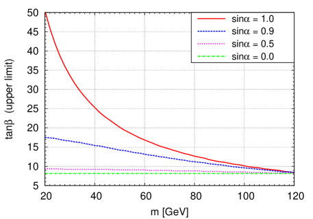
While in the high mass scenario this bound is always superseded by bounds from perturbativity of the couplings, cf. Section III.3, in the low mass scenario this poses the strongest theoretical bound on . We exemplarily show the upper limits on derived from perturbative unitarity in Fig. 1 for the low mass range for the four values of . The bounds on are strongest for small values of . However, values too far from the decoupling case are highly constrained by Higgs searches at LEP as well as by the LHC signal strength measurements of the heavier Higgs at , cf. Sections III.5 and III.6 for more details.
III.2 Perturbativity of the couplings
For perturbativity of the couplings, we require that
| (31) |
At the electroweak scale, these bounds do not pose additional constraints on the parameter space after limits from perturbative unitarity have been taken into account.
III.3 Renormalization group equation evolution of the couplings
While perturbativity as well as vacuum stability and the existence of a local minimum at the electroweak scale are necessary ingredients for the validity of a parameter point, it is instructive to investigate up to which energy scale these requirements remain valid. In particular, we study whether the potential is bounded from below and features a local minimum at energy scales above the electroweak scale. In order to achieve this, we promote the requirements of Eqs. (10), (11), and (31) to be valid at an arbitrary scale , where are evolved according to the one-loop renormalization group equations (RGEs) (see e.g. Ref. Lerner:2009xg )
| (32) | ||||
| (33) | ||||
| (34) |
Here we introduced as a dimensionless running parameter. The initial conditions at the electroweak scale require that are given by Eqn. (II.1). The top Yukawa coupling as well as the SM gauge couplings evolve according to the one-loop SM RGEs, cf. Appendix B. For the decoupling case as well as to cross-check the implementation of the running of the gauge couplings we reproduced the results of Ref. Degrassi:2012ry .
As in Ref. Pruna:2013bma , we require all RGE-dependent constraints to be valid at a scale which is slightly higher than the breakdown scale of the SM, such that the singlet extension of the SM improves the stability of the electroweak vacuum. The SM breakdown scale is defined as the scale where the potential becomes unbounded from below in the decoupled, SM-like scenario. With the input values of and , a top mass of as well as a top-Yukawa coupling and strong coupling constant , we obtain as a SM breakdown scale333As has been discussed in e.g. Ref. Degrassi:2012ry , the scale where in the decoupling case strongly depends on the initial input parameters. However, as we are only interested in the difference of the running in the case of a non-decoupled singlet component with respect to the Standard Model, we do not need to determine this scale to the utmost precision. For a more thorough discussion of the behavior of the RGE-resulting constraints in case of varying input parameters, see e.g. Ref. Pruna:2013bma .
We therefore chose as a slightly higher test scale the value . Naturally, we only apply this test to points in the parameter space which have passed constraints from perturbative unitarity as well as perturbativity of the couplings at the electroweak scale. Changing the scale to higher (lower) values leads to more (less) constrained regions in the models parameter space Pruna:2013bma .
In the high mass scenario we see the behavior studied in Ref. Pruna:2013bma for Higgs masses continuing to the lower mass ranges. The strongest constraints that impact different parts of the parameter space are displayed in Fig. 2 for a heavy Higgs mass of (taken from Ref. Pruna:2013bma ). Two main features can be observed:
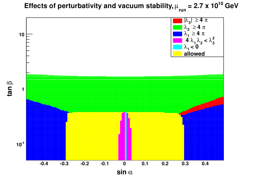
First, the upper value of for fixed Higgs masses is determined by requiring perturbativity of as well as perturbative unitarity, cf. Section III.1. Second, the allowed range of the mixing angle is determined by perturbativity of the couplings as well as the requirement of vacuum stability, especially when these are required at renormalization scales , which are significantly larger than the electroweak scale. Small mixings are excluded by the requirements of vacuum stability444For the requirement of vacuum stability, we found that in some cases the coupling strengths vary very mildly over large variations of the RGE running scale. In these regions the inclusion of higher order corrections in the spirit of Ref. Degrassi:2012ry seems indispensable. Therefore, all lower limits on the mixing angle originating from RGE constraints need to be viewed in this perspective. In fact, such higher order contributions to the scalar-extended RGEs have recently been presented in Ref. Costa:2014qga . However, the authors did not specifically investigate the higher order effects on parameter points which exhibit small variations over large energy scales at NLO. as well as minimization of the scalar potential. This corresponds to the fact that we enter an unstable vacuum for for .
In summary, the constraints from RGE evolution of the couplings pose the strongest bounds on the minimally allowed value and the maximal value of in the high mass scenario. Note that, for lower , the parameter space is less constrained, as will be discussed in Section IV.1.
In the low mass scenario, i.e. where the heavier Higgs state is considered to be the discovered Higgs boson, none of the points in our scan fulfilled vacuum stability above the electroweak scale. This is due to the fact that for a relatively low , the value of at the electroweak scale is quite small, cf. Eq. (II.1). In the non-decoupled case, , then receives negative contributions in the RG evolution towards higher scales, leading to already at relatively low scales , corresponding to the breakdown of the electroweak vacuum. Hence, in the low mass scenario, the theory breaks down even earlier than in the SM case. In the analysis presented here, we will therefore refrain from taking limits from RGE running into account in the low mass scenario. Then, the theoretically maximally allowed value of is determined from perturbative unitarity and rises to quite large values, where we obtain , depending on the value of the light Higgs mass .
Further constraints on in the low mass scenario stem from the Higgs signal rate observables through the potential decay , as will be discussed in Section III.6.
III.4 The boson mass and electroweak oblique parameters , ,
Recently, the one–loop corrections to the boson mass, , for this model have been calculated in Ref. Lopez-Val:2014jva . In that analysis, is required to agree within with the experimental value Alcaraz:2006mx ; Aaltonen:2012bp ; D0:2013jba , leading to an allowed range for the purely singlet-induced corrections of . Theoretical uncertainties due to contributions at even higher orders have been estimated to be . The one-loop corrections are independent555In the electroweak gauge sector, only enters at the 2–loop level when the Higgs mass sector is renormalized in the on–shell scheme. of and give rise to additional constraints on , which in the high mass scenario turn out to be much more stringent Lopez-Val:2014jva than the constraints obtained from the oblique parameters , and Altarelli:1990zd ; Peskin:1990zt ; Peskin:1991sw ; Maksymyk:1993zm .
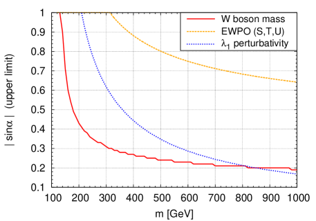
Figure 3 shows the maximally allowed mixing angle obtained from the constraint as a function of the heavy Higgs mass in the high mass scenario. For comparison, we also included the limit stemming from the electroweak oblique parameters , , and (see below), as well as from requiring perturbativity of , evaluated at . We see that for constraints from yield the strongest constraint. The oblique parameters , and do not pose additional limits on the allowed parameter space.
In the low mass region, as discussed in Ref. Lopez-Val:2014jva , the NLO contributions within the Higgs singlet extension model even tend to decrease the current discrepancy between the theoretical value in the SM Awramik:2003rn and the experimental measurement Alcaraz:2006mx ; Aaltonen:2012bp ; D0:2013jba . However, substantial reduction of the discrepancy only occurs if the light Higgs has a sizable doublet component. Hence, this possibility is strongly constrained by exclusion limits from LEP and/or LHC Higgs searches (depending on the light Higgs mass) as well as by the LHC Higgs signal rate measurements.
In the low mass region the electroweak oblique parameters pose non-negligible constraints, as will be shown in Section IV.2. However, these constraints are again superseded once the Higgs signal strength as well as direct search limits from LEP are taken into account, cf. Section III.5 and III.6 respectively.
In our analysis we test the constraints from the electroweak oblique parameters , and by evaluating
| (35) |
with , where the observed parameters are given by Baak:2014ora
| (36) |
and the unhatted quantities denote the model predictions Lopez-Val:2014jva .666The exact one–loop quantities from Ref. Lopez-Val:2014jva render qualitatively the same constraints as the values used in Ref. Pruna:2013bma , which were obtained from rescaled SM expressions Hagiwara:1994pw . The covariance matrix reads Baak:2014ora
| (40) |
We then require , corresponding to a maximal deviation given the three degrees of freedom.
III.5 Exclusion limits from Higgs searches at LEP and LHC
Null results from Higgs searches at collider experiments limit the signal strength of the second, non SM-like Higgs boson. Recall that its signal strength is given by the SM Higgs signal rate scaled by in the low mass region and, in the absence of Higgs-to-Higgs decays, in the high mass region. Thus, the exclusion limits can easily be translated into lower or upper limits on the mixing angle , respectively.777Here we neglect the possible influence of interference effects in the production of the light and heavy Higgs boson and its successive decay. Recent studies Hagiwara:2005wg ; Uhlemann:2008pm ; Kalinowski:2008fk ; Goria:2011wa ; Wiesler:2012rkl ; Kauer:2012hd ; Englert:2014aca ; Logan:2014ppa ; Maina:2015ela have shown that interference and finite width effect can lead to sizable deviations in the invariant mass spectra of prominent LHC search channels such as in the high mass region and thus should be taken into account in accurate experimental studies of the singlet extended SM at the LHC. However, the inclusion of these effects is beyond the scope of the work presented here.
We employ HiggsBounds-4.2.0 Bechtle:2008jh ; Bechtle:2011sb ; Bechtle:2013gu ; Bechtle:2013wla to derive the exclusion limits from collider searches. The exclusion limits from the LHC experiments888HiggsBounds also contains limits from the Tevatron experiments. In the singlet extended SM, however, these limits are entirely superseded by LHC results. are usually given at the . For most of the LEP results we employ the extension Bechtle:2013wla of the HiggsBounds package.999The LEP information is available for Higgs masses . For lower masses, we take the conventional output from HiggsBounds. The obtained value will later be added to the contribution from the Higgs signal rates, cf. Section III.6, to construct a global likelihood.
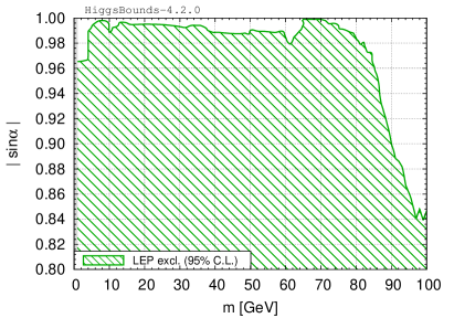
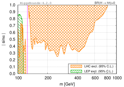
The C.L. excluded regions of derived with HiggsBounds are shown in Fig. 4 as a function of the second Higgs mass, assuming a vanishing decay width of the Higgs-to-Higgs decay mode . Since all Higgs boson production modes are reduced with respect to their SM prediction by a universal factor, limits from LHC Higgs search analyses for a SM Higgs boson can be applied straight-forwardly Bechtle:2013wla . In particular, the exclusion limits obtained from combinations of SM Higgs boson searches with various final states are highly sensitive. However, so far, such combinations have only been presented by ATLAS and CMS for the full dataset Chatrchyan:2012tx ; Aad:2012an and for a subset of the data CMS:aya . The strongest exclusions are therefore obtained mostly from the single search analyses of the full dataset, in particular from the channel ATLAS:2013nma ; Chatrchyan:2012dg ; CMS:xwa in the mass region and for , as well as from the channel ATLAS:2013wla ; Chatrchyan:2013iaa ; CMS:bxa in the mass region due to the irreducible background in the analyses. For Higgs masses the only LHC exclusion limits currently available are from the ATLAS search for scalar diphoton resonances Aad:2014ioa . However, these constraints are weaker than the LEP limits from the channel Schael:2006cr , as can be seen in Fig. 4(b). In the remaining mass regions with the CMS limit CMS:aya from the combination of SM Higgs analyses yields the strongest constraint. For very low Higgs masses, , the LEP constraints come from Higgs pair production processes, Schael:2006cr , as well as from the decay-mode independent analysis of by OPAL Abbiendi:2002qp . The latter analysis provides limits for Higgs masses as low as .
In the presence of Higgs-to-Higgs decays, , additional constraints arise. In case of very low masses, , these stem from the CMS search in the channel CMS:2013lea , and for large masses, , from the CMS search for with multileptons and photons in the final state CMS:2013eua . These limits will be discussed separately in Section IV. Note that the limit from SM Higgs boson searches in the mass range , as presented in Fig. 4(b), will diminish in case of non-vanishing due to a suppression of the SM Higgs decay modes. We find in the full scan (see Section IV) that, in general, can be as large as in this model. Neglecting the correlation between and for a moment, such large branching fractions could lead to a reduction of the upper limit on obtained from SM Higgs searches by a factor of . However, once all other constraints (in particular from the NLO calculation of ) are taken into account, only values of up to are found, see Section IV.1, Fig. 11(b). Moreover, in the mass region where the largest values of appear, the constraint on is typically stronger than the constraints from SM Higgs searches, even if is assumed in the latter. Therefore, given the present Higgs search exclusion limits, the signal rate reduction currently does not have a visible impact on the viable parameter space101010Note, however, that this may change in future with significantly improved exclusion limits from SM Higgs searches..
III.6 Higgs boson signal rates measured at the LHC
The compatibility of the predicted signal rates for the Higgs state at with the latest measurements from ATLAS Aad:2014eha ; Aad:2014eva ; ATLAS-WW-Note ; ATLAS-tautau-Note ; Aad:2014xzb and CMS Khachatryan:2014ira ; Chatrchyan:2013mxa ; Chatrchyan:2013iaa ; Chatrchyan:2014vua is evaluated with HiggsSignals-1.3.0 by means of a statistical measure. The implemented observables are listed in Tab. 1. In the following we denote this value by , which also includes the contribution from the Higgs mass observables evaluated within HiggsSignals. The latter, however, only yields non-trivial constraints on the parameter space if the fit allows a varying Higgs mass in the vicinity of . In the low mass scenario, where one of the Higgs bosons is within the kinematical range of the LEP experiment, the value obtained from the HiggsBounds LEP extension, denoted as , is added to the HiggsSignals to construct the global likelihood
| (41) |
The and confidence level () parameter regions of the model are approximated by the difference to the minimal value found at the best-fit point, , taking on values of and in the case of a -dimensional projected parameter space, respectively.
| experiment | channel | obs. signal rate | obs. mass [] |
|---|---|---|---|
| ATLAS | ATLAS-WW-Note | – | |
| ATLAS | Aad:2014eva | ||
| ATLAS | Aad:2014eha | ||
| ATLAS | ATLAS-tautau-Note | – | |
| ATLAS | Aad:2014xzb | – | |
| CMS | Chatrchyan:2013iaa | – | |
| CMS | Chatrchyan:2013mxa | ||
| CMS | Khachatryan:2014ira | ||
| CMS | Chatrchyan:2014vua | – | |
| CMS | Chatrchyan:2014vua | – |
When both Higgs masses are fixed, the fit depends on two free parameters, namely and . The latter can only influence the signal rates of the Higgs boson if the additional decay mode is accessible. The branching fraction then leads to a decrease of all other decay modes and hence to a reduction of the predictions for the measured signal rates, cf. Eq. (II.1). The sensitivity to via the signal rate measurements is thus only given if the heavier Higgs state is interpreted as the discovered particle, (low mass region), and the second Higgs state is sufficiently light, . If the decay is not kinematically accessible, or in the case where the light Higgs is considered as the discovered Higgs state at , there are no relevant experimental constraints on .
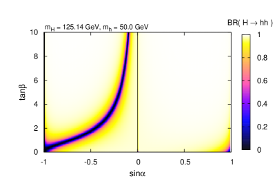
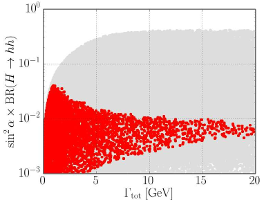
In the low mass region, the Higgs signal rate measurements constrain the modulus of the mixing angle to be close to , such that the heavy Higgs boson has nearly the same coupling strengths as the SM Higgs boson. Moreover, in order to obtain sizable predictions for the measured signal rates, the branching ratio must not be too large. We illustrate its dependence on in Fig. 5, where we exemplarily show the branching ratio in the (, ) plane for fixed Higgs boson masses of and . As can be seen in Fig. 5(a), the decay is dominant over large regions of the parameter space, with the exception of three distinct cases: The branching ratio exactly vanishes in the case that
| (42) |
In the first case (i) all couplings of the heavy Higgs boson to SM particles vanish completely, thus this case is highly excluded by observations. The second case (ii) corresponds to the complete decoupling of the lighter Higgs boson, such that the heavier Higgs is identical to the SM Higgs boson. In the third and more interesting case (iii) the branching fraction can be expanded in powers of :
where is the total width in the SM for a Higgs boson at mass .
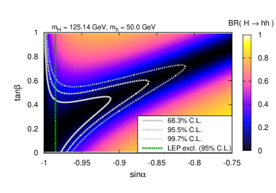
In Fig. 5(b) we show a zoom of the (, ) plane, focussing on the low- valley and values close to . We furthermore indicate the parameter regions which are allowed at the , and level by the Higgs signal rate measurements by the gray contour lines. The maximally values of allowed by the Higgs signal rate measurements at are found for very close to and large values, i.e. in the vicinity of case (ii) discussed above. In the given example with , the exclusion from LEP searches, as discussed in Section III.5 (cf. Fig. 4(a)), imposes and is indicated in Fig. 5(b) by the green, dashed line.
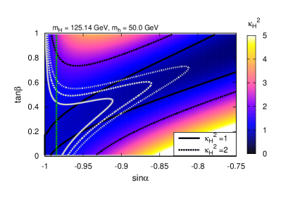
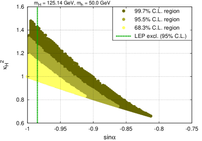
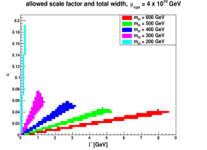
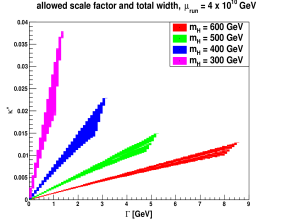
Finally, we plot the total width scaling factor, defined by , in the (, ) plane in Fig. 6(a). We furthermore plot for the parameter regions favored by the Higgs signal rates in Fig. 6(b). The largest values of allowed by both the signal rates and the LEP constraints at are obtained for close to . In the example of discussed here, the total width is increased by up to around with respect to the SM. This maximal value of total width enhancement is independent of the light Higgs mass (assuming that the channel is kinematically accessible).
We now want to draw the attention to the intermediate mass range, where both mass eigenstates can contribute to the signal strength measurements at the LHC. If the masses of the two Higgs bosons are well separated, the signal yields measured in the LHC Higgs analyses can be assumed to be solely due to the one Higgs boson lying in the vicinity of the signal, . However, in analyses with a poor mass resolution, as is typically the case in search analyses for the decay modes , and , the signal contamination from the second Higgs boson needs to be taken into account if its mass is not too far away from . While a proper treatment of this case can only be done by the experimental analyses, HiggsSignals employs a Higgs boson assignment procedure to approximately account for this situation Bechtle:2013xfa . Based on the experimental mass resolution of the analysis and the difference between the predicted mass and the mass position where the measurement has been performed, HiggsSignals decides whether the signal rates of multiple Higgs states need to be combined. Hence, superpositions of the two Higgs signal rates considered here are possible if the second Higgs mass lies within .
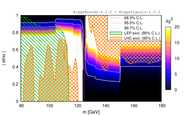
In Fig. 7 we show the HiggsSignals value obtained from the signal rate observables as a function of the second Higgs boson mass and the mixing angle . The mass of the other Higgs boson is fixed at . The scan range for extends over both the low mass and high mass region. Since the Higgs boson at needs sufficiently large signal rates to accommodate for the observed SM-like Higgs signal strength, small (large) values of are favored in the high (low) mass region, such that the second Higgs boson is rather decoupled. We furthermore show the parameter space excluded at by LEP and LHC searches, as previously discussed in Section III.5 in Fig. 4.
In the case of nearly mass degenerate Higgs bosons, , the sensitivity on the mixing angle significantly decreases, as the signal rates of the two Higgs states are always superimposed. There remains a slight dependence of the total signal rate on the Higgs masses, though, since the production cross sections and branching ratios are mass dependent. Moreover, depending on the actual mass splitting and mixing angle, potential effects may possibly be seen in the invariant mass distributions of the high-resolution LHC channels Khachatryan:2014ira and , at a future linear collider like the ILC Asner:2013psa ; Dawson:2013bba or eventually a muon collider Alexahin:2013ojp ; Dawson:2013bba . However, the sensitivity on completely vanishes in the case of exact mass degeneracy, , such that the singlet extended SM becomes indistinguishable from the SM.
The weak dependence on outside of the mass degenerate region, i.e. for and , is caused by the superposition of the signal rates of both Higgs bosons in some of the and channels, as discussed above. These structures depend on the details of the implementation within HiggsSignals, in particular on the assumed experimental resolution for each analysis. For Higgs masses below and beyond around the limit from the signal rates is independent111111This statement is only true if the Higgs state at does not decay to the lighter Higgs. As discussed above, at low light Higgs masses , the branching ratio can reduce the signal rates of the heavy Higgs decaying to SM particles. of .
We see that for Higgs masses in the range between and , the constraints from the Higgs signal rates are more restrictive than the exclusion limits from Higgs searches at LEP and LHC. For lower Higgs masses, , the LEP limits (cf. Fig. 4(a)) generally yield stronger constraints on the parameter space. For higher Higgs masses, , the direct LHC limits (cf. Fig. 4(b)) are slightly stronger than the constraints from the signal rates, however, this picture reverses again for Higgs masses beyond , where direct heavy Higgs searches become less sensitive.
IV Results of the Full Parameter Scan
In this section we investigate the interplay of all theoretical and experimental constraints discussed in the previous section on the real singlet extended SM parameter space, specified by
We separate the discussion into the high mass, the low mass and the intermediate (or degenerate) mass region of the parameter space. In the high and low mass region, we keep one of the Higgs masses fixed at and vary the other, while in the intermediate mass region we treat both Higgs masses as scan parameters. In the following we first present results for fixed mass in order to facilitate the understanding of the respective parameter space in dependence of . These discussions will then be extended by a more general scan, where all parameters are allowed to vary simultaneously. For each of these scans, we generate around points. We close the discussion of each mass region by commenting on the relevant collider phenomenology.
IV.1 High mass region
In this section, we explore the parameter space of the high mass region, . In general, for masses , our results agree with those presented in Ref. Pruna:2013bma . However, we obtain stronger bounds on the maximally allowed value of due to the constraints from the NLO calculation of Lopez-Val:2014jva , which has not been available for the previous analysis Pruna:2013bma . As has been discussed in Section III.4, Fig. 3, the constraints from are much more stringent than those obtained from the oblique parameters , , and in the high mass region.

| source upper limit | |||
|---|---|---|---|
| perturbativity | |||
| perturbativity | |||
| at NLO | |||
| at NLO | |||
| at NLO | |||
| at NLO | |||
| at NLO | |||
| at NLO | |||
| at NLO | |||
| signal rates | |||
| signal rates | |||
| signal rates |
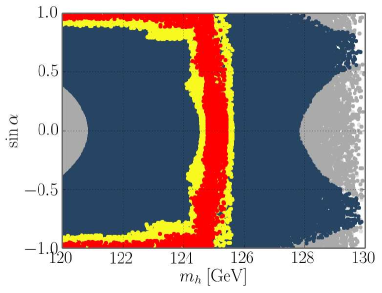
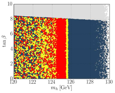
We compile all previously discussed constraints on the maximal mixing angle in Fig. 8. Furthermore, the (one-dimensional) allowed regions in and are given in Tab. 2 for fixed values of .121212Note, that the upper limit on from the Higgs signal rates is based on a two-dimensional profile (for floating ) in Fig. 8, whereas in Tab. 2 the one-dimensional profile (for fixed ) is used. This leads to small differences in the obtained limit. Here, the allowed range of is evaluated for fixed and we explicitly specify the relevant constraint that provides in the upper limit on . We find the following generic features: For Higgs masses , the boson mass NLO calculation provides the upper limit on , at lower masses the LHC constraints at from direct Higgs searches and the signal rate measurements are most relevant. The purely theory-based limits from perturbativity of only become important for . Furthermore, in the whole mass range, the minimal value of and the maximal value of are determined by vacuum stability and perturbativity of the couplings.
The corresponding (two-dimensional) allowed regions in the () plane for fixed Higgs masses are shown in Fig. 9. Their shapes are largely dictated by the perturbativity and vacuum stability requirements of the RGE evolved couplings, thus basically resembling the features observed before in Fig. 2 for . Here, however, the maximally allowed values for the mixing angle stem now from the NLO calculation of or, at rather low masses , from the Higgs signal rates and/or exclusion limits. In all cases, the upper limit on stems from the perturbativity requirement of RGE evolved couplings. For the degenerate case, , we a priori find no upper or lower limit on the mixing angle. In the degenerate case we do not take limits from RGE running into account, hence the only constraint stems from perturbative unitarity which renders an upper limit on .
We now extend the discussion and treat as a free model parameter. The results are presented as scatter plots using the following color scheme:
-
•
light gray points include all scan points which are not further classified,
-
•
dark gray points fulfill constraints from perturbative unitarity, perturbativity of the couplings, RGE running and the boson mass, as discussed in Sect. IIIA–D,
-
•
blue points additionally pass the exclusion limits from Higgs searches,
-
•
red/ yellow points fulfill all criteria above and furthermore lie within a regime favored by the Higgs signal rate observables.
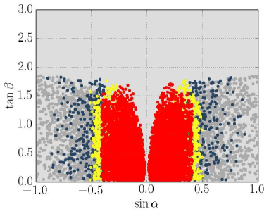
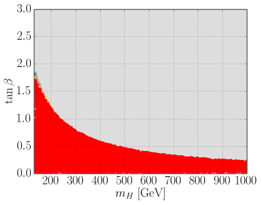

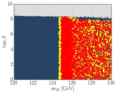
The results are presented in Fig. 10 in terms of two–dimensional scatter plots in the three scan parameters. The point distribution in the (, ) plane shown in Fig. 10(a) neatly resembles the features of Fig. 9 discussed above: Small mixings are forbidden from the requirement of vacuum stability, while the maximal value for the mixing angle, , is limited by the Higgs signal rate observables. Fig. 10(b) illustrates how the upper limit on , which stems from the perturbativity requirement of , roughly follows the expected scaling, cf. Eq. (30). Finally, we can easily recognize the upper limit on the mixing angle from the constraint and the perturbativity requirement of , cf. Fig. 3, in the point distribution in the (, ) plane shown in Fig. 10(c). These constraints provide the most stringent upper limit on for Higgs masses . At lower Higgs masses, the upper limit is set by the Higgs signal rate measurements and exclusion limits from Higgs searches at the LHC, cf. Fig. 8. Here it is interesting to see that the favored region at Higgs masses between and is more restricted than at higher Higgs masses. Two effects play a role here: Firstly, the lower limit on from the vacuum stability requirement is stronger than at larger Higgs masses; And secondly, the heavy Higgs boson lies still in the vicinity of the discovered Higgs state, such that their signal rates are combined in the , and channels, where the mass resolution is poor. In total, these channels however favor a slightly lower signal strength than obtained for a SM Higgs, thus the fit slightly prefers larger Higgs masses , where the signal rates are not added for these observables within HiggsSignals, cf. also Fig. 7.
We now turn to the discussion of the collider phenomenology of the high mass region. Experimentally, the model can be probed by searches for a SM–like Higgs boson with a reduced signal rate and total decay widths, or by direct searches for the Higgs-to-Higgs decay mode , where is the light Higgs boson at around .
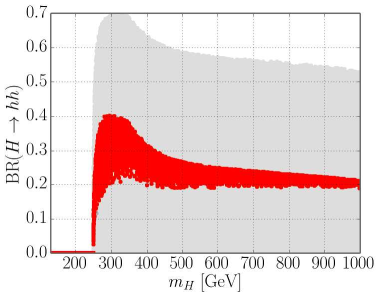
We show the allowed values of the branching ratio , given by Eq. (II.1), in Fig. 11. In Fig. 11(a) we show the dependence on exemplarily for fixed Higgs masses , whereas the full dependence is displayed in Fig. 11(b), using the same color code as above. We observe that the maximal values of are , reached for large, positive values Pruna:2013bma , and low Higgs masses . At higher Higgs masses the branching ratio is around or slightly higher.


The LHC production cross section of the heavier Higgs boson is given by the SM Higgs production cross section multiplied by . For convenience, we introduce the rate scale factors Pruna:2013bma
| (43) | ||||
| (44) |
for the heavy Higgs collider processes leading to SM particles or two light Higgs bosons in the final state, respectively. Here, comprises all possible Higgs decay modes to SM particles. Note, that corresponds to the inclusive heavy Higgs production rate, normalized to the inclusive SM Higgs production rate Dittmaier:2011ti ; Dittmaier:2012vm ; Heinemeyer:2013tqa .
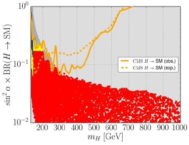
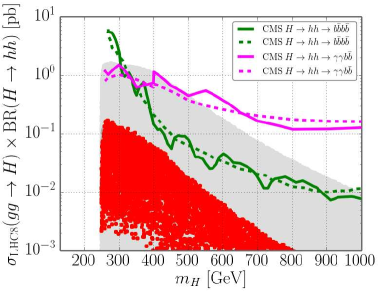
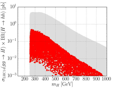
The predicted signal rates normalized to the SM production cross section, Eqs. (43) and (44), are shown as a function of the Higgs mass for the high mass region in Fig. 12. We furthermore display the current exclusion limits from the latest CMS combination of SM Higgs searches CMS:aya , as well as from direct searches for the process with CMS:2014ipa and CMS:2014eda final states. We see that at the current stage, the experimental searches with SM-like final states yield important constraints for . As discussed above, at larger masses the upper limit on the mixing angle, and thus on the maximal production cross section, stems either from or from perturbativity. Note, that the displayed CMS limit from the SM Higgs search combination CMS:aya is only based on of and of data, thus not exploiting the full available data from LHC run 1. Obviously, future LHC searches for a SM-like Higgs boson with reduced couplings in the full accessible mass range will play an important role in probing the singlet extended SM. The direct searches for the process carried out by CMS in the final states CMS:2014ipa and, in particular, CMS:2014eda draw near to the allowed region at masses . While they do not yield any relevant constraints at the current stage, these searches will become important in this model in the upcoming LHC runs, as they are complementary to the SM-like Higgs searches. For reference, we also provide the predicted LHC signal cross section for both the SM Higgs signatures and signature for CM energies of and in Fig. 13. Note that, as discussed earlier (see footnote 7), we do not include effects from the interference with the Higgs boson at in these predictions.
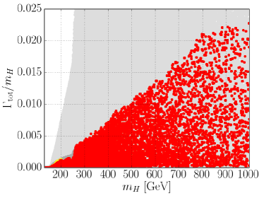
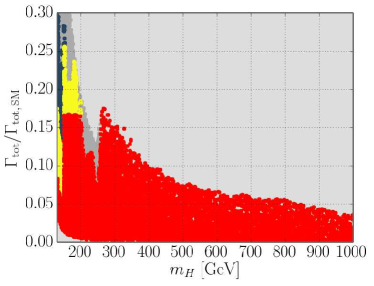

In general, the total width of the heavy Higgs boson is of high interest for collider searches. In the SM, the width of the SM Higgs boson rapidly rises with its mass. In Ref. Pruna:2013bma it was shown that in the singlet extended SM the total width of the heavy resonance, , is highly suppressed due to the small mixing angle required. The same behavior is observed here. We show the ratio , as well as the suppression of the width, , in Fig. 14. We see that the total width of the heavy Higgs only amounts to up to at lower masses , while it is even further suppressed to below of the SM Higgs width for masses . At , the total width is still below . In comparison to SM Higgs boson of the same mass, the total width of these resonances is therefore highly suppressed, which promises to enhance the validity of a narrow width approximation in this mass range.131313See e.g. Ref. Goria:2011wa for the discussion of finite width effects for SM-like Higgs bosons in the mass range .
For completeness, we show the allowed parameter space in the () and () planes in Fig. 15. If these predictions are taken as independent input parameters in future Higgs boson collider searches, a direct comparison with the experimental results renders additional constraints and — in case of a discovery — could possibly lead to an exclusion of the entire model.
IV.2 Low mass region
We now consider the low mass region, i.e. we set the heavy Higgs mass to and investigate the parameter space with . In contrast to the high mass region, results from LEP searches play an important role in this part of parameter space. As discussed in Section III.3, we here do not apply limits from RGE running of the couplings. Before constraints from the signal rates are taken into account, this a priori leads to much larger allowed values for , where the upper limit on stems from perturbative unitarity, cf. Fig. 1. However, whenever the additional decay is kinematically allowed, values generally result in large branching ratios for this channel, cf. Fig. 5(a). This immediately imposes a quite strong suppression of the SM decays of the heavy Higgs state, leading to strong bounds on the minimal value from the signal rates, cf. Section III.6. However, we should keep in mind that in parameter regions where , the branching ratio for decreases significantly, thus restoring the signal strength of the heavy Higgs boson to times the SM Higgs signal strength. In the mass range where the additional decay is not allowed and up to values of , the strongest limits on the mixing angle stem from LEP Higgs searches in the channel Schael:2006cr . For larger Higgs masses, the Higgs signal rates yield stricter limits on than the exclusion limits from LEP and LHC, cf. also Fig. 7. We have summarized our finding in the low mass scenario in Tab. 3.
| 0.410 | 0.918 | 8.4 | – | |
| – | ||||
| – | ||||
| – | – | |||
| – | – | |||
| – | – | |||
| 0.21 | ||||
| 0.20 | ||||
| 0.18 | ||||
| 0.988 | 0.998 | 33.6 | 0.16 | |
| 0.993 | 0.998 | 50.4 | 0.12 | |
| 0.997 | 0.998 | 100.8 | 0.08 |
We now turn to the discussion of the full scan. In order to highlight the importance of LEP constraints in the low mass region, we employ the following color coding for the plots:
-
•
Light gray: points which fail theoretical constraints.
-
•
Dark gray: points which are excluded by LHC Higgs searches.
-
•
Blue: points allowed by LHC Higgs searches, but excluded by by LEP searches.
-
•
Dark green: points consistent with LEP constraints within .
-
•
Light green: points consistent with LEP constraints within .
-
•
Yellow: points favored within in the global fit (HiggsSignals + LEP ).
-
•
red: points favored within in the global fit (HiggsSignals + LEP ).
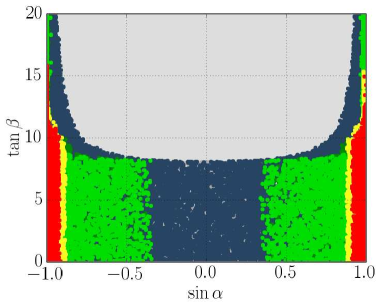
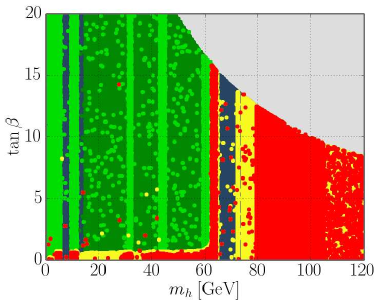
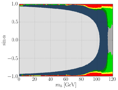
The results are shown in Fig. 16 in terms of two-dimensional scatter plots in the scan parameters. In Fig. 16(c), we see that most parameter points allowed by the global fit at the level are found for and . For lower Higgs masses the mixing angle is constrained to values very close to the decoupling scenario (). The LEP limits are particularly strong in the mass region between and , cf. Fig. 4(a), such that only a few valid points are found here, as can be seen best in Fig. 16(b). The semi-oval exclusion region in Figs. 16(a) and 16(c) for large values and low values, respectively, corresponds to a deviation in the electroweak oblique parameters , and .
In Fig. 16(b), we observe a drastic change in the distribution of allowed parameter points when going to Higgs masses , where the decay mode becomes kinematically accessible. As discussed earlier in Section III.6, cf. Fig. 5, the decay easily becomes the dominant decay mode if , unless the mixing angle is very close to . Hence, for , most of the allowed points are found for small values of , since the Higgs signal rates favor small values of . At larger Higgs masses, , the favored points are equally distributed over the entire range allowed by perturbative unitarity.

It is interesting to investigate the allowed range of the signal rate in dependence of the light Higgs mass. This is shown in Fig. 17(a), where the signal rate is normalized to the SM Higgs boson production. Note, that due to the LEP constraints, the favored points feature a mixing angle and thus the displayed signal rate closely resembles . We see that the maximally allowed signal rate is about and is roughly independent on the light Higgs mass141414The reason why the density of allowed points still depends strongly on is that regions which are strongly constrained by LEP searches require a large fine-tuning of to render allowed points. . This upper limit solely stems from the observed signal rates of the SM–like Higgs boson at . These constraints therefore also limit the total width of the heavy Higgs at to values , being in the vicinity of the SM total width of .
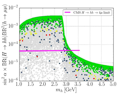
We now discuss the case of very low Higgs masses, . Here, the LEP constraints stem from the decay-mode independent analysis of by OPAL Abbiendi:2002qp , yielding a slightly weaker limit on the mixing angle, , than at larger masses, cf. Fig. 4(a). In the mass region , the branching fraction for the light Higgs decay amounts between , thus allowing to search for the signature at the LHC. We show the predicted signal rate for this signature151515We consider here only the Higgs production via gluon gluon fusion. for the LHC at a center-of-mass energy of in Fig. 17(b). A search for this signature has been performed by CMS CMS:2013lea , yielding the observed upper limit161616This exclusion limit is not provided with HiggsBounds-4.2.0, because the expected limit from the CMS analysis is not publicly available. displayed as magenta line in the figure. As can be seen, the CMS limit provides competitive constraints in this parameter region, excluding a sizable amount of the parameter region favored by the global fit. Future LHC searches for the signature therefore have a good discovery potential in this mass region. Other final states, composed of leptons, strange or charm quarks, could be exploited at a future linear collider like the ILC.
A very light Higgs boson with mass values up to the threshold can also be probed at -factories in the radiative decay Wilczek:1977zn , with successive decay of the light Higgs boson to -lepton, muon or hadron pairs. Here, we provide a rough estimate of the present constraints.
The decay rate for the bound state to the Higgs-photon final state (normalized to the decay rate of ) is given by Wilczek:1977zn
| (45) |
where is the Fermi constant, the bottom quark mass, the fine-structure constant and Agashe:2014kda . The factor represents higher-order corrections. The one-loop QCD corrections have been calculated in Ref. Vysotsky:1980cz ; Nason:1986tr and are known to reduce the leading-order estimate by up to , see Ref. Gunion:1989we for an extended discussion. In our model, the rescaling factor of the bottom Yukawa coupling of the light Higgs is simply given by .
Recent experimental searches have been carried out by BaBar Aubert:2009cka ; Lees:2012te ; Aubert:2009cp ; Lees:2012iw ; Lees:2013vuj and CLEO Love:2008aa , focussing on the search for a light -odd Higgs boson motivated by certain next-to-minimal supersymmetric standard model (NMSSM) scenarios Dermisek:2005ar ; Dermisek:2006py ; Domingo:2008rr . The upper limits on the branching fraction of these search signatures are typically of and are listed for representative values of the light Higgs mass in Tab. 4 (cf. also Refs. Echenard:2012hq ; Domingo:2010am ; Bevan:2014iga for more details). Generally, these limits underlie large statistical fluctuations, thus we prefer to use a roughly estimated mean value and indicate this by a ’‘ in front of the quoted number. Using the SM Higgs boson branching ratios for , , and in this mass region, we can infer a upper limit on the rescaling factor of the bottom Yukawa coupling, , which is listed in Tab. 4. If this upper limit is below , we furthermore quote the resulting lower limit on the mixing angle in the table. The resulting limits cannot compete with those obtained from direct LEP searches, however, future -physics facilities such as the Belle II experiment at the Super KEKB accelerator Abe:2010gxa will be able to probe the yet unexcluded region.
| upper limit on , | ||||||
| Lees:2012iw | Lees:2012te | Lees:2013vuj | Lees:2013vuj | (upper limit) | (lower limit) | |
| – | – | |||||
| – | – | |||||
| – | – | |||||
| – | ||||||
| – | ||||||
| – | ||||||
| – | ||||||
Finally, we want to comment that despite of the quite strong constraints in the low mass region, a substantial number of low mass Higgs bosons could already have been directly produced at the LHC. Table 5 exemplarily lists the maximally allowed LHC cross sections for direct production in gluon gluon fusion for a selected range of light Higgs masses at CM energies of and .171717We thank M. Grazzini for providing us with the production cross sections for . We encourage the LHC experiments to explore the feasibility of experimental searches within the low mass region and to potentially extend the searches for directly produced scalars into this mass range.
| 3.28 | 8.40 | |
| 3.24 | 8.12 | |
| 6.12 | 14.96 | |
| 6.82 | 16.26 | |
| 2.33 | 5.41 | |
| 2.97 | 6.73 | |
| 0.63 | 1.38 | |
| 0.45 | 0.96 | |
| 0.74 | 1.50 |
IV.3 Intermediate mass region
For the intermediate mass region, which contains the special case of mass-degenerate Higgs states, we treat both Higgs masses as free parameters in the fit, . Note, that the following discussion is based on a few simplifying assumptions about overlapping Higgs signals in the experimental analyses. It should be clear that a precise investigation of the near mass-degenerate Higgs scenario can only be performed by analyzing the LHC data directly and is thus restricted to be done by the experimental collaborations (see e.g. Ref. Khachatryan:2014ira for such an analysis). Nevertheless, we want to point out this interesting possibility here and encourage the LHC experiments for further investigations.
If the Higgs states have very similar masses, their signals cannot be clearly distinguished in the experimental analyses and (to first approximation) the sum of the signal rates has to be considered for the comparison with the measured rates. Moreover, the observed peak in the invariant mass distribution in the and channels, which is fitted to determine the Higgs mass, would actually comprise two (partially) overlapping Higgs resonances, where the height of each resonance is governed by the corresponding signal strength. Therefore, for each Higgs analysis where a mass measurement has been performed, cf. Tab. 1, we calculate a signal strength weighted mean value of the Higgs masses181818Testing overlapping signals of multiple Higgs bosons against mass measurements by employing a mass average calculation is the default procedure in HiggsSignals since version 1.3.0.,
| (46) |
to be tested against the measurement, where the SM normalized signal strengths are given by
| (47) |
Here, denotes the mass value hypothesized by the experiment during to signal rate measurement. The index runs over all signal channels, i.e. Higgs production times decay mode, considered in the experimental analysis, and denotes the corresponding efficiencies. The predicted cross sections and partial widths are obtained from rescaling the respective SM quantities Dittmaier:2011ti ; Dittmaier:2012vm ; Heinemeyer:2013tqa by and for and , respectively. As mentioned earlier in Section III.6, the SM normalized signal strengths contain a slight mass dependence191919This mass dependence is neglected per default in HiggsSignals since additional complications arise if theoretical mass uncertainties are present. This is however not the case here, since we use the Higgs masses directly as input parameters. The evaluation of the signal strength according to Eq. (47) can be activated in HiggsSignals by setting normalize_rates_to_reference_position=.True. in the file usefulbits_HS.f90. since the SM cross sections and branching ratios are not constant over the relevant mass range.
| – | |||
| – | |||
| – | – | ||
| – | |||
| – | |||
| – | |||
| – | |||
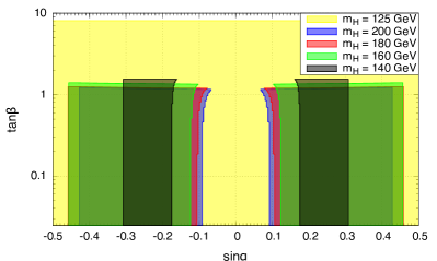
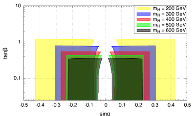
We present limits on and for various choices of the Higgs mass in the intermediate mass region in Tab. 6. We fixed the other Higgs mass to . Depending on whether or not the Higgs mass is larger than , we obtain either an upper or lower limit on from the LHC Higgs search exclusion limits or signal rate measurements, which are listed separately. In the case of nearly degenerate Higgs masses, , no limit on can be obtained, since the Higgs signals completely overlap. We find that no limits from exclusions from Higgs searches can be obtained for Higgs masses within and . Moreover, the limits inferred from the signal rates become weaker the closer is to due to the signal overlap. In the full intermediate mass region, the limits inferred from the Higgs signal rates supersede the limits obtained from null results in LHC Higgs searches.
The upper limits on listed in Tab. 6 correspond to the perturbative unitarity bound (cf. Fig. 1). Similarly as in the low mass region, we do not impose constraints from perturbativity and vacuum stability at a high energy scale here. If these were additionally required, would be limited to values for . For lower Higgs masses no valid points would be found. It should be noted, however, that the collider phenomenology does not depend on in the intermediate mass region, since Higgs-to-Higgs decays are kinematically not accessible.
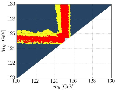


The results from the full four-dimensional scan are presented in Fig. 18 in terms of two-dimensional scatter plots, using the same color coding as in the high mass region (see e.g. Fig. 10). The correlation between the two Higgs masses, Fig. 18(a), shows that allowed parameter points with Higgs bosons in the full intermediate mass region are found, however, at least one of the Higgs masses is always required to be roughly between and . We can furthermore learn from Figs. 18(c) and 18(d), that allowed points with one Higgs mass being below (above ) feature values close to , such that the other Higgs state at around has SM Higgs–like signal strengths. In the near-degenerate case, , all mixing angles are allowed and the model appears indistinguishable from the SM at current collider experiments.
Fig. 18 also shows the correlations of with the mixing angle , Fig. 18(b), and the Higgs masses, Figs. 18(e) and 18(f). As stated earlier, does not influence the collider phenomenology in the intermediate mass range, thus we find allowed parameter points in the full range up to the maximal value given by perturbative unitarity.
A direct search for the second Higgs boson in the intermediate mass region at the LHC seems challenging. Even if the mass splitting between the two Higgs states is large enough to be resolved by the experimental analyses, we expect the second resonance to be much smaller than the established signal. Nevertheless we would like to encourage the LHC experiments to perform dedicated resonance searches, in particular in the mass region slightly above the current signal, , since in this case larger values of the mixing angle are still allowed while an improvement of the vacuum stability at the high–scale may be obtained. More promising prospects to resolve the near mass–degenerate Higgs scenario have future experimental facilities like the ILC Asner:2013psa ; Dawson:2013bba or a muon collider Alexahin:2013ojp ; Dawson:2013bba , where the latter provides excellent opportunities to measure the mass and the total width of the discovered Higgs boson via a line-shape scan.
V Conclusions
In this work, we have investigated the theoretical and experimental limits on the parameter space of a real singlet extension of the SM Higgs sector, considering mass values of the second Higgs boson ranging from to , i.e. within the accessible mass range of past, current and future collider experiments. This study complements a previous work Pruna:2013bma that was restricted to and moreover did not include constraints from direct Higgs collider searches. In the present work, either the heavy or the light Higgs state can take the role of the discovered SM-like Higgs boson at . We found that up to Higgs masses , exclusion limits from direct Higgs collider searches at LEP and the LHC, as well as the requirement of consistency with the measured SM-like Higgs signal rates pose quite strong constraints. At higher Higgs masses, strong limits stem from electroweak precision observables, in particular from the boson mass calculated at NLO, as well as from requiring perturbativity of the couplings and vacuum stability. The latter two are tested both at the electroweak scale and at a high scale using the -functions of the theory (see e.g. Ref. Pruna:2013bma and references therein).
We performed a exhaustive scan in the three model parameters — specified by the Higgs mixing angle, the second Higgs mass and the ratio of the Higgs VEVs — and provided a detailed discussion of the viable parameter space and the relative importance of the various constraints. We translated these results into predictions for collider observables for the second yet undiscovered Higgs boson, which are currently investigated by the LHC experiments. In particular, we focussed on the global rescaling factor for the SM Higgs decay modes, the signal rate for the Higgs-to-Higgs decay signature as well as the total width of the new scalar. A typical feature of the model is that the total width of the new scalar is quite suppressed with respect to the SM Higgs boson at such masses. At very light Higgs boson masses below we found that new results from LHC searches for the signature are complementary to LEP Higgs searches and thus probe an unexplored parameter region. Also future -factories should be able to probe these parameter regions through the decay .
We furthermore investigated the intermediate mass region, where both Higgs masses are between and , and discussed some of the experimental challenges in probing this scenario. Dedicated LHC searches for an additional resonance in the invariant mass spectra of the (see Ref. Khachatryan:2014ira for a CMS analysis) and channel in the vicinity of the discovered Higgs boson as well as future precision experiments at the ILC or a muon collider may shed more light onto this case.
The discovery of additional Higgs states is one of the main goals of the upcoming runs of the LHC. In this model, two distinct and complementary signatures of the second Higgs state arise. Firstly, the decay signature, where the best sensitivity for the LHC is obtained for heavy Higgs masses between and roughly . These signatures have been recently explored by ATLAS and CMS CMS:2014ipa ; CMS:2014eda ; atlHtohh but the analyses are not yet sensitive to constrain the parameter space. Secondly, Higgs searches designed for a SM Higgs boson are sensitive probes of the parameter space. We strongly encourage the experimental collaborations to continue these searches in the full accessible mass range. However, some of the features of the second Higgs state discussed in this work, such as the strong reduction of the total width, should be taken into account in upcoming analyses. Finally, we hope that the predictions of LHC signal cross sections at a CM energy of will be found useful for designing some interesting benchmark points for the experimental analyses of this model.
Acknowledgements
We thank Klaus Desch and Sven Heinemeyer for inspiring remarks and for motivating us to perform this study. We furthermore acknowledge helpful discussions with Philip Bechtle, Howie Haber, Antonio Morais, Marco Sampaio, Rui Santos and Martin Wiebusch. The code for testing perturbative unitarity has been adapted from Ref. Pruna:2013bma . TS is supported in part by U.S. Department of Energy grant number DE-FG02-04ER41286, and in part by a Feodor-Lynen research fellowship sponsored by the Alexander von Humboldt Foundation.
Appendix A Minimization and vacuum stability conditions
In this appendix we briefly guide the reader through the steps from Eq. (8) to Eq. (10), using the definition of the scalar fields given in Eq. (12). We basically follow the discussion as presented in Ref. Pruna:2013bma .
With the definition of the VEVs according to Eq. (12), the extrema of are determined using the following set of equations:
| (48) | ||||
| (49) |
The physically interesting solutions have :
| (50) | |||||
| (51) |
Alternatively, we use Eq. (48) to eliminate and , leading to
| (52) |
Since the denominator in Eqs. (50)–(51) is always positive (assuming that the potential is well-defined), the numerators need to be positive as well in order to guarantee a positive-definite non-vanishing solution for and .
Appendix B RGEs for SM gauge couplings and the top quark Yukawa coupling
This section basically follows the discussion in Ref. Pruna:2013bma . In the SM, all one-loop RGEs for gauge couplings are of the form
The exact analytic solution for this equation is given by
| (54) |
where for we have
For positive values of , the coupling reaches the Landau pole when the denominator in Eq. (54) goes to 0; for negative values, for .
The Yukawa coupling terms are in turn given by
with the solution
with , where defines the initial value. For the top quark Yukawa coupling we have
However, taking the explicit scale-dependence of the SM gauge couplings into account, the above solution needs to be modified such that is replaced by . In this work we chose to solve the RGE of the top quark Yukawa coupling numerically.
References
- (1) ATLAS Collaboration, G. Aad et al., Phys.Lett. B716, 1 (2012), arXiv:1207.7214.
- (2) CMS Collaboration, S. Chatrchyan et al., Phys.Lett. B716, 30 (2012), arXiv:1207.7235.
- (3) ATLAS Collaboration, G. Aad et al., Phys.Lett. B726, 120 (2013), arXiv:1307.1432.
- (4) ATLAS Collaboration, G. Aad et al., (2014), arXiv:1408.7084.
- (5) ATLAS Collaboration, G. Aad et al., (2014), arXiv:1408.5191.
- (6) ATLAS Collaboration, G. Aad et al., (2014), arXiv:1409.6212.
- (7) CMS Collaboration, V. Khachatryan et al., Eur.Phys.J. C74, 3076 (2014), arXiv:1407.0558.
- (8) CMS Collaboration, S. Chatrchyan et al., Nature Phys. 10 (2014), arXiv:1401.6527.
- (9) CMS Collaboration, S. Chatrchyan et al., Phys.Rev. D89, 092007 (2014), arXiv:1312.5353.
- (10) CMS Collaboration, S. Chatrchyan et al., JHEP 1401, 096 (2014), arXiv:1312.1129.
- (11) P. W. Higgs, Phys.Lett. 12, 132 (1964).
- (12) P. W. Higgs, Phys.Rev.Lett. 13, 508 (1964).
- (13) F. Englert and R. Brout, Phys.Rev.Lett. 13, 321 (1964).
- (14) G. Guralnik, C. Hagen, and T. Kibble, Phys.Rev.Lett. 13, 585 (1964).
- (15) T. Kibble, Phys.Rev. 155, 1554 (1967).
- (16) ATLAS Collaboration, G. Aad et al., Phys.Rev. D90, 052004 (2014), arXiv:1406.3827.
- (17) CMS Collaboration, (2014), CMS-PAS-HIG-14-009.
- (18) D. Asner et al., (2013), arXiv:1310.0763.
- (19) R. Schabinger and J. D. Wells, Phys.Rev. D72, 093007 (2005), arXiv:hep-ph/0509209.
- (20) B. Patt and F. Wilczek, (2006), arXiv:hep-ph/0605188.
- (21) V. Barger, P. Langacker, M. McCaskey, M. J. Ramsey-Musolf, and G. Shaughnessy, Phys.Rev. D77, 035005 (2008), arXiv:0706.4311.
- (22) G. Bhattacharyya, G. C. Branco, and S. Nandi, Phys.Rev. D77, 117701 (2008), arXiv:0712.2693.
- (23) S. Dawson and W. Yan, Phys.Rev. D79, 095002 (2009), arXiv:0904.2005.
- (24) S. Bock et al., Phys.Lett. B694, 44 (2010), arXiv:1007.2645.
- (25) P. J. Fox, D. Tucker-Smith, and N. Weiner, JHEP 1106, 127 (2011), arXiv:1104.5450.
- (26) C. Englert, T. Plehn, D. Zerwas, and P. M. Zerwas, Phys.Lett. B703, 298 (2011), arXiv:1106.3097.
- (27) C. Englert, J. Jaeckel, E. Re, and M. Spannowsky, Phys.Rev. D85, 035008 (2012), arXiv:1111.1719.
- (28) B. Batell, S. Gori, and L.-T. Wang, JHEP 1206, 172 (2012), arXiv:1112.5180.
- (29) C. Englert, T. Plehn, M. Rauch, D. Zerwas, and P. M. Zerwas, Phys.Lett. B707, 512 (2012), arXiv:1112.3007.
- (30) R. S. Gupta and J. D. Wells, Phys.Lett. B710, 154 (2012), arXiv:1110.0824.
- (31) M. J. Dolan, C. Englert, and M. Spannowsky, Phys.Rev. D87, 055002 (2013), arXiv:1210.8166.
- (32) D. Bertolini and M. McCullough, JHEP 1212, 118 (2012), arXiv:1207.4209.
- (33) B. Batell, D. McKeen, and M. Pospelov, JHEP 1210, 104 (2012), arXiv:1207.6252.
- (34) D. Lopez-Val, T. Plehn, and M. Rauch, JHEP 1310, 134 (2013), arXiv:1308.1979.
- (35) The LHC Higgs Cross Section Working Group, S. Heinemeyer et al., (2013), arXiv:1307.1347.
- (36) R. S. Chivukula, A. Farzinnia, J. Ren, and E. H. Simmons, Phys.Rev. D88, 075020 (2013), arXiv:1307.1064.
- (37) C. Englert and M. McCullough, JHEP 1307, 168 (2013), arXiv:1303.1526.
- (38) B. Cooper, N. Konstantinidis, L. Lambourne, and D. Wardrope, Phys.Rev. D88, 114005 (2013), arXiv:1307.0407.
- (39) C. Caillol, B. Clerbaux, J.-M. Frere, and S. Mollet, Eur.Phys.J.Plus 129, 93 (2014), arXiv:1304.0386.
- (40) R. Coimbra, M. O. Sampaio, and R. Santos, Eur.Phys.J. C73, 2428 (2013), arXiv:1301.2599.
- (41) G. M. Pruna and T. Robens, Phys.Rev. D88, 115012 (2013), arXiv:1303.1150.
- (42) S. Dawson et al., (2013), arXiv:1310.8361.
- (43) D. Lopez-Val and T. Robens, Phys.Rev. D90, 114018 (2014), arXiv:1406.1043.
- (44) C. Englert and M. Spannowsky, Phys.Rev. D90, 053003 (2014), arXiv:1405.0285.
- (45) C. Englert, Y. Soreq, and M. Spannowsky, (2014), arXiv:1410.5440.
- (46) C.-Y. Chen, S. Dawson, and I. Lewis, (2014), arXiv:1410.5488.
- (47) D. Karabacak, S. Nandi, and S. K. Rai, Phys.Lett. B737, 341 (2014), arXiv:1405.0476.
- (48) S. Profumo, M. J. Ramsey-Musolf, C. L. Wainwright, and P. Winslow, (2014), arXiv:1407.5342.
- (49) L. Basso, S. Moretti, and G. M. Pruna, Phys.Rev. D82, 055018 (2010), arXiv:1004.3039.
- (50) M. J. Strassler and K. M. Zurek, Phys.Lett. B651, 374 (2007), arXiv:hep-ph/0604261.
- (51) M. J. Strassler and K. M. Zurek, Phys.Lett. B661, 263 (2008), arXiv:hep-ph/0605193.
- (52) P. Bechtle, O. Brein, S. Heinemeyer, G. Weiglein, and K. E. Williams, Comput. Phys. Commun. 181, 138 (2010), arXiv:0811.4169.
- (53) P. Bechtle, O. Brein, S. Heinemeyer, G. Weiglein, and K. E. Williams, Comput. Phys. Commun. 182, 2605 (2011), arXiv:1102.1898.
- (54) P. Bechtle et al., PoS CHARGED2012, 024 (2012), arXiv:1301.2345.
- (55) P. Bechtle et al., Eur. Phys. J. C 74, 2693 (2013), arXiv:1311.0055.
- (56) P. Bechtle, S. Heinemeyer, O. Stål, T. Stefaniak, and G. Weiglein, Eur.Phys.J. C74, 2711 (2014), arXiv:1305.1933.
- (57) P. Bechtle, S. Heinemeyer, O. Stål, T. Stefaniak, and G. Weiglein, JHEP 1411, 039 (2014), arXiv:1403.1582.
- (58) M. Bowen, Y. Cui, and J. D. Wells, JHEP 0703, 036 (2007), arXiv:hep-ph/0701035.
- (59) G. Altarelli and R. Barbieri, Phys. Lett. B 253, 161 (1991).
- (60) M. E. Peskin and T. Takeuchi, Phys.Rev.Lett. 65, 964 (1990).
- (61) M. E. Peskin and T. Takeuchi, Phys.Rev. D46, 381 (1992).
- (62) I. Maksymyk, C. Burgess, and D. London, Phys.Rev. D50, 529 (1994), arXiv:hep-ph/9306267.
- (63) B. W. Lee, C. Quigg, and H. Thacker, Phys.Rev. D16, 1519 (1977).
- (64) M. Luscher and P. Weisz, Phys.Lett. B212, 472 (1988).
- (65) L. Basso, A. Belyaev, S. Moretti, and G. Pruna, Phys.Rev. D81, 095018 (2010), arXiv:1002.1939.
- (66) R. N. Lerner and J. McDonald, Phys.Rev. D80, 123507 (2009), arXiv:0909.0520.
- (67) G. Degrassi et al., JHEP 1208, 098 (2012), arXiv:1205.6497.
- (68) R. Costa, A. P. Morais, M. O. P. Sampaio, and R. Santos, (2014), arXiv:1411.4048.
- (69) ALEPH Collaboration, DELPHI Collaboration, L3 Collaboration, OPAL Collaboration, LEP Electroweak Working Group, J. Alcaraz et al., (2006), arXiv:hep-ex/0612034.
- (70) CDF Collaboration, T. Aaltonen et al., Phys.Rev.Lett. 108, 151803 (2012), arXiv:1203.0275.
- (71) D0 Collaboration, V. M. Abazov et al., Phys.Rev. D89, 012005 (2014), arXiv:1310.8628.
- (72) M. Awramik, M. Czakon, A. Freitas, and G. Weiglein, Phys.Rev. D69, 053006 (2004), arXiv:hep-ph/0311148.
- (73) Gfitter Group, M. Baak et al., Eur.Phys.J. C74, 3046 (2014), arXiv:1407.3792.
- (74) K. Hagiwara, S. Matsumoto, D. Haidt, and C. Kim, Z.Phys. C64, 559 (1994), arXiv:hep-ph/9409380.
- (75) S. Goria, G. Passarino, and D. Rosco, Nucl.Phys. B864, 530 (2012), arXiv:1112.5517.
- (76) K. Hagiwara et al., Phys.Rev. D73, 055005 (2006), arXiv:hep-ph/0512260.
- (77) C. Uhlemann and N. Kauer, Nucl.Phys. B814, 195 (2009), arXiv:0807.4112.
- (78) D. Wiesler, DESY-THESIS-2012-048.
- (79) E. Maina, (2015), arXiv:1501.02139.
- (80) H. E. Logan, (2014), arXiv:1412.7577.
- (81) J. Kalinowski, W. Kilian, J. Reuter, T. Robens, and K. Rolbiecki, JHEP 0810, 090 (2008), arXiv:0809.3997.
- (82) N. Kauer and G. Passarino, JHEP 1208, 116 (2012), arXiv:1206.4803.
- (83) CMS Collaboration, S. Chatrchyan et al., Phys.Lett. B710, 26 (2012), arXiv:1202.1488.
- (84) ATLAS Collaboration, G. Aad et al., Phys.Rev. D86, 032003 (2012), arXiv:1207.0319.
- (85) CMS Collaboration, (2012), CMS-PAS-HIG-12-045.
- (86) ATLAS Collaboration, (2013), ATLAS-CONF-2013-013, ATLAS-COM-CONF-2013-018.
- (87) CMS Collaboration, S. Chatrchyan et al., Phys.Rev.Lett. 108, 111804 (2012), arXiv:1202.1997.
- (88) CMS Collaboration, (2013), CMS-PAS-HIG-13-002.
- (89) ATLAS Collaboration, (2013), ATLAS-CONF-2013-030, ATLAS-COM-CONF-2013-028.
- (90) CMS Collaboration, (2013), CMS-PAS-HIG-13-003.
- (91) ATLAS Collaboration, G. Aad et al., Phys.Rev.Lett. 113, 171801 (2014), arXiv:1407.6583.
- (92) ALEPH Collaboration, DELPHI Collaboration, L3 Collaboration, OPAL Collaboration, LEP Working Group for Higgs Boson Searches, S. Schael et al., Eur.Phys.J. C47, 547 (2006), arXiv:hep-ex/0602042.
- (93) OPAL Collaboration, G. Abbiendi et al., Eur.Phys.J. C27, 311 (2003), arXiv:hep-ex/0206022.
- (94) CMS Collaboration, CMS Collaboration, (2013), CMS-PAS-HIG-13-010.
- (95) CMS Collaboration, CMS Collaboration, (2013), CMS-PAS-HIG-13-025.
- (96) ATLAS collaboration, (2014), ATLAS-CONF-2014-060, ATLAS-COM-CONF-2014-078.
- (97) ATLAS collaboration, (2014), ATLAS-CONF-2014-061, ATLAS-COM-CONF-2014-080.
- (98) Y. Alexahin et al., (2013), arXiv:1308.2143.
- (99) CMS Collaboration, CMS Collaboration, (2014), CMS-PAS-HIG-13-032.
- (100) CMS Collaboration, CMS Collaboration, (2014), CMS-PAS-HIG-14-013.
- (101) LHC Higgs Cross Section Working Group, S. Dittmaier et al., (2011), arXiv:1101.0593.
- (102) S. Dittmaier et al., (2012), arXiv:1201.3084.
- (103) F. Wilczek, Phys.Rev.Lett. 39, 1304 (1977).
- (104) Particle Data Group, K. Olive et al., Chin.Phys. C38, 090001 (2014).
- (105) M. Vysotsky, Phys.Lett. B97, 159 (1980).
- (106) P. Nason, Phys.Lett. B175, 223 (1986).
- (107) J. F. Gunion, H. E. Haber, G. L. Kane, and S. Dawson, Front.Phys. 80, 1 (2000).
- (108) BaBar Collaboration, B. Aubert et al., Phys.Rev.Lett. 103, 181801 (2009), arXiv:0906.2219.
- (109) BaBar Collaboration, J. Lees et al., Phys.Rev. D88, 071102 (2013), arXiv:1210.5669.
- (110) BaBar Collaboration, B. Aubert et al., Phys.Rev.Lett. 103, 081803 (2009), arXiv:0905.4539.
- (111) BaBar collaboration, J. Lees et al., Phys.Rev. D87, 031102 (2013), arXiv:1210.0287.
- (112) BaBar Collaboration, J. Lees et al., Phys.Rev. D88, 031701 (2013), arXiv:1307.5306.
- (113) CLEO Collaboration, W. Love et al., Phys.Rev.Lett. 101, 151802 (2008), arXiv:0807.1427.
- (114) R. Dermisek and J. F. Gunion, Phys.Rev.Lett. 95, 041801 (2005), arXiv:hep-ph/0502105.
- (115) R. Dermisek, J. F. Gunion, and B. McElrath, Phys.Rev. D76, 051105 (2007), arXiv:hep-ph/0612031.
- (116) F. Domingo, U. Ellwanger, E. Fullana, C. Hugonie, and M.-A. Sanchis-Lozano, JHEP 0901, 061 (2009), arXiv:0810.4736.
- (117) B. Echenard, Adv.High Energy Phys. 2012, 514014 (2012), arXiv:1209.1143.
- (118) F. Domingo, JHEP 1104, 016 (2011), arXiv:1010.4701.
- (119) BaBar Collaboration, Belle Collaboration, A. Bevan et al., Eur.Phys.J. C74, 3026 (2014), arXiv:1406.6311.
- (120) Belle-II Collaboration, T. Abe et al., (2010), arXiv:1011.0352.
- (121) M. Grazzini. Private communication.
- (122) ATLAS collaboration, (2014), ATLAS-CONF-2014-005, ATLAS-COM-CONF-2014-007.