Extended distribution functions for our Galaxy
Abstract
We extend models of our Galaxy based on distribution functions (dfs) that are analytic functions of the action integrals to extended distribution functions (edfs), which have an analytic dependence on metallicity as well. We use a simple, but physically-motivated, functional forms for the metallicity of the interstellar medium as a function of radius and time and for the star-formation rate, and a model for the diffusion of stars through phase space to suggest the required functional form of an edf. We introduce a simple prescription for radial migration that preserves the overall profile of the disc while allowing individual stars to migrate throughout the disc. Our models explicitly consider the thin and thick discs as two distinct components separated in age.
We show how an edf can be used to incorporate realistic selection functions in models, and to construct mock catalogues of observed samples. We show that the selection function of the Geneva-Copenhagen Survey (GCS) biases in favour of young stars, which have atypically small random velocities. With the selection function taken into account our models produce good fits of the GCS data in chemo-dynamical space and the Gilmore and Reid (1983) density data.
From our edf, we predict the structure of the SEGUE G-dwarf sample. The kinematics are successfully predicted. The predicted metallicity distribution has too few stars with and too many metal-rich stars. A significant problem may be the lack of any chemical-kinematic correlations in our thick disc. We argue that edfs will prove essential tools for the analysis of both observational data and sophisticated models of Galaxy formation and evolution.
keywords:
Galaxy: kinematics and dynamics – evolution – abundances – disc – solar neighbourhood.1 Introduction
Significant observational resources are currently being devoted to surveys of our Galaxy from both the ground (APOGEE, LAMOST, Gaia-ESO, GALAH) and space (Gaia). Much of this effort centres on determining the chemical compositions of stars in addition to their phase-space locations. A star carries its chemistry throughout its life, so we may hope to infer from it the time and place of its birth. In particular, chemistry is the only indicator of radial migration, a process that has attracted much attention since Sellwood & Binney (2002) showed that it is the dominant effect of spiral structure and Schönrich & Binney (2009) argued that it explains the structure of the solar neighbourhood.
It is much harder to determine the chemical composition of a star than to measure its position and velocity, so the density of stars in phase space has been extensively studied in the absence of chemical data. To a good first approximation our Galaxy should be in dynamical equilibrium, so by Jeans’ theorem the phase-space density of stars, , should depend on the phase-space coordinates only through constants of stellar motion. There are many reasons to prefer action integrals ) over other constants of motion (e.g. Binney & Tremaine, 2008, §4.6), so the natural first step in the interpretation of a Galaxy survey is to relate the data to a distribution function (df) of the form .
Binney (2012b, hereafter B12) showed that models in which is an analytic function are remarkably successful in reproducing data from the Geneva–Copenhagen survey (hereafter GCS) (Nordström et al., 2004; Holmberg et al., 2009). Subsequently, Binney et al. (2014) showed that a df that had been fitted to the GCS predicts the kinematics of stars in the RAdial Velocity Experiment (RAVE, Steinmetz et al., 2006) with remarkable success. Recently Piffl et al. (2014) obtained the tightest constraints yet on the Galaxy’s dark-matter distribution by fitting RAVE data with dfs of the form introduced by Binney & McMillan (2011) under the assumption of a variety of trial Galactic potentials .
In the work of B12 and Piffl et al. (2014), the implicit assumption was that the probability of a star being included in a survey is independent of its age or metallicity, and varies only with location. This assumption is false, because at a given distance the probability that a star will be included in a survey declines with decreasing luminosity to zero below a threshold luminosity. Since luminosity depends on age, metallicity and mass, the fraction of any coeval cohort of stars at a given location that will be included in a survey varies with the cohort’s age and metallicity. Moreover, the kinematics of any coeval cohort will depend on its age because stars are born on nearly circular orbits and drift over time onto more inclined and eccentric orbits. Consequently, one can predict the kinematics of the stars at some location that are included in a given survey, as distinct from the kinematics of all the stars at , only if one takes into account the dependence of luminosity on age and metallicity.
The dfs introduced by B12 include age as an internal parameter, but make no reference to metallicity. If we are to engage with the luminosities of stars through isochrones, we must recognise that every chemically distinguishable population of stars has its own df. We could proceed by seeking a df for each discrete bin, labelled by , in chemistry space. Alternatively, we could make the distribution function a continuous function of chemistry by writing . Here we do the latter and call the function an extended distribution function (edf). Hoping to emulate the success that analytic dfs have had, in this paper we introduce an analytic form for the Galaxy’s edf.
The discrete approach was advocated by Bovy et al. (2012c, b), who argued that sub-populations of SEGUE G dwarfs defined by cells in space have simple spatial and kinematic structures. This discrete approach relieves one of the necessity of picking a functional form for the edf that is consistent with the actual density of stars in data space. However, discretisation has three drawbacks. First, choosing bin sizes always requires a compromise between losing the information contained in the position of each datum within its bin and increasing Poisson noise by making the bins small. Second, since the distribution of stars in chemical space is established by a large number of enrichment events, we have reason to believe it smooth. If we permit the data-fitting routine to choose a discontinuous distribution, we run the risk of masking astrophysically important signals in the data. Third, we require errors in the space that are much smaller than the bin sizes, otherwise we are neglecting the possibility of contamination on each bin by neighbouring bins. Additionally, a continuous parametrization allows for a rigorous treatment of the error distributions in and how these errors correlate with the kinematic errors. Hence we believe that it is best to work with an edf provided we are confident that we have a sufficiently flexible and well-tailored functional form.
A very useful working hypothesis is that all disc stars were born near the plane from an interstellar medium (ISM) that has only a radial abundance gradient. With this hypothesis chemical composition provides a clue to the radius and time of a star’s formation, because the chemical composition of the ISM has evolved over the life of the Galaxy from very -rich and metal-poor to solar-type abundances and metal-rich, with the evolution being expected to be fastest and most effective at small radii. Hence the chemical distribution of stars at any location is intrinsically interesting, and by upgrading a model’s df to an edf we gain the ability to predict measured chemical distributions.
In Section 2, we introduce the functional form of our edfs. In Section 3, we discuss the data that will be relevant for our experiments with edfs. In Section 4, we discuss selection functions and how one can model the kinematics of a data set without explicitly modelling the selection function. In Section 5, we go on to fit the parameters of our extended distribution function to the GCS data. In Section 6, we construct mock catalogues for the GCS and SEGUE G dwarfs from the extended distribution functions. Section 7 sums up and looks to the future.
2 Model
In principle, an edf is the joint distribution function of the phase-space coordinates , and any additional properties of each star, such as . Here we extend the usual df to include just metallicity – for simplicity we assume zero -enhancement for the stars, so and can be used interchangeably. We start from the df introduced by B12 and take inspiration from Schönrich & Binney (2009, hereafter SB09), who model in full the joint chemical and dynamical evolution of the Galactic disc under the conventional assumption that at a given radius and age the interstellar medium (ISM) has a well-defined metallicity . Chemical evolution models based on this assumption have a long history (Matteucci & Francois, 1989; Chiappini et al., 2001) but the importance of radial mixing for these models has only been realised in recent years beginning with the SB09 models.
In the following subsections we develop our modelling approach culminating in the edf specified by equation (21). The usefulness of this edf in no way depends on the correctness of the arguments we use below to motivate its construction. Hence busy readers may skip forwards to equation (21) and on to Section 3, and thus bypass our account of the chain of reasoning that leads us to propose equation (21).
2.1 ISM metallicity
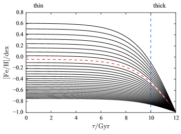
In this section we specify a functional form for the metallicity of the ISM . Fig. 6 of SB09 shows the evolution of in the ISM at a grid of radii. The models of SB09 include full chemical evolution as well as gas accretion and flows. However, despite the complexity of the input model, the resulting form for the ISM metallicity as a function of radius and time is remarkably simple. We find that this evolution can be quite well fitted by the functional form
| (1) |
where and are, respectively, the age and the metallicity of the oldest stars. Hence, like SB09, we assume that the protogalactic material was pre-enriched to some small metallicity . The parameter controls the rate at which metallicity increased at early times, when and . The ratio is large enough that the tanh function is essentially unity for recently-born stars (), so . Hence the function describes the metallicity of the ISM at the current time.
We adopt a current metallicity-radius relation
| (2) |
where is a new constant. Near the Sun the argument of the exponential is small so . It follows that is the current metallicity gradient within the ISM at the Sun, and is negative. At large radii the argument of the exponential becomes large and negative so the metallicity tends to at all radii. Note that when we have set , and the highest metallicity in the disc is set as . Also, in this model the ISM radial metallicity gradient becomes steeper with time.
Fig. 1 shows metallicity against age for a series of birth radii for the choice of parameters that will emerge in Section 5. This plot may be compared with Fig. 6 of SB09. In the SB09 model the radial metallicity gradient is steeper than in most competing models (e.g. Wang & Zhao, 2013; Minchev et al., 2014). Note that this gradient was not fitted to the GCS data by SB09, but instead comes from a fit to open cluster data.
 |
2.2 Quasi-isothermal distribution function
We start from the df of the disc introduced by B12. Its fundamental building block is the quasi-isothermal df:
| (3) |
Each quasi-isothermal is controlled by four parameters, , to be introduced later. Here , and are the circular, radial and vertical frequencies of the circular orbit of radius . We choose positive Galactocentric radial velocity, , to be away from the Galactic Centre and positive azimuthal velocity, , and hence positive angular momentum, , to be in the direction of Galactic rotation. With this convention form a left-handed coordinate system. The factor containing tanh eliminates retrograde orbits (negative ) with the constant . The extent of random motions is controlled by the velocity-dispersion functions
| (4) |
where is a parameter that sets the scale of the outward decline in velocity dispersion within the disc. Numerically, is nearly equal to the dispersion of near the Sun.
The actions given are found using the axisymmetric “Stäckel fudge” algorithm presented in Binney (2012a) with an adaptive choice of the coordinate system parameter, , using the procedure described in the appendix of Binney (2014). Note that as the the potential is axisymmetric is the -component of the angular momentum.
2.3 Galactic potential
Throughout the paper we use an adjusted version of Potential II from Dehnen & Binney (1998) that consists of a thin and thick disc, a gas disc and two spheroids representing the bulge and the halo. This potential is purely axisymmetric and as such does not fully model the central bar of the Galaxy. We have increased the scale-height of the thin disc to and increased the mass of the thin disc such that the circular velocity at the solar radius () is . The functional form for the discs is given by
| (5) |
where is the scale-length, the scale-height, is the central surface density and controls the size of the hole at the centre of the disc which is only non-zero for the gas disc. The spheroids obey the functional form
| (6) |
where . is the scale density, a scale-length, a flattening, and control the inner and outer slopes, and is a truncation radius. The adopted parameters are given in Table LABEL:PotentialParams.
| Thin | / | |
| / | ||
| / | ||
| Thick | / | |
| / | ||
| / | ||
| Gas | / | |
| / | ||
| / | ||
| / | ||
| Bulge | / | |
| / | ||
| / | ||
| Halo | / | |
| / | ||
| / |
2.4 Thin-thick disc decomposition
In the B12 models the disc’s df is a sum of contributions from the thin and thick discs
| (7) |
and the df of each sub-disc is a sum over coeval cohorts, each cohort having a quasi-isothermal df:
| (8) |
The star-formation rates, , are given by
| (9) |
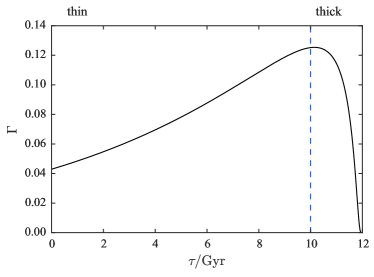
Thus all stars formed prior to are thick-disc stars and all younger stars are thin-disc stars. The global star-formation rate is given by
| (10) |
where is a normalization constant that must be found numerically and . The form of the distribution was chosen such that the star-formation rate increases from zero at the birth of the Galaxy to a maximum at and decays exponentially until the current time. Motivated by the results of Aumer & Binney (2009) we set and leave as a free parameter that controls the thin-thick disc ratio. Fig. 2 shows the form of for the parameters chosen in Section 6.
As in B12 the velocity-dispersion parameters of the thick disc are independent of age. Hence the age of a thick-disc star affects its chemistry but not its kinematics. The parameters of the thin disc depend on age according to the prescription
| (11) |
We model the stochastic heating of the thin disc by setting and , and set .
Now that we have defined the metallicity of the ISM as a function of radius and age, and the dfs as functions of age, we can write a preliminary edf:
| (12) |
This equation states that all stars were born cold in the disc at some radius with some metallicity , which together define a unique age. The stars then heat over time, but their guiding radii remain fixed.
2.5 Radial migration
We now introduce changes in the angular momenta of stars. At a corotation resonance with some non-axisymmetric feature, be it a molecular cloud, a spiral arm or a bar, temporary trapping of a star by the resonance can cause an abrupt shift in angular momentum while leaving the star’s other two actions, and unchanged. Sellwood & Binney (2002) named this process “churning” and argued that such angular-momentum changes from at birth to now bring to the solar neighbourhood metal-rich stars born in the inner Galaxy and metal-poor stars born in the outer Galaxy.
Churning is just one aspect of the diffusion of stars through action space – diffusion parallel to the axis, whereas heating arises from diffusion perpendicular to this axis. Consequently, the proper procedure for constructing an edf is to assume a form for the df of each coeval cohort at birth (e.g. a cold exponential disc as in SB09), and to convolve these with the Green’s function that solves the action-space diffusion equation, (e.g. Binney & Tremaine, 2008, §7.4.2(c))
| (13) |
for a delta-function source of stars at a time in the past. Here is a vector of first-order diffusion coefficients and is a symmetric matrix of second-order diffusion coefficients. That is, we ought to write the general solution to the diffusion equation in the form
| (14) |
where is the probability that a star of age has scattered from to since its birth, and is the df at birth of the cohort of age . is the solution of equation (13) that tends to as .
The orbit-averaged Fokker-Planck equation (13) differs from the standard heat conduction equation by the presence on the right of the term . This term causes a systematic drift towards the origin of action space that counteracts the tendency of the term containing to cause stars to diffuse to large actions, and therefore large energy. In the familiar context of cluster dynamics, the term with describes dynamical friction, while that with drives evaporation.
To the extent to which we can neglect the participation of gas and the dark halo in spiral structure, radial migration should conserve the total angular momentum of the stellar disc. This being so, the tendency of the term in to drive stars to large needs to be counteracted by a term in generating a drift back to .
In the interests of computational speed, we eliminate the integrals in equation (14) over and by guessing that their effect can be approximated by the increases in the velocity-dispersion parameters given by equation (11). We do however evaluate the integral over with equation (13) simplified to
| (15) |
Here we have assumed that is independent of and parametrized it in a form that implies a random walk in with constant steps. If were to vanish, an initial distribution in would remain Gaussian as stars diffused through action space, with the dispersion evolving in time according to
| (16) |
The Green’s function for equation (15) is
| (17) |
Evolving a -function with this Green’s function produces a Gaussian packet that broadens according to equation (16) and drifts in the negative direction with ‘velocity’ .
We relate the first-order diffusion coefficient to our chosen form of by requiring that the df of the whole Galactic disc is a stationary solution of the Fokker-Planck equation (equation 15). In this way the disc does not broaden in time; hence, the total angular momentum is conserved. For simplicity we model our full df by a cold exponential disc in radius with scale-length in a potential with constant circular speed : . The diffusive flux (given by the right-hand bracket in equation 15) vanishes for the stationary df provided
| (18) |
The Green’s function (17) ensures that the disc’s total angular momentum is constant providing the disc is exponential and has a flat circular-speed curve. SB09 enforced conservation of by making the transition probability between grid points in angular momentum depend upon the product of the masses associated with those grid points. Unfortunately, this enforcement makes depend upon , or stated differently, destroys the linearity of the diffusion equation by making the diffusion coefficients functions of the df. Our formalism makes the diffusion coefficients depend on but only for the specific case that is exponential, whilst the SB09 formalism conserves angular momentum for a general . We do not wish to be so sophisticated in this introduction to the edf, but our simple prescription should capture the relevant global properties of radial migration. Recently, Kubryk et al. (2014) have shown that the churning resulting from an -body simulation can be well fitted by a random walk with a spatially varying dispersion, and that the resulting spatial profiles for stars born at given radii match the SB09 results well. It is clear that whilst an individual radial migration event may be awkward to model and depend on the exact form of the scattering potential, a global picture of radial migration can be formed through simple ‘recipes’. The recipe we have presented is perhaps oversimplified but we will show it goes a long way to accounting for the data.
Note that if each population is born as a -function in and and an exponential in such that
| (19) |
and the Green’s function is
| (20) |
then we can perform the integrals over and using the -functions, and the resulting distribution function for the population of age is the one given in equation (21). Thus under highly plausible conditions our prescription for evolving the df of a population by increasing the dispersion parameters and convolving with the one-dimensional Green’s function (17) is equivalent to convolving with the full three-dimensional Green’s function.
2.6 Extended distribution function
With our churning prescription included, the edf becomes
| (21) |
where , . Stars are unable to migrate through so we have included a normalization factor given by
| (22) |
which ensures as shown in Appendix A. Here we introduce the notation
| (23) |
to simplify future expressions.
In Fig. 3 we show the angular momentum distribution of stars born at different radii after they have migrated for using the parameters of our chosen edf given in Section 6. For simplicity we use the thin disc scale-length in equation (18) for . After the main feature is the broadening of the distribution but on longer timescales we observe more noticeably the drift towards the origin. Additionally, we have plotted the exponential disc profile, and we see that by the distributions of the stars born innermost are tending towards the exponential. In Section 6 we will see that our prescription preserves the radial profile of our discs.
The middle and right panels of Fig. 3 make it clear the extent of radial migration that is required to account for the observed breadth of the metallicity distribution in the solar neighbourhood. In particular, stars that are only old and were formed at have a non-negligible chance to be found in the solar neighbourhood. Recently Kordopatis et al. (2015) argued that the metallicity distribution of RAVE stars requires radial migration on this, perhaps surprising, scale.
 |
The approach we have taken lacks a degree of elegance because we have treated radial migration and heating differently, whereas they are in reality just two aspects of diffusion in phase space. Specifically, following B12 we have built heating (diffusion in the and directions) into the basic df, while radial migration (diffusion in the direction) has been explicitly included. This artificial break in symmetry leads to ambiguity as to the value of at which the velocity-dispersion parameters and should be evaluated. If evaluated at the birth angular momentum , this would imply that the star spent its entire life near its radius of birth, while if evaluated at its final angular momentum this would imply that it spent its entire life near its present guiding radius. In reality, the actions and that a star acquires reflect the intensity of the fluctuations in the gravitational field that it has experienced over its entire life, and this intensity will be characteristic of an angular momentum that is intermediate between and .
For a particle undergoing a random walk, the most probable path between and is linear such that, on average, a star at the Sun has experienced the mean of the heating events at the angular momentum passed through. We could therefore opt to evaluate the dispersion parameters at the average of birth and current angular momentum. However, we choose, for simplicity, to evaluate these parameters at the current angular momentum. Experiments using the average angular momentum produce very similar results mostly because the best-fitting scale-lengths for the velocity dispersions are large so the dispersion parameters don’t vary significantly with radius.
Indeed, Minchev et al. (2012) showed from a numerical simulation that the final velocity dispersions of stars that had migrated into a given radial bin matched the final velocity dispersions of stars that had spent their entire lives in that bin. Kordopatis et al. (2015) have found that an analogous result holds for stars sampled by the Radial Velocity Experiment (RAVE). This gives us confidence that our approximation is a valid one.
2.7 Performing the integrals
To evaluate equation (21), we need to evaluate a double integral over and . Fortunately, one of these integrals is trivial as the integrand contains a -function. When we use the -function to evaluate the integral, we obtain derivatives of with respect to either or in the denominator of the integrand. The choice of whether to perform the or integral first depends upon the properties of these derivatives over the integration range. We note that , and . Therefore, for the thin disc we use the -function to perform the integral and for the thick disc we use it to perform the integral. For the thin disc, we obtain
| (24) |
where is given by , which may be inverted analytically. Additionally, we have that
| (25) |
For the thick disc, we have
| (26) |
where
| (27) |
Again we find by inverting analytically. For convenience, we limit the integration range to and perform the integral over . These two one-dimensional integrals are then performed numerically using a 10-point Gaussian quadrature scheme.
2.8 Halo edf
One practical problem with the above edf is that any star that falls outside the allowed range in (e.g. ) is deemed unphysical by the model (assuming negligible errors in the metallicity). This problem can be solved by the inclusion of a df for the stellar halo. The data to which we will fit the edf are not very sensitive to the stellar halo, but the inclusion of a halo df allows us to assign any ‘unphysical’ star to the halo.
We construct a simple action-based distribution function for the halo of the form (Posti et al., 2015)
| (28) |
The model generated by this df has a simple power-law density profile with a core that is specified by the parameter . We choose . This model has a density profile outside its scale radius of , and inside, and has velocity dispersions at the Sun of (Brown et al., 2010). The factors multiplying and are approximately and at the solar position such that the halo model is approximately isotropic. In addition to this action-based part, we include a simple Gaussian in metallicity such that our halo edf is given by
| (29) |
We set the mean metallicity as and the width of the metallicity distribution function as . We assume all stars in the halo are of age . In what follows, the weight of the halo, , is allowed to vary, but we expect that it will be such that the halo contributes in the solar neighbourhood (Jurić et al., 2008).
3 Data
Here we introduce the data to which we will fit edfs and with which we will then test its predictions. We require seven-dimensional data (six phase-space coordinates and the metallicity ). We use data from the GCS and SEGUE survey, complemented by the stellar density data from Gilmore & Reid (1983). Additionally, we place the Sun at and (Binney et al., 1997) and we use the peculiar solar velocity from Schönrich, Binney, & Dehnen (2010): (recall positive is away from the Galactic centre and positive is in the direction of Galactic rotation such that form a left-handed coordinate system).
3.1 Geneva-Copenhagen Survey
The Geneva-Copenhagen Survey (GCS) (Nordström et al. 2004; Holmberg et al. 2009) is a sample of nearby F and G stars extending out to . Through a combination of photometry, line-of-sight velocity, Hipparcos parallax and proper motion observations, the catalogue provides a view of the chemo-dynamical structure of the solar neighbourhood. We use the most recent re-analysis of the survey by Casagrande et al. (2011). These authors used the infrared flux method (IRFM) to produce more consistent effective temperature and metallicity scales. This re-analysis found that the stars were on average more metal rich than in previous analyses. We use all stars in the catalogue with proper motions that were flagged by Casagrande et al. (2011) as having reliable metallicity determinations. This reduces the data set to stars.
Because the GCS is a local survey, it is dominated by thin-disc stars, and the influence of the thick disc is subtle (Binney, 2012a). Due to the accuracy of the Hipparcos astrometry, the GCS provides us with a precision velocity distribution in the solar neighbourhood, and led to the discovery of substructures in the plane (Dehnen, 1998). In particular, the peak of the distribution is associated with the Hyades moving group, and the Hyades and Sirius moving groups endow the distribution with a flat top. The distribution appears free of substructure (Dehnen, 1998). The presence of substructure is important when attempting to fit a zeroth-order model as it makes the comparison of model and data more difficult to interpret.
The data we use for each star are , along with the corresponding errors, where is the parallax, is proper motion and the other symbols have their usual meanings. We adopt the reported errors in , and following Casagrande et al. (2011) we use for all stars.
3.2 SEGUE G dwarfs
The Sloan Extension for Galactic Understanding and Exploration (SEGUE Yanny et al., 2009) is a low-resolution spectroscopic survey of stars fainter than , complemented by photometry. As such, it provides a view of the outer parts of the disc, dominated by the thick disc, and the stellar halo of the Galaxy, and so complements the more local GCS sample. The SEGUE data are available as part of SDSS DR10 (Ahn et al., 2014). These data were reduced using an improved SEGUE Stellar Parameter Pipeline (SSPP) (Smolinski et al., 2011), which, like the latest GCS re-analysis, used the IRFM to produce more consistent effective temperatures. However, this did not significantly affect the obtained metallicities.
Here we use only SEGUE data that satisfy the target selection criteria for G dwarfs: a star with and . From the G dwarfs, stars were selected that (i) have to ensure completeness at the bright end, (ii) are given valid parameter estimates by the SSPP, and (iii) were not flagged as noisy or with a temperature mismatch. In addition, we impose a cut in surface gravity, , to ensure we include only dwarf stars, we remove both stars with SNR and stars in fields with on the Schlegel et al. (1998) extinction maps. Finally we remove stars with no measured line-of-sight velocity or proper motions. The final sample contains stars.
We estimate the distances to SEGUE stars using the method presented in Schlesinger et al. (2012). The majority of the stars are from the outer disc, so we expect them to be old. We, therefore, assume all stars have an age of . Using the YREC isochrone provided by An et al. (2009), we first bracket the provided metallicity for each star with two isochrones. For each isochrone, we find the closest entry to the star’s reported colour. The magnitudes are found by linearly interpolating between the two entries in each isochrone. The distance is determined by averaging the five estimates from each of the extinction-corrected bands. We make no consideration of the errors in the colours, magnitudes and metallicities. A Bayesian distance-estimation algorithm, such as that presented by Burnett & Binney (2010), would be preferable. However, for dwarf stars, we expect the cruder approach of Schlesinger et al. (2012) to be adequate – they estimate the errors in their distances and conclude that there is a random distance uncertainty of for stars with , and for more metal-poor stars, in part due to errors in the isochrones. Additionally, there are systematic distance uncertainties arising from the single-age assumption (expected to produce a distance overestimate for the metal-rich stars) and the presence of undetected binaries produces a distance underestimate for approximately of the population. In what follows we neglect both of these systematic errors.
3.3 Gilmore-Reid density curve
Gilmore & Reid (1983) measured the stellar density as a function of distance away from the Galactic plane, by observing a sample of K dwarfs towards the South Galactic Pole. This was the first study to indicate the existence of a thick disc.
4 Selection functions
Before comparing our model to data, we must understand the selection effects of a survey. In this section we discuss (i) how we include the selection function in our modelling approach, (ii) the selection functions for the GCS and the SEGUE survey, and (iii) the possibility of avoiding explicit use of a selection function.
The selection function of a survey is the probability of a star being in the catalogue given its properties. The selection is nearly always done on the basis of the observed properties of a star. If we denote as meaning ‘in the survey’, the probability of an individual stellar datum, , given the model, , and given it is in the survey, , is
| (30) |
where we call the selection function, the distribution function, and is the probability that a randomly chosen star in the Galaxy enters the catalogue given a particular model. only comes into play when fitting the model to the data.
Stars are selected for inclusion in a spectroscopic survey, such as SEGUE, from a photometric survey on the basis of criteria involving apparent magnitude and possibly colour. To relate colours and magnitudes to the physical properties of stars such as age and metallicity, we require a set of isochrones. We use BaSTI isochrones (Pietrinferni et al., 2004) spaced by for and for for each of the metallicities listed in Table 2. We assume that all populations of fixed metallicity and age were born with a universal initial mass function (IMF), . We adopt the Kroupa et al. (1993) IMF
| (31) |
Here is the mass of the star in units of the solar mass. With this choice, we can write down our full distribution function as
| (32) |
| Z | Y | |
|---|---|---|
| 0.00001 | 0.245 | -3.27 |
| 0.0001 | 0.245 | -2.27 |
| 0.0003 | 0.245 | -1.79 |
| 0.0006 | 0.246 | -1.49 |
| 0.001 | 0.246 | -1.27 |
| 0.002 | 0.248 | -0.96 |
| 0.004 | 0.251 | -0.66 |
| 0.008 | 0.256 | -0.35 |
| 0.01 | 0.259 | -0.25 |
| 0.0198 | 0.2734 | 0.06 |
| 0.03 | 0.288 | 0.26 |
| 0.04 | 0.303 | 0.40 |
Below we assume that the selection functions involve apparent magnitude, colour, and . A combination of , and taken with the isochrones uniquely determine a colour and an absolute magnitude. Coupled with a distance, the absolute magnitude implies an apparent magnitude. Therefore, we can consider a selection in colour and magnitude as a selection in mass, metallicity, age and distance.
If we want to determine the distribution of the arguments of our distribution function, , with a selection of this form, we write
| (33) |
where
| (34) |
can be calculated independently of the dynamical model. In particular, if the selection function is independent of and we must only engage with the isochrones once. The resulting pre-tabulation can then be interpolated for any choice of ; any call outside the grid uses the nearest grid point.
4.1 GCS selection function
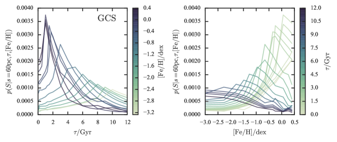
For the GCS, we use the selection function in SB09, which was approximately constructed using the selection rules from Nordström et al. (2004) and comparison with the target catalogues. The result is a simple selection function in Strömgren colour and apparent magnitude, . We assume that the selection function is independent of the line-of-sight such that . Following SB09, we first cut the isochrones at the bottom of the red giant branch (flagged in each isochrone and corresponds to a minimum in the luminosity for high-mass stars). This cut fails to remove many model stars that lie on the subgiant branch of an isochrone, and the GCS does not include such objects. Therefore, we also cut all isochrone points with and to reproduce approximately the edge of the sample observed by Casagrande et al. (2011)111Importantly and .. For each isochrone, we form a grid in the logarithm of distance between a minimum value and the value at which the selection function falls to zero. At each distance , we find for each isochrone. Thus, we construct a three-dimensional grid over which we can interpolate given any triple . Fig. 4 shows the resulting selection function for a star located at (approximately the peak of the GCS distance distribution). We see that it peaks at around , where the majority of GCS stars lie (Casagrande et al., 2011).
 |
4.2 SEGUE selection function
In Bovy et al. (2012c), it is shown that the SEGUE G dwarf selection is uniform in and a near step function in . The position of this step depends upon the plate , in particular whether it is a bright or faint plate, and has the functional form
| (35) |
where depends upon the plate, and is the fraction of SDSS targets that have spectra. The selection function is set to zero outside the magnitude interval for bright plates and for faint plates. Additionally we set the selection function to zero for . We use the publicly available code from Bovy et al. (2012c) to find the location of for each plate by comparison with SDSS. Note here that, unlike the GCS, the selection function depends upon the line-of-sight and as the selection function depends upon the plate . In Fig. 5, we show the selection function for a star at observed in the faint plate #. We see that it is approximately flat with age and falls to zero for . Even without a physically-motivated model, i.e. one in which the stars at high altitude are metal-poor, the SEGUE selection function for the faint plates is such that metal-poor stars are preferentially selected. However, the selection function for the bright plates includes many metal-rich stars.
 |
4.3 Side-stepping the selection function
We have just detailed appropriate selection functions for the GCS and the SEGUE G dwarf sample. However, sometimes the selection function of a survey is either overly complex or hard to determine because it depends on possibly un-documented historical and social factors – particular objects might have been added to the target list because they were suspected of some special property, while other objects fall away on account of unusual difficulties. This is very likely to be the case when a survey is still underway. In these cases, it may be difficult to construct the selection function accurately. Here we discuss how a model may be compared to data without reference to the selection function.
Say, from a survey, we have for each star all the observables in the set . If we know that the survey is constructed by selecting on a subset of these observables, denoted , then there is a subset of observables on which there has been no explicit selection. For instance, we may know that the selection was performed in colour but not in velocity. Therefore, the velocities are free from an explicit selection although they are implicitly biased by the selection since any relation between velocity and colour, e.g. bluer stars are younger and so have a lower velocity dispersion, implies that selecting blue stars lowers the velocity dispersion of the sample.
In this case, we proceed by considering the conditional probability . We write
| (36) |
We know that the selection is only in the observables so . Therefore, we find that
| (37) |
This equation states that the conditional probability of the observables given the other observables and the fact this star is in the sample is just the conditional probability of the observables given the other observables regardless of how the selection on is made. All we need to know is that we have selected only on .
This argument underpins models of the disc obtained from velocity histograms (Binney, 2012a; Binney et al., 2014). For a survey such as RAVE, the selection is not performed on the line-of-sight velocities or proper motions. Therefore, given a set of observables for each star, we can sample a set of velocities from the model. These velocities may then be used to construct histograms to compare with the data. The approach taken by Piffl et al. (2014) was first to bin the data in and then to sample the distribution in at the centroid of each bin. For this approach, we should dissect the sample into small cells in -space because without the selection function we do not know with what weights the should be added to form the sample-wide distribution . Finally, we note that for the above approach to be mathematically valid, must contain all observables used in the selection. The approaches of Binney et al. (2014) and Piffl et al. (2014) did not use the apparent magnitude information of each star. Additionally, Piffl et al. (2014) select a giant subsample of the RAVE survey using . Therefore, to use the above approach on this subsample we have . By neglecting to use and instead using the distance, we have implicitly biased the age distribution of the stars and hence the velocity distributions.
The disadvantage of this route around the problem of the selection function is that we end up not using the available information to the full. Consider, for instance, the case of the RAVE velocity sampling. With a full dynamical distribution function, the power comes from the link between the spatial and velocity distributions, which are connected by the potential. For a fixed potential, we may be able to find a velocity distribution that matches the data, but the spatial distribution will then match the data only if we have found the true potential. This is the principle that was used by Piffl et al. (2014) to constrain the distribution of dark matter. If we consider only velocity information, we lose this power and can only rely on spatial gradients in the velocity distribution for any constraint. To constrain the potential, one must engage with the selection function of some survey, which Piffl et al. (2014) implicitly did by adopting the vertical density profiles of Gilmore & Reid (1983) or Jurić et al. (2008).
The second problem with the above approach is that it is more expensive computationally than an approach that uses the selection function. If we use equation (30) to fit the data, we must calculate the denominator once to sufficient precision that, the error in the th power of (where is the number of data points) does not dominate our posterior probability (McMillan & Binney, 2013). However, this is a single computation for each considered model. When we do not explicitly use the selection function, as in equation (37), we must compute the denominator for each star to comparable precision. One way of approaching this is to tabulate the integral on a grid in and interpolate. However, the dimensionality of can be large, and it is challenging to reduce interpolation errors such that the noise does not dominate the posterior probability.
In conclusion, one can model a survey without knowing the selection function, but at increased computational cost and giving reduced diagnostic power for a given model than when the selection function is used. However, in certain cases one may have no choice but to proceed without the selection function. In the following, we do use selection functions.
5 Choice of parameters
We now turn to fitting our edf to data. To choose the parameters of our model, we use the GCS and Gilmore-Reid data, and vary the parameters:
We seek to maximise given by
| (38) |
where
| (39) |
where is a 5D Gaussian to give the convolution of the observables with the errors and the primed quantities are functions of . is the selection function as detailed in Section 4.1. This approach uses uniform priors on all model parameters. However, we note that our results are essentially independent of our choice of weak prior on the model parameters. We perform the integral over the errors () using Monte Carlo integration. Following McMillan & Binney (2013) we use a fixed sampling of points per star to remove numerical noise and to allow pre-computation of the actions: if we were to draw new Monte Carlo sampling points for each set of parameters in the edf, our parameter choices would be dominated by numerical noise.
We assume that the completeness along each line-of-sight is the same such that
| (40) |
We perform this integral using the Vegas algorithm implemented in the cuba package Hahn (2005).
We also use the Gilmore-Reid data in the fits. The log-likelihood of the Gilmore-Reid data is given by
| (41) |
where is the density profile from Gilmore & Reid (1983), are the errors in and is the density profile calculated using the edf integrated over all metallicities. The quantity we seek to maximise is
| (42) |
We perform this procedure using the Nelder-Mead multi-dimensional minimization routine (Nelder & Mead, 1965) implemented in the Gnu Science Library (Galassi et al., 2009). is some weight which we set to . This is to encourage the fitting procedure to take the rather few Gilmore-Reid data points seriously. The introduction of can be considered as a restrictive prior on the density of the models considered in fitting the GCS. Additionally, it dilutes the effects of substructure in the GCS, which we do not want to fit.
6 Results
The parameters selected by the Nelder-Mead algorithm are given in Table 3. We note that whilst our procedure is statistically sound, we know the model will not perfectly match the data because (i) we are using a fixed potential, (ii) our model ignores substructure like that seen in the GCS velocity distribution, and (iii) the Nelder-Mead algorithm is likely to select a local minimum, particularly for high-dimensional problems.
6.1 MCMC exploration of model space
In addition to the minimization routine, we have also performed a fuller MCMC search of the parameter space. The parameters chosen by the Nelder-Mead simplex algorithm lie within two standard deviations of the centres of the one-dimensional posterior distributions from the MCMC chains.
As expected from a very local sample, the scale-lengths of the discs are not well constrained by the GCS data. The thin disc velocity-dispersion parameters are, by contrast, constrained to less than . Similarly, the thick disc radial velocity-dispersion parameter is constrained to about , whilst the vertical velocity-dispersion parameter is anti-correlated with the weight of the halo and so not as well constrained. Additionally, the current ISM gradient parameter is constrained to so that at the Sun the ISM metallicity gradient is . This agrees remarkably well with the radial metallicity gradient for Cepheids from Genovali et al. (2014) (). The radial migration parameter is such that the oldest stars have migrated during the lifetime of the Galaxy, but much higher migration strengths () are also compatible with the data. One might anticipate, however, that the data might be consistent with lower radial migration strength and steeper metallicity gradient, which interestingly is not favoured by the model. It appears that the youngest stars constrain the local metallicity gradient whilst the width of the metallicity distribution constrains the degree of radial migration required. As we have only explored a single ISM metallicity parametrization the tight constraint on the local metallicity gradient may be a result of our tight parametrization and other variations of the metallicity with time could be explored. For instance one of the Chiappini et al. (2001) models produces a shallowing metallicity gradient with time at late times which is not a possibility with our parametrization.
| Thick | Thick disc scale-length | ||
|---|---|---|---|
| Thick disc velocity-dispersion scale-length | |||
| Thick disc radial velocity-dispersion parameter | |||
| Thick disc vertical velocity-dispersion parameter | |||
| Thin | Thin disc scale-length | ||
| Thin disc velocity-dispersion scale-length | |||
| Thin disc radial velocity-dispersion parameter | |||
| Thin disc vertical velocity-dispersion parameter | |||
| Other | ISM radial metallicity gradient at solar radius | ||
| ISM metallicity at birth of Galaxy | |||
| Early star formation growth timescale | |||
| Radial migration strength | |||
| ISM metallicity enrichment timescale | |||
| Radius of current ISM solar metallicity | |||
| Stellar halo weight | |||
| Not fitted | Thin disc radial heating growth parameter | ||
| Thin disc vertical heating growth parameter | |||
| Age of Galaxy | |||
| Age of thin-thick disc separation | |||
| Thin disc star-formation rate decay constant | |||
| Parameter to control velocity dispersions of stars born today | |||
| Mean metallicity of stellar halo | |||
| Width of metallicity distribution of stellar halo |

We will not report further on the results of the MCMC searches of parameter space because we have only varied the parameters of the edf, and not the parameters of the potential; we defer a full fitting procedure (including the potential) to a future paper. Since we are not fitting the potential, we cannot hope to obtain a statistically optimal representation of the data. Rather we seek a good model. Below we examine how well the data are fitted by the model chosen by the Nelder-Mead simplex algorithm as described in Section 5.
6.2 The best-fitting model
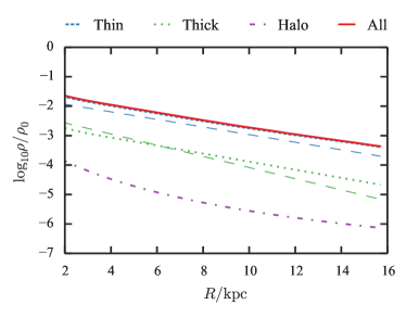
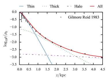
We begin by inspecting the global properties of the model. Fig. 6 shows the global radial and vertical profiles of the full model and of the individual components. Along with the radial profiles we have plotted the profiles of the discs at their birth and we see that our radial migration prescription has preserved the radial disc profiles. The thick disc profile is slightly broadened as we are using the thin disc scale-length to calculate . In the vertical density panel we also show the Gilmore & Reid (1983) data which are well fitted by our edf.
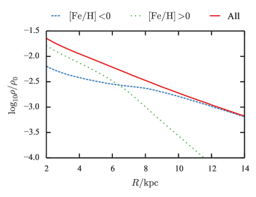
In Fig. 7 we plot the radial density profiles for different sub-populations. In the left panel we show the radial density profiles for super-solar and sub-solar metallicity populations. We observe that the total profile is exponential whereas neither sub-population can be well modelled by a single exponential. This finding contrasts with the contention of Bovy et al. (2012c) that all mono-abundance populations have exponential density profiles. In the right panel of Fig. 7 we show a further subdivision into four bins: the thin disc with and with , and the thick disc with and . If we fit an exponential to the density profiles of these structures in the solar neighbourhood, we find local scale-lengths of () for the thin disc metal-poorer (richer) than , and () for the thick disc metal-poorer (richer) than . We obtain a very long scale-length for the low-metallicity thin-disc population because its profile is not really an exponential. The analysis of the SEGUE G dwarf data in Bovy et al. (2012c) produced a similar result.
6.2.1 Sampling mock catalogues
To compare our model and data, we sample mock catalogues from the model. At the reported and of each star in a catalogue we sample distance, metallicity and velocity. We use a simple rejection-sampling technique using a uniform distribution in distance and Gaussians in metallicity and Galactocentric velocities. We sample from the distributions (where denotes the datum and the survey), convert the quantities to Galactic coordinates and scatter by the reported error in the datum. For this procedure to be valid, we require the errors in the observables to be independent of , , , and . In the histograms that follow, the errorbars show the Poisson error and do not give any indication of the size of systematic errors in the models. We use black points for the data, and coloured points for mock catalogues drawn from the edf.
6.2.2 Apparent magnitude cut
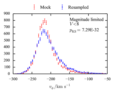
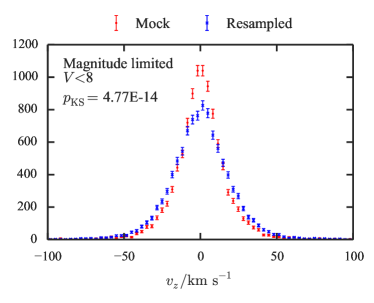
Before comparing to actual data, we perform a simple experiment to demonstrate the importance of selection functions and of adding metallicity information to the df. We construct a sample of stars along the line-of-sight , with the selection function
| (43) |
which creates a magnitude-limited sample. We note that our sample will not contain any stars with as the BaSTI isochrones do not contain any points with . Approximately of the stars in our sample have , so we anticipate that there should be fewer than stars in our sample with . This small number should not affect the statistics. The resulting mock metallicity and velocity distributions are shown in red in Fig. 8. We now turn the selection function off (set ) and resample the velocities given , , distance and metallicity. The blue points in Fig. 8 show the resulting distributions. If there were no correlations between the kinematic and intrinsic properties of stars, the velocity distributions of the two mock catalogues would be identical. However, the stars of a young cohort are on average more luminous than the stars of an older cohort, and consequently the proportion of younger stars in a survey is greater than the proportion of these stars at any location in the Galaxy. Since young stars tend to have smaller random velocities than old stars, an observational sample has smaller velocity dispersions than all the stars at a given location. When we turn off the selection function, we are not biased in age and we obtain broader velocity distributions that reflect the underlying distributions. The Kolmogorov-Smirnov probabilities, , that the red and blue samples in Fig. 8 are drawn from the same distribution are .
We performed this experiment with a fainter cut, , and found that the difference between the two velocity distributions was reduced. Adopting this fainter cut decreases the relative proportion of nearby young stars and increases the proportion of distant old stars. Consequently, the resulting sample is more representative of the underlying population in all respects, including its velocity distributions.


The selection function used in this experiment is simpler than the selection function of a real survey but it serves to show the importance of grappling with the selection function. Given the dependence of luminosity and colour on metallicity, this requirement obliges us to work with edfs rather than dfs.
6.2.3 GCS mock catalogue
We now build a mock GCS by sampling our model by the technique described at the start of Section 6.2.1 using the selection function given in Section 4.1. The sampling neglects any correlation between the errors and distance, metallicity or velocity. In the GCS the most prominent correlation is that between the parallax error and the magnitude (Pearson correlation coefficient between and ). However, the parallax error does not correlate as well with the parallax (Pearson correlation coefficient between and ), so we neglect this effect and simply use the reported parallax errors for each star.
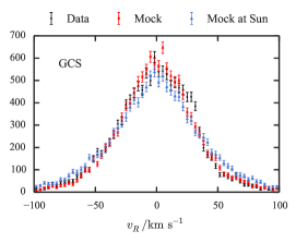

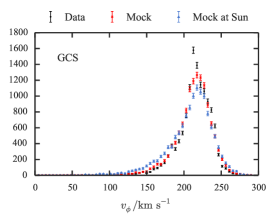
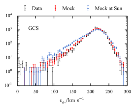
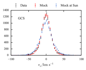


 |
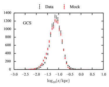
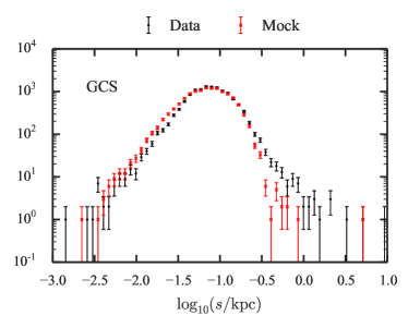
Fig. 9 shows the distance distributions of the data (black points) and the mock sample. The peaks of the model and data distributions match well but the mock sample is slightly skewed with respect to the data sample in the sense that the latter has too few distant stars and too many close stars. This potentially indicates that the selection function is sub-optimal. We have assumed that the angular selection is isotropic which may bias the distance distribution slightly. Note, additionally, we anticipate that the nearer stars will have, on average, been assigned higher distance errors than expected, whilst the more distant stars will have been assigned smaller distance errors. From the correlation coefficients quoted previously, we expect this effect is small. However, it would produce a discrepancy of the type encountered here.
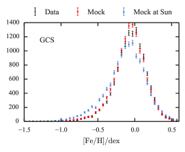
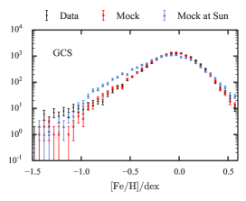
Fig. 10 shows the metallicity and velocity distributions. The model (red points) matches the data (black points) well for . For the model slightly underpredicts the data but the significance of the mis-match is low as there are only a few stars at these low metallicities. The fitting procedure seeks to match the high- points from the Gilmore-Reid data at the expense of underpredicting the number of low-metallicity stars. Clearly this deficiency is due to the simplicity of our halo model. We will see again when inspecting the SEGUE data that our halo model is not optimal.
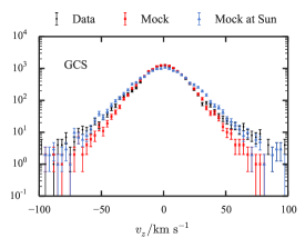
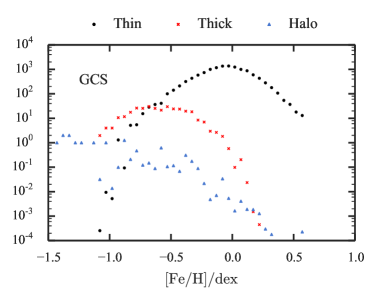
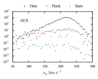
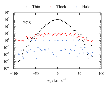
The velocity distributions in Fig. 10 are fitted well by the model (red points), particularly those for and . The model distribution fails to match the peak of the data distribution, but this peak is due to the Hyades stream, a non-equilibrium feature that we are not concerned with matching. Fig. 11 shows the contributions to the mock catalogue from thin-disc, thick-disc and halo stars. We see that, as expected, the thin disc dominates over most of the space explored although the thick disc dominates for and .
In Fig. 10, blue points show a mock catalogue generated by sampling new metallicities and velocities at the solar position with the selection function turned off. If the GCS velocity histograms were fair samples of the local velocity distributions, the blue and red points would agree. Actually the blue velocity histograms are broader than the red ones. Also, the blue metallicity distribution has a broader metal-poor wing. These differences arise because by turning off the selection function, we have increased the number of high-age stars – Fig. 4 shows that the typical age of GCS stars is .
We find the best-fitting vertical velocity-dispersion parameter for the thin disc is . This value is larger than previous values, for example those to derived by B12, because we include the bias in the GCS towards younger stars and report the velocity-dispersion of the underlying thin-disc population.
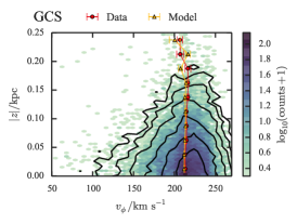
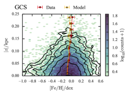
Fig. 12 shows the density of stars in the , and planes. The data and models match well and the red and gold points show that the means of and binned in /metallicity are well recovered.
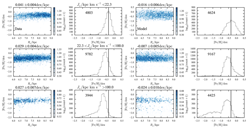
Fig. 13 shows the gradients of the metallicity with respect to the guiding-centre radius and the metallicity distributions in three bins in vertical action . The two columns on the left show data and the two on the right show the mock GCS catalogue. In the two low- bins, the gradient is well recovered. The gradients in the high- bin are more discrepant although consistent within . Additionally, we find that the metallicity distributions for all three action bins are well matched. Note that the peak of the metallicity distribution remains fixed with increasing vertical action for both the data and the model.
6.2.4 SEGUE G-dwarf mock catalogue
We now examine a mock catalogue of SEGUE G dwarfs constructed using the edf of Section 6.2.3 and the selection function of Section 4.2. The comparison of a mock SEGUE catalogue with the real one is a rigorous test of our methodology in two respects. First, the input to the edf from stars further than from the Sun is very small, being restricted to the Gilmore & Reid (1983) density profile. Hence the velocity and metallicity distributions in the mock catalogue are pure predictions and are exposed to inaccuracy of the adopted gravitational potential. Second, the distances used for SEGUE stars are based on a different set of isochrones from those used to derive distances to GCS stars. Any discrepancy between the isochrone sets can be expected to lead to mismatches between the mock and true catalogues.
Our first attempt to make a mock catalogue revealed that the halo weight, , was too large, so we reduced by a factor of 6. The GCS does not constrain the halo tightly, and the strongest constraint on comes from the Gilmore-Reid data. After making this alteration, the densities at high are slightly underestimated. While the degree to which we can trust these high- densities is unclear, it is likely that the need to revise reflects shortcomings in our model. Indeed, the halo edf is intentionally very crude, and there is the suggestion from Binney et al. (2014) that the distribution for the thick disc is not appropriate. Therefore, there is plenty of scope for adjusting the models, and the model we present here is surely sub-optimal.
Fig. 14 shows that there is a small mismatch between the distance distribution of the model (red) and that of the data (black). The model predicts slightly too few nearby stars and too many distant stars. We can understand one potential cause of this trouble by inspecting the metallicity distributions of Fig. 15. The model metallicity distribution peaks in the correct place and has a broad peak approximately the same width as the data peak. We note that the smooth increase in star formation rate at early times produces the rising low-metallicity edge of the distribution. At high metallicities () the model predicts many more stars than are observed. Here we are seeing the thin disc of the model. It is these additional stars that seem to be distorting the distance distribution. At fixed apparent magnitude and colour, increasing the metallicity of a dwarf star shifts it in the HR diagram up from below the solar-metallicity main sequence and thus moves it to a larger distance. We will return to the dominance of the metal-rich population below.

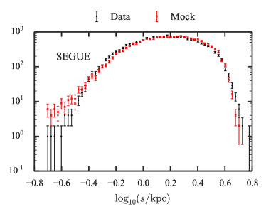
Fig. 15 also shows the velocity distributions of the data and the model. The distribution is a good match though the model is slightly broader than the data for large . This may be due to too much halo contribution (although from inspecting the metallicity distribution it seems our halo weight is approximately correct) or more likely the thick disc velocity dispersion is slightly too large. This second option is corroborated by the distributions. The model fails to match the peak in the data and is broader than the data. Again, judging by the match to the counter-rotating stars it appears our halo weight is correct. Decreasing the velocity-dispersion parameter of the thick disc would underpopulate the wings of the GCS distribution so it seems that the solution is to adjust the potential. We anticipate that at least some parts of our model will be inconsistent with the SEGUE data as we have used a fixed potential. Interestingly the distribution broadly matches the data but the mean of the data is clearly offset from zero. There has been much in the literature recently associating mean vertical velocity shifts with modes in the disc (e.g. Widrow et al., 2012; Williams et al., 2013). However, this shift in the peak could also arise from systematic distance errors or zero-point errors in the SDSS proper motions.

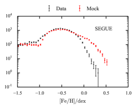
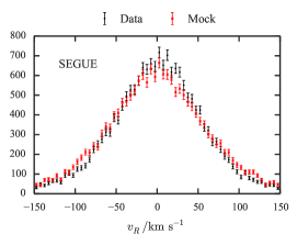
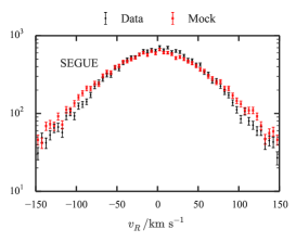
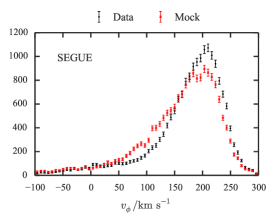
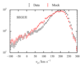


Fig. 16 shows the contributions of the thin and thick discs (black and red) and the halo to the metallicity and velocity distributions. The top left panel clearly shows that the main peak and the high-metallicity wing in the overall metallicity distribution are, respectively, associated with the thick and thin discs. The absence of a high-metallicity wing in the observed metallicity distribution signals that the model exaggerates the contribution of the thin disc to the sample. We require a very dominant thin disc population in the plane to match the GCS data as well as provide a good fit to the Gilmore & Reid (1983) density curve. Additionally our high vertical velocity dispersion for the thin disc implies a larger scale-height such that thin disc stars are dominant up to . However, the SEGUE data require a much smaller thin disc contribution which seems to point towards a smaller thin disc scale-height. However, for this option to then match the Gilmore-Reid density data we would require an adjustment to the potential. The data here are clearly very informative and require a very finely tuned model in order to describe all the features.
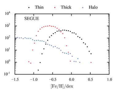
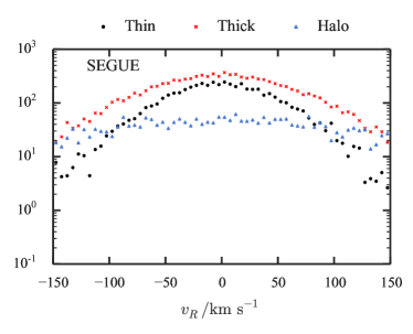
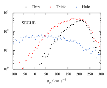
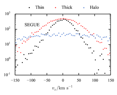
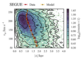
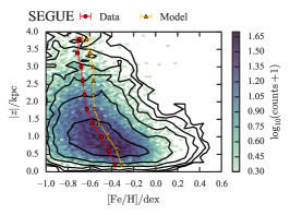
Fig. 17 shows the distribution of stars in the , , and planes – colours show data and contours the model. The contours wrap round the peaks of the data distribution very nicely, but in the central and right panel they extend too far to the right, signifying that the model contains more metal-rich stars than the data.
In each panel the red points show the mean abscissa in the data at the given ordinate, while the gold points show these means in the model. In the left panel we observe that the runs of mean with agree well, suggesting that the potential is close to the truth. On account of the surfeit of metal-rich stars in the model, the model means lie to the right of the data means for the central and right panels. In the central panel, this effect is largest at low and even reverses sign at . The excess metal-rich stars in the model are contributed by the thin disc.
The right-hand panel of Fig. 17 shows that the mean metallicity decreases at the correct rate with throughout the SEGUE volume. However there is a systematic difference of in the mean metallicity. At low this is due to the unwanted presence of the metal-rich thin disc in the model.
In Fig. 18 the first column shows the density of SEGUE stars in the plane with the stars sorted into three bins by . The third column shows the same distributions for the mock catalogue. In each panel the stars cluster into a nearly horizontal band because at any value of the stars are widely distributed in guiding-centre radius . Above each panel we give the slope of the band’s ridge-line found from linear regression. For the data distributions the gradient is positive, whereas it is negative for the top two model panels (lowest values of ) and close to zero in the bottom panel. The positive gradients of the data distributions echo the finding of Lee et al. (2011) that -enhanced stars exhibit a positive gradient of with metallicity.
The second and fourth columns of Fig. 18 show histograms of for each bin in . Our model captures the essential features of the data although with varying degrees of success. The peaks of the data distributions are replicated by the model. At low the model distribution is too wide due to the unwanted contribution of the thick disc. At high the relative thick disc to halo weight is perhaps slightly off or the halo model needs adjusting. In particular, our model produces a small peak at which is the centre of the Gaussian used to model the halo metallicity distribution. The data is unimodal and steadily declines towards low metallicity.

 |
6.2.5 Adjusting the model
Our model has performed surprisingly well in predicting the SEGUE G dwarf data considering we have not adjusted the potential. Here we discuss some attempts made to improve the SEGUE predictions. The most obvious discrepancy between model and data is the over-abundance of metal-rich () stars in the model. We wish to decrease the impact of the thin disc at intermediate Galactic heights whilst retaining a dominant thin disc population in the GCS sample. We tried decreasing by setting and simultaneously decreasing such that the younger populations remained at fixed velocity dispersion whilst the older populations were made cooler and so less dominant with height. However, this did little to reduce the number of metal-rich stars in the SEGUE G dwarf sample. Additionally, we tried increasing to such that the relative number of hot metal-rich thin disc stars from the inner Galaxy was reduced. Again, this did little to remedy the situation. Finally, we tried evaluating the velocity dispersions at the radius of a circular orbit with angular momentum as this location better reflects the disc environment that heats the given star. This would cause the contribution of the thin disc to die off faster with Galactic height as velocity dispersion falls with radius. However, as the scale-lengths of the velocity dispersions are long in our model this small adjustment does not significantly change the predictions.
Another deficiency of the model is the inability to match the trend of with and the model does not produce the positive gradients of seen in Fig. 18. In order to improve the situation we tried breaking the assumption that the thick disc is a single quasi-isothermal and made the scale-length a linear function of age from at the birth of the Galaxy to at . This model assumes the Galaxy formed inside-out. This did not improve the run of with and actually produced more metal-rich thick disc stars in the sample, and thus shifted the model metallicity distribution to higher . One problem is that the strong radial migration broadens the thick disc so the kinematic signal of inside-out formation is washed out and we are left with the chemical signature: a higher abundance of metal-rich stars.
7 Conclusions
We have presented a simple extension of the action-based distribution functions of B12 to include metallicity information. Our model is the first continuous chemo-dynamical model in the literature and is constructed such that the spatial and kinematic distributions are consistent with a realistic Galactic potential. Inspired by the full chemo-dynamical evolution models of SB09, we included analytically the relationship between metallicity and dynamics. The model explicitly includes a simple, but novel, radial migration prescription that causes the solar metallicity distribution to broaden as stars migrate to from the inner and outer disc. Despite the simplicity of our radial migration prescription we have shown that it preserves the radial profile of the disc and hence the total angular momentum of the system.
All surveys have a selection function that restricts apparent magnitude. The luminosity of a star depends on its initial mass, its metallicity and its age according to the appropriate isochrone. By selecting on apparent magnitude, we select on a combination of mass, age and metallicity, and we need an edf to model this selection, as we must before we can properly compare a model to data.
We showed that selecting solar-neighbourhood stars on apparent magnitude alone, implies a strong selection on age. Because young stars have smaller random velocities than old stars, by preferentially selecting young stars, an apparent-magnitude cut returns a sample with a materially smaller velocity dispersion than that of the underlying population. This effect, which makes the GCS stars younger than the local population, has been neglected in recent studies that employed a df, such as B12 and Piffl et al. (2014).
Fortunately, the requirement to use an edf rather than a df is an opportunity as well as a necessity. The opportunity has two parts. First, an edf should to lead to tighter constraints on the Galactic potential because each observationally distinguishable chemical population has its own dynamics yet must be consistent with the same Galactic potential. Walker & Peñarrubia (2011) have demonstrated the value of this principle in the context of two populations within dwarf spheroidal galaxies, but our Galaxy, with its rich array of populations, offers more exciting possibilities. Similarly, Bovy & Rix (2013) combined constraints on the Galactic potential obtained by modelling independently the dynamics of 43 chemically distinct samples of SEGUE G dwarfs.
The need to work with edfs is also an opportunity in relation to Galactic archaeology. Chemistry indicates where a star was born, which, when combined with its current kinematics, provides information about the history of the star and the Galaxy.
We fitted the parameters of our edf to the GCS and the Gilmore & Reid (1983) stellar density curve under the assumption of an arbitrary, but quite realistic Galactic potential. The parameters of the fitted edf suggest that stars migrate widely in radius in the course of even . With the edf we sampled a mock GCS catalogue and compared that to the data. The model provided a good fit to the GCS data although it is axisymmetric and as such unable to reproduce the rich velocity-space substructure of the GCS. We demonstrated the importance of the selection function when modelling the GCS, which suppresses the number of old, metal-poor stars such that the thick disc’s contribution to the dataset is less than its true contribution to the solar neighbourhood. Additionally, we recover the observed spatial and kinematic metallicity gradients in the Solar neighbourhood.
The quality of the fits we obtain to the GCS data is very encouraging for it shows that the adopted functional form for the edf is sufficiently flexible to capture the chemo-dynamics of the immediate solar neighbourhood while reproducing the star-count data of Gilmore & Reid (1983). This is a non-trivial feat and one that could not be accomplished even using a functional form for the edf that encompassed the truth if we had adopted a Galactic potential that was seriously in error.
A natural next step would have been to fit the edf to the data set formed by the GCS and SEGUE survey taken together. However, we did not pursue this course, but chose instead to use the edf fitted to the GCS alone to predict the SEGUE data. This was a bold step to take because the thick disc and halo, which dominate the SEGUE data, do not contribute much to the GCS, so the predictions are determined by the noisy tails of the GCS data. Moreover, the SEGUE stars are located far from the plane, so the predictions are sensitive to the structure of the adopted Galactic potential, and it is not clear that the metallicity scales of the GCS and SEGUE coincide. It follows that even moderate agreement between the predictions and the SEGUE data must be counted strong endorsement of our functional form for the edf because noise in the GCS, errors in the potential and discrepant metallicity scales will all ensure that perfect predictions were not obtained even with the functional form that encompassed the truth.
The edf fitted to the GCS predicts the velocity distributions of the data with considerable success, the main shortcoming being a distribution in that is shifted by to lower with respect to the SEGUE data. Its prediction of the metallicity distribution is less successful because the predicted abundance of stars with is too low and the predicted abundance of stars with is too high. The fault may not lie with the model – Schönrich & Bergemann (2014) argue that there is a bias in the SEGUE stellar parameter pipeline that causes an artificial build-up of stars at . Nonetheless, it is possible that our model of the thick disc is too simple, so we tried a number of small fixes to improve the SEGUE predictions. These experiments indicated that with our adopted potential it is difficult to have a large number of metal-rich stars in the GCS sample and very few in the SEGUE sample. Hence we tentatively conclude that the fault lies more with the SEGUE data than our model.
7.1 The thick disc
Although our thick disc has an extended () period of formation, during which its chemistry evolved rapidly, we have retained B12’s assumption that the thick disc is a single quasi-isothermal. No physical principle underlays this assumption, it was just the simplest assumption to make about a component of the Galaxy that did not contribute largely to the GCS and about which rather little was known. If we are to retain the thick disc, our model of it should probably be more elaborate.
Before hastening to develop an elaborate model of the thick disc, we should re-examine the case for the very existence of the thick disc. Our model includes a distinct thick disc as we require a distinct population with a high vertical velocity dispersion to match the Gilmore & Reid (1983) data at large Galactic heights. However, although we have included it as a distinct population in our model, the thick disc does not stand out in the SEGUE G dwarf mock sample. Bovy et al. (2012a, c) argued from the same sample in a different way that there is no evidence of the expected thin/thick dichotomy, and concluded that our Galaxy’s disc extends seamlessly from an old, -rich wing to a young -poor wing. If the thick disc can be defined in an intellectually satisfying way, it must be defined through chemistry (e.g. Binney & Merrifield, 1998, §10.4), and strong believers in the thin/disc dichotomy argue that the distribution of stars in the plane is bimodal (Fuhrmann, 2011; Recio-Blanco et al., 2014), while Bovy et al. (2012a, c) argue that this bimodality is a selection effect. More recently, Anders et al. (2014) and Nidever et al. (2014) have shown that the APOGEE data points to the existence of a bimodality in the plane. In our view this remains an open question, and one that is best resolved by combining edfs with ongoing surveys such as the Gaia-ESO.
If we are to have a distinct thick disc, Section 6.2.4 makes it clear that there must be correlations between the chemistry and kinematics of stars. The failures of our edf arise because it restricts these correlations to the thin disc. The observed increase of guiding-centre radius with metallicity, even at high , suggests that the oldest, most metal-poor stars formed only at small radii and reach us only at the apocentres of eccentric orbits. We could provide for an effect along these lines by making the thick disc, like the thin disc, a superposition of coeval quasi-isothermals with velocity-dispersion parameters that increase with age. Success of this modification in reproducing the SEGUE data might reasonably be interpreted as strong support for the contention that the thin/thick dichotomy is artificial.
If the modification just suggested were not entirely successful, two departures from the assumptions of SB09 that are implicit in our edf might be required to restrict metal-poor star formation to the inner Galaxy: (i) an increase over time in the scale length of the star-formation rate, and (ii) a vigorous outward flow of metals to restrict the production of very metal-poor stars with high angular momentum. The SB09 model does provide for metals to pass into virial-temperature gas that can flow outwards, but the dominant metal flow is within the disc and directed inward.
7.2 Future work
Our edf should be extended to include the abundances. is an invaluable surrogate for the age of a star, and the plane is widely used to disentangle different Galactic populations (Bensby et al., 2007; Bovy et al., 2012c, SB09).
Valuable next steps in edf modelling would be
-
1.
A simultaneous fit of the edf to the GCS and SEGUE data sets in a given Galactic potential.
-
2.
A simultaneous fit of the edf and the Galactic potential to the GCS and SEGUE data sets.
-
3.
Fits of the edf to the RAVE (Kordopatis et al., 2013; Boeche et al., 2011) and Gaia-ESO (Gilmore et al., 2012) data. Both surveys provide stars at intermediate distances from the Galactic plane, so nicely complement the thin-disc-dominated view from the GCS and the thick-disc dominated view from the SEGUE survey. Binney et al. (2014) have shown that the dfs provide a good account of the RAVE data, whilst Piffl et al. (2014) used the RAVE stars to constrain the Galactic potential. These analyses essentially assumed the selection function of the RAVE survey is uniform in age, and they did not use the metallicity information. The edf should be used to repeat this analysis to constrain simultaneously the Galactic potential and uncover signatures of evolutionary processes in the Galaxy, such as radial migration. The Gaia-ESO survey provides higher-resolution spectra and more accurate metallicities than RAVE, and can see fainter stars. The constraints from these two surveys should be highly complementary.
Our edf is inspired by one particular model of the Galaxy’s chemo-dynamical evolution. It would be interesting to see how well it fits other chemo-dynamical models, and potentially to modify the functional form to produce one that provides good fits to several different models. The parameter values required to fit each model would then serve to place the models in a well defined space. Fits to observational data would allow us to locate our Galaxy in this space.
7.3 Interpretation of the models
In the coming years, Galaxy models will inevitably be important for scientific exploitation of Galaxy surveys because by far the best way to allow for the huge impact of selection effects on any Galaxy survey is to “observe” a model with realistic selection biases. Moreover, a model enables us to make proper allowance for the impact of measurement errors on data.
Models of three very different types will play roles. There are -body simulations of galaxy formation and chemical evolution (e.g. Brook et al., 2012; Tissera et al., 2012; Gibson et al., 2013), models of chemo-dynamical evolution that follow star formation and chemical enrichment in a gas disc that is decomposed into chemically homogeneous annuli (Colavitti et al., 2008; Schönrich & Binney, 2009; Wang & Zhao, 2013), and there are models with analytic edfs. Additionally, there are the hybrid models of Minchev et al. (2013, 2014) that sit between the first two types of models mentioned in that they combine -body simulations of the dynamics with a annulus-based chemical-evolution model. The goal of an edf model is more modest than the goals of the other models in that it seeks to describe how the Galaxy is configured at the present time, without predicting how it arrived at this state. So it is descriptive rather than explanatory. From this modesty we gain tractability in the sense that an edf model can be most easily adjusted to fit it to observational data. Then the model encapsulates in an intuitive way what the data have to say about how the Galaxy is currently structured. In fact, we believe edf models will provide a valuable interface between observational data and cosmological simulations: an edf fitted to the endpoint of a simulation will provide a summary of the content of that simulation, and comparison of this edf with one fitted to the observational data will indicate in what respects the simulation is more and less successful.
Our models are designed to describe the present state of the Galaxy, which must be pinned down in advance of fruitful speculation as to what evolutionary processes set it up. Our adopted functional form of the edf is, however, inspired by a particular model of the Galaxy’s historical development. It is tempting, therefore, to interpret the best-fitting parameters of the edf as revealing something about our Galaxy’s history. We caution against over-interpretation of the models – they are descriptive in nature, and designed to encapsulate our Galaxy’s current structure. Once the current state of the Galaxy is known, we can begin asking questions about how it may have reached this state.
Acknowledgements
The authors thank the members of the Oxford Galactic Dynamics group for insightful comments on the manuscript.
JS acknowledges the support of the Science and Technology Facilities Council (STFC). JB was supported by STFC by grants R22138/GA001 and ST/K00106X/1. The research leading to these results has received funding from the European Research Council under the European Union’s Seventh Framework Programme (FP7/2007-2013) / ERC grant agreement no. 321067.
Funding for SDSS-III has been provided by the Alfred P. Sloan Foundation, the Participating Institutions, the National Science Foundation, and the U.S. Department of Energy Office of Science. The SDSS-III web site is http://www.sdss3.org/.
SDSS-III is managed by the Astrophysical Research Consortium for the Participating Institutions of the SDSS-III Collaboration including the University of Arizona, the Brazilian Participation Group, Brookhaven National Laboratory, Carnegie Mellon University, University of Florida, the French Participation Group, the German Participation Group, Harvard University, the Instituto de Astrofisica de Canarias, the Michigan State/Notre Dame/JINA Participation Group, Johns Hopkins University, Lawrence Berkeley National Laboratory, Max Planck Institute for Astrophysics, Max Planck Institute for Extraterrestrial Physics, New Mexico State University, New York University, Ohio State University, Pennsylvania State University, University of Portsmouth, Princeton University, the Spanish Participation Group, University of Tokyo, University of Utah, Vanderbilt University, University of Virginia, University of Washington, and Yale University.
References
- Ahn et al. (2014) Ahn C. P. et al., 2014, ApJS, 211, 17
- An et al. (2009) An D. et al., 2009, ApJ, 700, 523
- Anders et al. (2014) Anders F. et al., 2014, A & A, 564, A115
- Aumer & Binney (2009) Aumer M., Binney J. J., 2009, MNRAS, 397, 1286
- Bensby et al. (2007) Bensby T., Zenn A. R., Oey M. S., Feltzing S., 2007, ApJL, 663, L13
- Binney (2012a) Binney J., 2012a, MNRAS, 426, 1324
- Binney (2012b) Binney J., 2012b, MNRAS, 426, 1328, (B12)
- Binney (2014) Binney J., 2014, MNRAS, 440, 787
- Binney et al. (2014) Binney J. et al., 2014, MNRAS, 439, 1231
- Binney et al. (1997) Binney J., Gerhard O., Spergel D., 1997, MNRAS, 288, 365
- Binney & McMillan (2011) Binney J., McMillan P., 2011, MNRAS, 413, 1889
- Binney & Merrifield (1998) Binney J., Merrifield M., 1998, Galactic Astronomy. Princeton University Press
- Binney & Tremaine (2008) Binney J., Tremaine S., 2008, Galactic Dynamics: Second Edition. Princeton University Press
- Boeche et al. (2011) Boeche C. et al., 2011, AJ, 142, 193
- Bovy & Rix (2013) Bovy J., Rix H.-W., 2013, ApJ, 779, 115
- Bovy et al. (2012a) Bovy J., Rix H.-W., Hogg D. W., 2012a, ApJ, 751, 131
- Bovy et al. (2012b) Bovy J., Rix H.-W., Hogg D. W., Beers T. C., Lee Y. S., Zhang L., 2012b, ApJ, 755, 115
- Bovy et al. (2012c) Bovy J., Rix H.-W., Liu C., Hogg D. W., Beers T. C., Lee Y. S., 2012c, ApJ, 753, 148
- Brook et al. (2012) Brook C. B. et al., 2012, MNRAS, 426, 690
- Brown et al. (2010) Brown W. R., Geller M. J., Kenyon S. J., Diaferio A., 2010, AJ, 139, 59
- Burnett & Binney (2010) Burnett B., Binney J., 2010, MNRAS, 407, 339
- Casagrande et al. (2011) Casagrande L., Schönrich R., Asplund M., Cassisi S., Ramírez I., Meléndez J., Bensby T., Feltzing S., 2011, A & A, 530, A138
- Chiappini et al. (2001) Chiappini C., Matteucci F., Romano D., 2001, ApJ, 554, 1044
- Colavitti et al. (2008) Colavitti E., Matteucci F., Murante G., 2008, A & A, 483, 401
- Dehnen (1998) Dehnen W., 1998, AJ, 115, 2384
- Dehnen & Binney (1998) Dehnen W., Binney J., 1998, MNRAS, 294, 429
- Fuhrmann (2011) Fuhrmann K., 2011, MNRAS, 414, 2893
- Galassi et al. (2009) Galassi M., Davies J., Theiler J., Gough B., Jungman G., 2009, GNU Scientific Library - Reference Manual, Third Edition, for GSL Version 1.12 (3. ed.). Network Theory Ltd, pp. 1–573
- Genovali et al. (2014) Genovali K. et al., 2014, A & A, 566, A37
- Gibson et al. (2013) Gibson B. K., Pilkington K., Brook C. B., Stinson G. S., Bailin J., 2013, A & A, 554, A47
- Gilmore et al. (2012) Gilmore G. et al., 2012, The Messenger, 147, 25
- Gilmore & Reid (1983) Gilmore G., Reid N., 1983, MNRAS, 202, 1025
- Hahn (2005) Hahn T., 2005, Computer Physics Communications, 168, 78
- Holmberg et al. (2009) Holmberg J., Nordström B., Andersen J., 2009, A & A, 501, 941
- Jurić et al. (2008) Jurić M. et al., 2008, ApJ, 673, 864
- Kordopatis et al. (2015) Kordopatis G. et al., 2015, MNRAS, 447, 3526
- Kordopatis et al. (2013) Kordopatis G. et al., 2013, AJ, 146, 134
- Kroupa et al. (1993) Kroupa P., Tout C. A., Gilmore G., 1993, MNRAS, 262, 545
- Kubryk et al. (2014) Kubryk M., Prantzos N., Athanassoula E., 2014, ArXiv e-prints
- Lee et al. (2011) Lee Y. S. et al., 2011, ApJ, 738, 187
- Matteucci & Francois (1989) Matteucci F., Francois P., 1989, MNRAS, 239, 885
- McMillan & Binney (2013) McMillan P. J., Binney J. J., 2013, MNRAS, 433, 1411
- Minchev et al. (2013) Minchev I., Chiappini C., Martig M., 2013, A & A, 558, A9
- Minchev et al. (2014) Minchev I., Chiappini C., Martig M., 2014, A & A, 572, A92
- Minchev et al. (2012) Minchev I., Famaey B., Quillen A. C., Dehnen W., Martig M., Siebert A., 2012, A & A, 548, A127
- Nelder & Mead (1965) Nelder J. A., Mead R., 1965, The Computer Journal, 7, 308
- Nidever et al. (2014) Nidever D. L. et al., 2014, ApJ, 796, 38
- Nordström et al. (2004) Nordström B. et al., 2004, A & A, 418, 989
- Pietrinferni et al. (2004) Pietrinferni A., Cassisi S., Salaris M., Castelli F., 2004, ApJ, 612, 168
- Piffl et al. (2014) Piffl T. et al., 2014, MNRAS, 445, 3133
- Posti et al. (2015) Posti L., Binney J., Nipoti C., Ciotti L., 2015, MNRAS, 447, 3060
- Recio-Blanco et al. (2014) Recio-Blanco A. et al., 2014, A & A, 567, A5
- Schlegel et al. (1998) Schlegel D. J., Finkbeiner D. P., Davis M., 1998, ApJ, 500, 525
- Schlesinger et al. (2012) Schlesinger K. J. et al., 2012, ApJ, 761, 160
- Schönrich & Bergemann (2014) Schönrich R., Bergemann M., 2014, MNRAS, 443, 698
- Schönrich & Binney (2009) Schönrich R., Binney J., 2009, MNRAS, 396, 203, (SB09)
- Schönrich et al. (2010) Schönrich R., Binney J., Dehnen W., 2010, MNRAS, 403, 1829
- Sellwood & Binney (2002) Sellwood J. A., Binney J. J., 2002, MNRAS, 336, 785
- Smolinski et al. (2011) Smolinski J. P. et al., 2011, AJ, 141, 89
- Steinmetz et al. (2006) Steinmetz M. et al., 2006, AJ, 132, 1645
- Tissera et al. (2012) Tissera P. B., White S. D. M., Scannapieco C., 2012, MNRAS, 420, 255
- Walker & Peñarrubia (2011) Walker M. G., Peñarrubia J., 2011, ApJ, 742, 20
- Wang & Zhao (2013) Wang Y., Zhao G., 2013, ApJ, 769, 4
- Widrow et al. (2012) Widrow L. M., Gardner S., Yanny B., Dodelson S., Chen H.-Y., 2012, ApJL, 750, L41
- Williams et al. (2013) Williams M. E. K. et al., 2013, MNRAS, 436, 101
- Yanny et al. (2009) Yanny B. et al., 2009, AJ, 137, 4377
Appendix A edf normalization
Here we show that the edf presented in Section 2 is correctly normalized i.e
The full edf is
| (44) |
This edf assumes that all the heating occurred at the current angular momentum (i.e. and are functions of ). Note the error function in the denominator, and the arguments of the epicyclic frequencies.
To integrate the edf, we carry out the following steps for each component :
-
1.
Perform integral over : integrates to one if and .
-
2.
Integrate over , from to : Exponentials produce factors and that cancel with part of the fraction.
-
3.
Integrate over from to : The only terms that now depend upon are the and the Gaussian. The tanh restricts the integration limits to to such that the integral over the Gaussian is given by the error function term in the denominator so cancels.
-
4.
Change integration variable from to : . This piece cancels with the appropriate terms in the fraction. Again the integral is from to but this time we don’t have a to cancel out the negative piece. However, all stars are born in the disc with positive angular momentum, so the negative birth angular momenta are forbidden. We are left with the integral
(45) which integrates to .
-
5.
Integration over the three angle variables removes the factor .
Therefore, for each component we are left with and
| (46) |
has been chosen to normalize to unity (equation (10)) so the edf is normalized.