Iterative backflow renormalization procedure for many-body ground state wave functions of strongly interacting normal Fermi liquids

Abstract

We show how a ground state trial wavefunction of a Fermi liquid can be systematically improved introducing a sequence of renormalized coordinates through an iterative backflow transformation. We apply this scheme to calculate the ground state energy of liquid ³He in two dimensions at freezing density using variational and fixed-node diffusion Monte Carlo. Comparing with exact transient estimate results for systems with small number of particles, we find that variance extrapolations provide accurate results for the true ground state together with stringent lower bounds. For larger systems these bounds can in turn be used to quantify the systematic bias of fixed-node calculations. These wave functions are size consistent and the scaling of their computational complexity with the number of particles is the same as for standard backflow wave functions.

I Introduction

To overcome the fermion-sign problem, many fermion Quantum Monte Carlo (QMC) calculations rely on the fixed-node (FN) approximation where the nodes of a trial wavefunction, $\psi_{T}$, are imposed as a boundary condition on the many-body Schrödinger equation which can then be solved by projector Monte Carlo methods Reynolds82 . Since the nodal surfaces of the exact ground state wavefunction are in general unknown, the energies of FN calculations do not converge to the exact ground state energy but remain above them by an unknown amount. Although methods which do not rely on the FN approximation have been developedRN ; Carleo ; Nava ; Alavi ; shadows , they are in general limited to small systems as their computational cost grows exponentially with system size. Therefore, FN-QMC calculations still provide the most accurate values of ground state properties of extended fermion systems.

Modification of the nodes of a many-fermion wave function to explicitly include correlations remains a formidable task. Slater determinants based on Backflow (BF) coordinates present one possibility Panda73 ; Schmidt79 ; Manousakis83 ; Vitiello97 , and backflow wave functions have been routinely used over the last years in QMC calculations of the electron-gas Kwon93 ; Kwon98 ; BF and liquid ³He Schmidt81 ; Panoff89 ; Casulleras00 ; Moroni95 ; Zong03 . Generalization of the backflow wave function to include three body correlations was shown to be necessary to stabilize the unpolarized phase of liquid ³He against spin-polarization BF3 .

Here we propose new correlated trial wave functions based on iterative backflow transformations and use them to study liquid ³He in two dimensions. We show that this new class of trial wave functions systematically lower the energy and its variance. Our results illustrate the possibility to extrapolate variational (VMC) and FN diffusion (DMC) Monte Carlo calculations to zero variance to approach very closely the exact ground state energy. Since their evaluation remains of similar complexity and scaling with increasing system size as the usual backflow wave function, their use is not limited to small systems. We explicitly demonstrate the size consistency of our new trial wave functions and discuss the possibility to obtain lower bounds to the ground state energy.

II Iterated renormalization of wave function

Let us start by considering the standard Slater-Jastrow type trial wave function with backflow,

$$\Psi_{T}^{(0)}=\det\phi_{k}({\bf q}_{i}[{\bf R}])e^{-U[{\bf R}]}.$$ (1)

Antisymmetry is ensured by the Slater determinant of single particle orbitals, $\phi_{k}({\bf r})$, $k=1,\dots,N$, where, instead of the bare coordinates ${\bf r}_{i}$, $i=1,\dots,N$, many-body backflow coordinates, ${\bf q}_{i}$, are used as arguments. Both backflow coordinates, ${\bf Q}=({\bf q}_{1},\dots,{\bf q}_{N})$, and the symmetric Jastrow potential, $U$, depend explicitly on all coordinates, ${\bf R}=({\bf r}_{1},{\bf r}_{2},\dots,{\bf r}_{N})$, as indicated. In the standard form, $U=\sum_{i<j}u(r_{ij})+\sum_{i}{\bf G}_{i}({\bf R})\cdot{\bf G}_{i}({\bf R})$ with ${\bf G}_{i}=\sum_{j}({\bf r}_{i}-{\bf r}_{j})\xi(r_{ij})$, ${\bf q}_{i}={\bf r}_{i}+\sum_{j}({\bf r}_{i}-{\bf r}_{j})\eta(r_{ij})$, and $r_{ij}=|{\bf r}_{i}-{\bf r}_{j}|$. The radial functions $u$, $\xi$ and $\eta$ can be parametrized and optimized by minimization of the variational energy. Generalizations to include higher correlations into both backflow and Jastrow potentials are possible BF3 but will not be considered here.

Once the backflow and Jastrow potentials have been determined, different occupations of the orbitals inside the Slater determinant of Eq. (1) can be used to approximate also low-lying excited states of the systems McMillan65 , in close analogy to Landau’s Fermi liquid description. As in the correlated basis functions approach Feenberg ; Krotscheck , let us consider the effective Hamiltonian within these non-orthogonal basis states. For a Fermi liquid, we expect non-diagonal matrix elements of the effective Hamiltonian to be strongly suppressed compared to those of the bare plane-wave states. However, instead of diagonalizing the effective Hamiltonian, let us search again for a trial wave function to represent the ground state of the effective Hamiltonian. Assuming a smoothly varying effective interaction, we may again consider to represent it as a backflow wave function, $\Psi_{T}^{(1)}$. However, this time, the new backflow coordinates, ${\bf q}_{i}^{(1)}$, and the new Jastrow potential, $U^{(1)}$, are built upon the old backflow coordinates, ${\bf Q}^{(1)}[{\bf Q}^{(0)}]$, and $U^{(1)}[{\bf Q}^{(0)}]$ with ${\bf Q}^{(0)}\equiv{\bf Q}$. Thus we are naturally led to an iterative renormalization procedure

$$\Psi_{T}^{(\alpha)}\rightarrow\Psi_{T}^{(\alpha+1)}=\det\phi_{k}({\bf q}_{i}^{(\alpha+1)})e^{-U^{(\alpha+1)}}$$ (2)

with a renormalized Jastrow potential

$$U^{(\alpha)} = \sum_{\beta\leq\alpha}\Big{[}\sum_{i<j}u^{(\beta)}\left(q_{ij}^{(\beta-1)}\right)$$ (3)

$$+ \sum_{i}{\bf G}_{i}^{(\beta)}({\bf Q}^{\beta-1})\cdot{\bf G}_{i}^{(\beta)}({\bf Q}^{\beta-1})\Big{]}$$

and renormalized backflow coordinates

$${\bf q}_{i}^{(\alpha)} = {\bf r}_{i}+\sum_{\beta\leq\alpha}{\bf y}^{(\beta)}_{i}$$ (4)

$${\bf y}_{i}^{(\alpha)}[{\bf Q}^{(\alpha-1)}] = \sum_{j\neq i}\left({\bf q}_{i}^{(\alpha-1)}-{\bf q}_{j}^{(\alpha-1)}\right)\eta^{(\alpha)}\left(q_{ij}^{(\alpha-1)}\right)$$

(in Eqs. (3) and (4), ${\bf Q}^{(-1)}$ stands for ${\bf R}$). At each iteration new potentials parametrizing the additional Jastrow and backflow functions are introduced, and all the potentials $u^{(\beta)}$, $\xi^{(\beta)}$ and $\eta^{(\beta)}$, with $\beta\leq\alpha$, have to be optimized.

	N=26, $\zeta=0$				N=58, $\zeta=0$				N=29, $\zeta=1$
	$E_{T}/N$	$\sigma^{2}/N$	$\Delta$	$E_{DMC}/N$	$E_{T}/N$	$\sigma^{2}/N$	$\Delta$	$E_{DMC}/N$	$E_{T}/N$	$\sigma^{2}/N$	$\Delta$	$E_{DMC}/N$
PW	3.011(1)	28.29		2.419(2)	2.900(1)	28.07		2.373(2)	2.5831(6)	7.51		2.402(1)
BF(0)	2.688(1)	13.05	0.323	2.353(2)	2.584(1)	13.34	0.316	2.283(2)	2.5133(5)	5.34	0.070	2.4005(6)
BF(1)	2.471(1)	4.58	0.540	2.336(2)	2.356(2)	4.93	0.544		2.4383(3)	2.20	0.145	2.3918(5)
BF(2)	2.4258(8)	2.86	0.585	2.3284(9)	2.313(2)	3.25	0.587		2.4193(3)	1.54	0.164	2.3877(4)
BF(3)	2.4049(9)	2.47	0.606	2.3223(4)	2.297(2)	2.67	0.603		2.4136(2)	1.36	0.170	2.387(1)
BF(4)	2.400(1)	2.29	0.611	2.323(1)	2.292(1)	2.49	0.608	2.232(1)	2.4109(7)	1.25	0.173	2.3869(5)
VMCext	2.338(5)				2.217(2)				2.384(6)
DMCext	2.317(3)				2.216(3)				2.379(1)
LBext	2.275(14)				2.149(12)				2.390(26)
TE	2.307(7)								2.375(3)

Table 1: Ground-state energy per particle, in K, of liquid ³He in two dimensions at $\rho=0.060$Å^-2, obtained with Variational ($E_{T}/N$) and fixed node Diffusion Monte Carlo ($E_{DMC}/N$) using different types of trial wave functions: Slater-Jastrow wave function without backflow (PW), and with $\alpha$-times iterated backflow (BF^(α)). $\zeta$ is the spin polarization and $N$ is the number of particles. $\Delta$ is the gain in VMC energy per particle relative to the PW value, and $\sigma^{2}$ is the variance of the VMC total energy. TE indicates unbiased results calculated with the transient estimate method of Ref. Carleo, . VMC_ext, DMC_ext and LB_ext are the extrapolations to zero variance of $E_{T}/N$, $E_{DMC}/N$ and of the lower bound $(E_{T}-\sqrt{\sigma^{2}})/N$, respectively. Statistical uncertainties on the last digit(s) are given in parentheses. All values are given for periodic boundary conditions ($\Gamma$ point) without tail correctionsAziz .

In the appendix we show how the evaluation of the renormalized wave functions and their derivatives needed to calculate the local energy can be efficiently implemented with a number of operations proportional to $N^{3}$. Thus, the overall cost of calculation is not dramatically altered compared to the usual (zeroth order) backflow wave function. For a system of $N=26$ particles we find that the CPU time to move all the particles and calculate the local energy with iterated backflow of order 1 to 4 is a factor 5, 9, 13, 17 larger than that of the zeroth order, respectively; furthermore, for $N=58$, fourth order backflow takes 12.5 times longer than for $N=26$, close to the $N^{3}$ scaling. The corresponding figures for the efficiency of the calculation of the energy are even more favorable, because the variance is lower for improved wave functions.

III Two dimensional liquid ³He at freezing density

In order to illustrate the accuracy of the renormalization procedure to describe the ground state wave function of highly correlated Fermi liquids, we perform calculations for the ground state energy of liquid ³He in two dimensions at a density $\rho=0.060$Å^-2, near freezingNava . We compare VMC and fixed node DMC energies to exact results obtained by the nominally exact transient estimate (TE) method of Ref. Carleo, , for systems of $N=26$ ($N=29$) unpolarized (polarized) ³He atoms interacting with the HFDHE2 potential Aziz . Furthermore we test the size-consistency of our trial functions, comparing the gain in variational energy obtained by the renormalization procedure for the unpolarized system at two different sizes, $N=26$ and $N=58$. The results are collected in Table 1.

Every iteration introduces three new potentials (for backflow, two- and three-body Jastrow function), each of which, generically indicated here as $f(r)$, is parametrized in the form

$$f(r)=\begin{cases}(r_{C}-r)^{3}\left[\sum_{n=1}^{5}a_{n}r^{n-1}+a_{6}/r^{a_{7}}\right]&\mbox{if }r<r_{C}\\ 0&\mbox{if }r\geq r_{C}.\end{cases}$$ (5)

For the backflow and three-body Jastrow potentials we set $r_{C}=7$Å  and drop the McMillan term ($a_{6}=0$), while for the two-body Jastrow potential we choose a cutoff value $r_{C}$ close to half the side of the simulation box. In Fig. 1 we show the optimized potentials $u^{(\alpha)}$, $\xi^{(\alpha)}$ and $\eta^{(\alpha)}$ of the $\Psi_{T}^{(4)}$ wave function for a system with $N=26$ and $\zeta=0$. The backflow coordinate transformations across different iterations implicitly build up many-body correlations at all orders, so that eventually not all of the optimized potentials have an obvious physical interpretation: for instance the pair distribution functions $g$ of the bare coordinates and of the renormalized coordinates at subsequent iteration levels, shown in Fig. 2, feature increasingly wide correlation holes and high peaks for increasing level, despite the two-body potentials $u^{(\alpha)}$ turning from repulsive for $\alpha=0$ to attractive for $\alpha=4$. Note that all the $g$’s feature the structure of simp le liquids (albeit with increasingly classical character), which supports the heuristic derivation given in Section II: each iteration essentially renormalizes the Slater Jastrow wave function without qualitative changes.

With the choice of Eq. (5), the renormalization procedure requires 17 variational parameters per level, and the corresponding optimization procedure (carried out by correlated sampling reweighting in this work) becomes rather demanding. Therefore we have tried two simpler iterative schemes, one in which no renormalized Jastrow is present, and one in which only the new potentials added at the $\alpha$-th iteration are optimized, leaving the other unchanged from previous iterations. However, these simpler options lead to higher values in energy, both for VMC and DMC. We have also considered an improved wave function with different backflow potentials for parallel and antiparallel spins. The gain in energy is $\sim 10$ mK in VMC, but hardly visible in DMC ($\lesssim 1$ mK) beyond the second backflow iteration. Finally, we have tested the accuracy of using potentials optimized for $N=26$ to perform simulations with $N=58$ particles: at the fourth backflow iteration, the DMC energy is higher by a non negligible amount, 5$\pm$2 mK. All these results are listed in Table 2.

	$N=26$, $\zeta=0$								$N=58$, $\zeta=0$
	$E_{T}/N$				$E_{DMC}/N$				$E_{T}/N$		$E_{DMC}/N$
	0	I	II	III	0	I	II	III	0	IV	0	IV
PW									2.900(1)	2.909(2)
BF(0)									2.584(1)	2.592(2)	2.289(2)	2.288(1)
BF(1)	2.471(1)	2.599(2)	2.515(1)	2.461(1)	2.336(2)	2.337(2)	2.337(2)
BF(2)	2.4258(8)	2.585(2)	2.480(1)	2.413(1)	2.3284(9)	2.335(2)	2.332(1)	2.3256(9)
BF(3)	2.4049(9)	2.584(2)	2.472(1)	2.398(1)	2.3223(4)	2.335(2)	2.326(1)	2.3215(4)
BF(4)	2.400(1)	2.580(2)	2.470(1)	2.390(2)	2.323(1)	2.331(1)	2.325(3)	2.324(1)	2.292(1)	2.298(2)	2.232(1)	2.237(1)

Table 2: Some of the energies of Table 1 compared to the corresponding values obtained with downgraded or upgraded wave functions. Entries 0: energies from Table 1; entries I: downgraded wave functions with omitted Jastrow factors of the quasi-coordinates; entries II: downgraded wave functions with Jastrow and backflow potentials from previous iterations not repotimized; entries III: upgraded wave functions with different like-spin and unlike-spin backflow potentials; entries IV: downgraded wave functions for $N=58$ with Jastrow and backflow potentials optimized for $N=26$.

IV Zero-variance extrapolation and lower bounds

Our VMC and FN-DMC results for the energy expectation values $E_{X}=\langle\Psi_{X}|H|\Psi_{X}\rangle$ of the different (normalized) wave functions, provide strict upper bounds for the true ground state energy, $E_{0}\leq E_{X}$, where the subscript $X$ stands for $T$ or $DMC$ as appropriate and $\Psi_{DMC}$ is the FN ground state. Within VMC, we have also access to the variance of the energy in the trial state, $\sigma^{2}=\langle\Psi_{T}|(H-E_{T})^{2}|\Psi_{T}\rangle$. As the variance approaches zero for any exact eigenstate, its value for a given trial wave function can be used to quantify the distance to the closest eigenfunction. Under the assumption that the trial energy is closer to the ground state energy than to any of the other eigenstates, the inequality $\sigma^{2}\geq(E_{0}-E_{T})^{2}$ leads to a lower bound for the ground state energy Temple :

$$E_{0}\geq E_{T}-\sqrt{\sigma^{2}}.$$ (6)

In the following, we will use the information on the variance obtained by VMC to extrapolate to the exact ground state energy.

Let us first analyse in more detail how the trial wave function approaches the ground state wave function. Expanding our trial wave function in the exact eigenstates, $|E_{j}\rangle$, of energy $E_{j}$, we have $|\Psi_{T}\rangle=\sum_{j}c_{j}|E_{j}\rangle$ where $c_{j}$ are the expansion coefficients, with $\sum_{j}|c_{j}|^{2}=1$ assuming normalized states. We can now write

$$E_{T}=E_{0}+\Delta_{T}C_{T}$$ (7)

with $C_{T}=\sum_{j\neq 0}^{M}|c_{j}|^{2}$ and $\Delta_{T}\equiv\sum_{i}(E_{i}-E_{0})c_{i}^{2}/C_{T}\geq\Delta$, where $\Delta\equiv E_{1}-E_{0}$ denotes the energy gap between ground and first excited state of the system. Similarly, we obtain for the variance

$$\sigma^{2}=\overline{\Delta^{2}}_{T}C_{T}-\left(\Delta_{T}C_{T}\right)^{2}$$ (8)

where $\overline{\Delta^{2}}_{T}\equiv\sum_{i}(E_{i}-E_{0})^{2}c_{i}^{2}/C_{T}\geq\Delta^{2}_{T}$.

Using Eqs. (7) and (8) we have

$$E_{T}-\sqrt{\sigma^{2}}=E_{0}-\Delta_{T}C_{T}\left[\sqrt{\frac{\overline{\Delta^{2}}_{T}}{\Delta_{T}^{2}C_{T}}-1}-1\right],$$ (9)

and we see that the expression for the lower bound, Eq. (6), remains valid for $C_{T}\leq\overline{\Delta^{2}}_{T}/2\Delta_{T}^{2}$, or $E_{T}-E_{0}\leq\overline{\Delta^{2}}_{T}/2\Delta_{T}$. Note that this condition is less stringent than the assumption that $E_{T}$ is closer to the ground state energy than to any of the other eigenstates used previously.

To go further, let us assume that the trial wave function has a significant overlap only with the ground state wave function, whereas the components of excited staes, $c_{i}$ with $i>0$, are broadly distributed. We expect this assumption to be reasonably satisfied for extended systems, where the excited states approach a continuum in the thermodynamic limit. Improving the wave function via our iterative renormalization, the excited state contributions decrease almost uniformly, such that $C_{T}\to 0$ whereas $\Delta_{T}$ and $\overline{\Delta^{2}}_{T}$ remain roughly constant. In this case we can neglect terms of order $C_{T}^{2}$ in Eq. (8) and insert it in Eq. (7), and obtain

$$E_{T}=E_{0}+A\,\sigma^{2},\quad\text{for $\sigma^{2}\to 0$}$$ (10)

with $A=\Delta_{T}/\overline{\Delta^{2}}_{T}$. Therefore, with good enough trial functions, we expect that a (nearly) linear extrapolation of the variational energy to zero variance closely approaches the exact ground state energy, with the coefficient of the linear term providing a numerical estimate of the validity of the lower bound of Eq. (6), i.e.

$$E_{T}-E_{0}\leq 1/(2A).$$ (11)

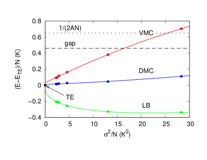
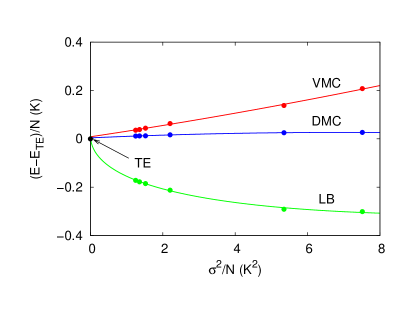
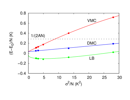
The lower bound, in turn, can be made stricter by extrapolation to zero variance of $E_{T}-\sqrt{\sigma^{2}}$ with a leading square-root term. These variance extrapolations are shown in Figs (3), (4) and (5) and listed in Table 1.

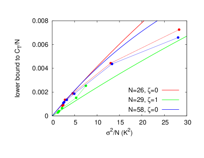
All of the above extrapolations are valid for $C_{T}\to 0$. Using a general estimate for the overlap of the trial wave function with the ground state xavier , $C_{T}\equiv 1-c_{0}^{2}\geq 1-\exp[-(E_{T}-E_{0})^{2}/2\sigma^{2}]\approx 1-\exp[-A^{2}\sigma^{2}]$, we can a-posteriori check the consistency of the energy versus variance extrapolation, see Fig. 6.

Finally, one would like to use variance extrapolation with the fixed-node energies to obtain even better results. However, within DMC, the variance $\langle\Psi_{DMC}|(H-E_{DMC})^{2}|\Psi_{DMC}\rangle$ is zero inside any nodal pocket DMCVariance and cannot be used anymore as a measure of the quality of the wave function. The most natural assumption is then to postulate that the variance $\sigma^{2}$ calculated in VMC is a good measure of the quality of the wave function in DMC as well. This allows us to use the same extrapolation for DMC energies as in the case of VMC, as shown in Figs. (3), (4) and (5), but without obtaining a lower bound. The DMC energy extrapolated to zero variance, listed in Table 1, happens to differ from the TE value by just the combined error bar, 10 mK for $\zeta=0$ and 4 mK for $\zeta=1$.

V Conclusions

In this paper we have introduced new, highly correlated wave functions for accurate descriptions of normal Fermi liquids based on generalized backflow coordinates which are iteratively improved. For liquid ³He at freezing density, the energy gain of these wave functions at the 4th iteration compared to the usual backflow trial wave function (0 iterations) is about $290$mK within VMC and $30$mK for FN-DMC. More important, we have shown that the true ground state energy can be obtained by variance extrapolation with intrinsic a-posteriori checks of the consistency and validity of the extrapolation. For small number of atoms, $N\sim 26$, we have shown that the obtained results are in agreement with unbiased calculations using transient estimates, but variance extrapolation can be used also to quantify the fixed-node error of larger systems. For systems with $N=58$ atoms, the fixed-node error of our best wave function is around $20$mK.

Thus, apart from significant VMC and FN-DMC energy gains, the iterative backflow renormalization procedure also leads to a general strategy to quantify the fixed-node error of the calculations. In combination with finite-size extrapolations based on the analytical informations contained in the trial wave function FSE ; FLP , the methods presented in the paper provide an important step towards the control of the accuracy of QMC calculations suffering from a Fermion sign problem.

Appendix A Computational details

Let us suppose that $q_{i}^{\alpha}$, are backflow coordinates $i=1,\dots N$ and $\alpha=1,\dots d$, where $d$ is the spatial dimension, and we have already computed the following partial derivatives

$$Q_{ij}^{\alpha\beta} \equiv \nabla_{i}^{\alpha}q_{j}^{\beta}$$ (12)

$$\widetilde{Q}_{j}^{\beta} \equiv \Delta q_{j}^{\beta}\equiv\sum_{i\alpha}\nabla_{i}^{\alpha}\nabla_{i}^{\alpha}q_{j}^{\beta}$$ (13)

We will further need

$$\overline{Q}_{lm}^{\beta\gamma}=\sum_{i\alpha}Q_{il}^{\alpha\beta}Q_{im}^{\alpha\gamma}$$ (14)

which is already needed for computation of the local energy of the Slater determinant using orbitals based on the above backflow coordinates Kwon93 , which we will shortly remind.

A.1 Backflow determinant

The gradient and the laplacian of a determinant, $D=\det\varphi_{ki}$, with backflow coordinates in the orbitals, $\varphi_{ki}\equiv\varphi_{k}({\bf q}_{i})$, can be calculated as follows

$$\nabla_{i}^{\alpha}\log D = \sum_{j\beta}F_{jj}^{\beta}Q_{ij}^{\alpha\beta}$$ (15)

$$\Delta\log D = \sum_{i\alpha}F_{ii}^{\alpha}\widetilde{Q}_{i}^{\alpha}+\sum_{i\alpha\beta}\left[\sum_{m}V_{im}\varphi_{mi}^{\alpha\beta}\right]\overline{Q}_{ii}^{\alpha\beta}$$ (16)

$$-\sum_{ij\alpha\beta}F_{ij}^{\alpha}F_{ji}^{\beta}\overline{Q}_{ji}^{\alpha\beta}$$

where

$$\varphi_{ki}^{\alpha}\equiv\frac{\partial\varphi_{ki}}{\partial q_{i}^{\alpha}},\quad\varphi_{ki}^{\alpha\beta}\equiv\frac{\partial^{2}\varphi_{ki}}{\partial q_{i}^{\alpha}\partial q_{i}^{\beta}},\quad F_{ij}^{\alpha}=\sum_{k}V_{ik}\varphi_{kj}^{\alpha}$$ (17)

and $V_{ik}$ is the inverse of the backflow matrix

$$V_{ik}=\frac{1}{D}\frac{\partial D}{\partial\varphi_{ki}},\quad\sum_{k}V_{ik}\varphi_{kj}=\delta_{ij}$$ (18)

The computational complexity is of order $N^{3}$ for the inversion of the orbital matrix, $V_{ik}$, as well as for the computation of the matrices $F_{ij}^{\alpha}$ and $\overline{Q}_{ij}^{\alpha\beta}$.

Note that this part of the calculations does not depend on the specific form of the backflow coordinates. The computation of the gradient and laplacian of the local energy based on Eq (15) and Eq (16) do only depend on the actual values of the orbital matrix, $\varphi_{ki}$, and its partial derivatives, Eqs. (17), and on the gradient and laplacian of the backflow coordinates, Eq (12) and Eq. (13). Therefore, Eq. (15) and Eq. (16) can be still used to calculate the local energy of determinants containing iterated backflow coordinates, as long as their derivatives are provided in the form of Eqs (12), (13), and (14).

A.2 Iterated Jastrow correlations

We can now build a Jastrow factor based on the distances between two quasi-particles,

$$U=\sum_{l<m}u(q_{lm})$$ (19)

where $u$ denotes the function and $u^{\prime}$ ($u^{\prime\prime}$) its first (second) derivative. The gradient of the Jastrow factor can then be calculated by the chain rule

$$\nabla_{i}^{\alpha}U=\sum_{l\beta}V_{l}^{\beta}Q_{il}^{\alpha\beta},\quad V_{l}^{\beta}=\sum_{m\neq l}\frac{u^{\prime}(q_{lm})}{q_{lm}}q_{lm}^{\beta}$$ (20)

and

$$\Delta U=\sum_{l\beta}V_{l}^{\beta}\widetilde{Q}_{l}^{\beta}+\sum_{l\neq m}\sum_{\beta\gamma}W_{lm}^{\beta\gamma}\left[\overline{Q}_{ll}^{\beta\gamma}-\overline{Q}_{lm}^{\beta\gamma}\right]$$ (21)

with

$$W_{lm}^{\beta\gamma}=\left(u^{\prime\prime}(q_{lm})-\frac{u^{\prime}(q_{lm})}{q_{lm}}\right)\frac{q_{lm}^{\beta}q_{lm}^{\gamma}}{q_{lm}^{2}}+\delta_{\beta\gamma}\frac{u^{\prime}(q_{lm})}{q_{lm}}$$ (22)

We see that the overall cost of the quasi-particle Jastrow factor and its derivatives needed for the local energy is of order of $N^{3}$, needed to build the matrix $\overline{Q}_{lm}^{\beta\gamma}$, Eq. (14). Since this matrix is already needed in the calculation of usual backflow wave function Kwon93 , the iterated Jastrow does not lead to a significant slow down compared to the usual backflow.

A.3 Iterated backflow coordinates

We now construct new backflow coordinates

$$y_{i}^{\alpha}=\sum_{j\neq i}q_{ij}^{\alpha}\eta(q_{ij})$$ (23)

where $\eta$ is the corresponding potential. In order to calculate the local energy for backflow orbitals in the Slater determinant based on $y_{i}^{\alpha}$, we need the following derivatives

$$Y_{ij}^{\alpha\beta}\equiv\nabla_{i}^{\alpha}y_{j}^{\beta},\quad\widetilde{Y}_{i}^{\alpha}\equiv\Delta y_{i}^{\alpha}$$ (24)

In order to calculate them, we will use the chain rule, based on the following partial derivatives

$$\frac{\partial y_{j}^{\beta}}{\partial q_{i}^{\alpha}} = \delta_{ij}\sum_{n}\dot{y}_{in}^{\alpha\beta}-\dot{y}_{ij}^{\alpha\beta}$$

$$\frac{\partial^{2}y_{k}^{\gamma}}{\partial q_{i}^{\alpha}\partial q_{j}^{\beta}} = \delta_{ijk}\sum_{n}\ddot{y}_{kn}^{\alpha\beta\gamma}-\delta_{jk}\ddot{y}_{ki}^{\alpha\beta\gamma}-\delta_{ij}\ddot{y}_{jk}^{\alpha\beta\gamma}-\delta_{ik}\ddot{y}_{kj}^{\alpha\beta\gamma}$$

where

$$\dot{y}_{ij}^{\alpha\beta} = \frac{\eta^{\prime}(q_{ij})}{q_{ij}}q_{ij}^{\alpha}q_{ij}^{\beta}+\eta(q_{ij})\delta_{\alpha\beta}$$

$$\ddot{y}_{ij}^{\alpha\beta\gamma} = \left[\eta^{\prime\prime}(q_{ij}-\frac{\eta^{\prime}(q_{ij})}{q_{ij}}\right]\frac{q_{ij}^{\alpha}q_{ij}^{\beta}q_{ij}^{\gamma}}{q_{ij}^{2}}$$

$$+\frac{\eta^{\prime}(q_{ij})}{q_{ij}}\left[q_{ij}^{\alpha}\delta_{\beta\gamma}+q_{ij}^{\beta}\delta_{\alpha\gamma}+q_{ij}^{\gamma}\delta_{\alpha\beta}\right]$$

and we have used that $\dot{y}_{ii}^{\alpha\beta}=\ddot{y}_{ii}^{\alpha\beta\gamma}=0$.

The final derivatives needed, Eqs. (24), can then be written as

$$Y_{ij}^{\alpha\beta} = \sum_{n\gamma}\dot{y}_{jn}^{\gamma\beta}\left[Q_{ij}^{\alpha\gamma}-Q_{in}^{\alpha\gamma}\right]$$

$$\widetilde{Y}_{i}^{\alpha} = \sum_{n\beta}\dot{y}_{in}^{\alpha\beta}\left[\widetilde{Q}_{i}^{\beta}-\widetilde{Q}_{n}^{\beta}\right]$$ (25)

$$+\sum_{n\alpha\beta}\ddot{y}_{in}^{\alpha\beta\gamma}\left[\overline{Q}_{ii}^{\beta\gamma}+\overline{Q}_{nn}^{\beta\gamma}-2\overline{Q}_{in}^{\beta\gamma}\right]$$

Again, these operations can be done in order of $N^{3}$ computations.

A.4 Iterated $n$-body correlations

Above we have explicitly shown how to calculate gradient and laplacian of a scalar two-body Jastrow potential and of quasi-particle coordinates constructed from backflow coordinates. The structure of our three-body correlation in Eq. (3) is actually a scalar product between two vectors with identical structure as the backflow coordinates. Gradient and laplacian of the three body term can therefore be calculated from those of the vectors using the chain rule. Generalizations to build iterated many-body Jastrow and backflow coordinates based on quasi-particle tensors BF3 are straightforward and do not increase the complexity of the calculation.

A.5 Higher order iterations

At the zeroth order of iteration, the backflow coordinates, ${\bf q}_{i}$, are symmetric functions of the bare coordinates. Higher order iterations of the backflow are built from symmetric expressions based on the previous backflow coordinates, such that the overall wave function remains antisymmetric. Above, we have explicitly shown how to calculate the gradient and the laplacian of the quasi-particle coordinates of the first backflow iteration, ${\bf q}_{i}^{(1)}\equiv{\bf q}_{i}+{\bf y}_{i}$ without increasing the overall complexity of the calculation. These are the only additional information needed to calculate the local energy of the first iterated backflow determinant, and from the structure it is clear that this procedure can be iterated to higher order without increasing the complexity of the calculations.

Figure 1: Optimized potentials of the trial function $\Psi_{T}^{(4)}$ for $N=26$, $\zeta=0$. The lines are broken where the pair distribution functions of the relevant (quasi)coordinates become negligibly small, $g(r)\lesssim 10^{-3}$ (see Fig. 2).

Figure 2: Pair correlation functions calculated in a VMC simulation with the BF⁽⁴⁾ trial function using the bare coordinates $\{{\bf r}_{i}\}$ (solid line), and the renormalized backflow coordinates $\{{\bf q}_{i}^{(0)}\}$, $\{{\bf q}_{i}^{(2)}\}$, and $\{{\bf q}_{i}^{(4)}\}$ (dotted, dash-dotted and dashed lines, respectively). The statistical noise reaches its maximum value $\sim 0.003$ at the highest peak.

Figure 3: The VMC and DMC energies per particle of $N=26$ unpolarized ³He atoms in two dimensions as a function of the variance $\sigma^{2}/N$. Each point corresponds to a different trial function (PW and BF^(α) with $\alpha=0$ to 4, from higher to lower variance). The TE energy has been subtracted. Their dependence is nearly linear, and their extrapolations to zero variance, the entries VMC_ext and DMC_ext of Table 1, are very close to the exact result. We further show the energy lower bound $(E_{T}-\sqrt{\sigma^{2}})/N$, whose extrapolation to zero variance, the entry LB_ext of Table 1, is also very close to the exact result. The dashed line is a rough estimate of the first excited state (the difference between the two slowest exponential decay constants in the fermionic signal of the TE procedureCarleo ). It shows that the condition for the validity of the energy lower bound (see text) are met by the iterated backflow trial functions. The dotted line is the alternate estimate $1/(2AN)$ of Eq. (11) for the validity of the lower bound.

Figure 4: Same as Fig. 3, for $N=29$ spin-polarized ³He atoms. Both the estimate of the first excited state, $\sim 0.6$ K, and the value of $1/(2AN)$, 0.772 K, are off scale.

Figure 5: Same as Fig. 3, for $N=58$ unpolarized ³He atoms. In the lack of TE results, we take a reference energy $E_{0}/N$ halfway between VMC_ext and LB_ext. Also, we do not have an estimate of the first excited state. Comparison of the dotted line with that of Fig. 3 shows that the range of $E_{T}-E_{0}$ where the lower bound is expected to be valid shrinks as $1/N$.

Figure 6: Points connected by thin lines : the lower bound $\{1-\exp[-(E_{T}-E_{0})^{2}/2\sigma^{2}]\}/N$ to the missing overlap per particle between trial function and ground state, $C_{T}/N$ (with $E_{0}$ replaced by the zero-variance extrapolation of $E_{T}$). The points refer to trial functions from PW to BF⁽⁴⁾, in order of decreasing variance. Thick lines: the approximation $\{1-\exp[-A^{2}\sigma^{2}]\}/N$ obtained using only the linear term of the fit of energy vs. variance.

References

- (1) P.J. Reynolds, D.M. Ceperley, B.J. Alder, and W.A. Lester, J. Chem. Phys. 77, 5593 (1982).
- (2) D.M. Ceperley and B.J. Alder, J. Chem. Phys. 81, 5833 (1984).
- (3) G. Carleo, S. Moroni, F. Becca, and S. Baroni, Phys. Rev. B 83, 060411(R) (2011).
- (4) M. Nava, A. Motta, D. E. Galli, E. Vitali, and S. Moroni Phys. Rev. B 85, 184401 (2012).
- (5) J. J. Shepherd, G. Booth, A. Grüneis, and A. Alavi, Phys. Rev. B 85, 081103(R) (2012).
- (6) F. Pederiva, S. A. Vitiello, K. Gernoth, S. Fantoni, and L. Reatto, Phys. Rev. B 53, 15129 (1996); F. Calcavecchia, F. Pederiva, M. H. Kalos, and T. D. Kühne, arXiv:1404.6944 (2014).
- (7) V. R. Pandharipande and N. Itoh, Phys. Rev. A 8, 2564 (1973).
- (8) K. E. Schmidt and V. R. Pandharipande, Phys. Rev. B 19, 2504 (1979).
- (9) E. Manousakis, S. Fantoni, V. R. Pandharipande, and Q. N. Usmani, Phys. Rev. B 28, 3770 (1983).
- (10) S. A. Vitiello, K. E. Schmidt, and S. Fantoni, Phys. Rev. B 55, 5647 (1997).
- (11) Y. Kwon, D. M. Ceperley and R. M. Martin, Phys. Rev. B 48, 12037 (1993).
- (12) Y. Kwon, D. M. Ceperley and R. M. Martin, Phys. Rev. B 58 6800 (1998).
- (13) M. Holzmann, D. M. Ceperley, C. Pierleoni and K. Esler, Phys. Rev. E68, 046707 (2003).
- (14) K. E. Schmidt, M. A. Lee, M. H. Kalos, and G.V. Chester, Phys. Rev. Lett. 47, 807 (1981).
- (15) R. M. Panoff and J. Carlson, Phys. Rev. Lett. 62, 1130 (1989).
- (16) J. Casulleras and J. Boronat, Phys. Rev. Lett. 84, 3121 (2000).
- (17) S. Moroni, S. Fantoni, and G. Senatore, Phys. Rev. B 52, 13547 (1995).
- (18) F.H. Zong, D.M. Ceperley, S. Moroni, and S. Fantoni, Mol. Phys. 101, 1705 (2003).
- (19) M. Holzmann, B. Bernu, and D.M. Ceperley, Phys. Rev. B 74, 104510 (2006).
- (20) W.L. McMillan, Phys. Rev. 138, A442 (1965).
- (21) E. Feenberg, Theory of Quantum Fluids, Academic, New York (1969).
- (22) E. Krotscheck in Introduction to modern methods of quantum many-body theory and their applications, A. Fabrocini, S Fantoni, and E. Krotscheck (ed.), World Scientific Singapore (2002).
- (23) R. A. Aziz, V. P. S. Nain, J. S. Carley, W. L. Taylor and G. T. McConville, J. Chem. Phys 70, 4330 (1979). The potential is made to vanish at half the side of the simulation box by a rigid shift.
- (24) D. M. Ceperley and M. H. Kalos in Monte Carlo Methods in Statistical Physics, K. Binder (ed.), Springer-Verlag, 1979.
- (25) G. Temple, Proc. Roy. Soc. Ser. A 119, 276 (1928).
- (26) C. Mora and X. Waintal, Phys. Rev. Lett. 99, 030403 (2007).
- (27) Unless the nodes are exact, the FN-DMC wave function will have a discontinuous derivative at the nodal surface. Nevertheless, one can show that the energy expectation value of a FN-DMC wave function still provides an upper bound to the true ground state wave function having continuous derivatives everywhere.
- (28) S. Chiesa, D.M. Ceperley, R.M. Martin, and M. Holzmann, Phys. Rev. Lett. 97, 076404 (2006).
- (29) M. Holzmann, B. Bernu, V. Olevano, R.M. Martin, and D.M. Ceperley, Phys. Rev. B 79, 041308(R) (2009); M. Holzmann, B. Bernu, C. Pierleoni, J. McMinis, D. M. Ceperley, V. Olevano, and L. Delle Site, Phys. Rev. Lett. 107, 110402 (2011).