Static pair free energy and screening masses from correlators of Polyakov loops: continuum extrapolated lattice results at the QCD physical point
Abstract
We study the correlators of Polyakov loops, and the corresponding gauge invariant free energy of a static quark-antiquark pair in 2+1 flavor QCD at finite temperature. Our simulations were carried out on lattices using Symanzik improved gauge action and a stout improved staggered action with physical quark masses. The free energies calculated from the Polyakov loop correlators are extrapolated to the continuum limit. For the free energies we use a two step renormalization procedure that only uses data at finite temperature. We also measure correlators with definite Euclidean time reversal and charge conjugation symmetry to extract two different screening masses, one in the magnetic, and one in the electric sector, to distinguish two different correlation lengths in the full Polyakov loop correlator.
1 Introduction
At high temperatures strongly interacting matter undergoes a
transition where colorless hadrons turn into a phase dominated by
colored quarks and gluons, the quark gluon plasma (QGP). Recently, lattice simulations
have shown that this transition is a crossover Aoki et al. (2006a) and its
characteristic temperature has also been
determined Cheng et al. (2006); Aoki et al. (2006b, 2009); Borsanyi et al. (2010); Bazavov et al. (2012).
Deconfinement properties of the transition can be studied by
infinitely heavy, static test charges. At zero temperature a heavy quark and antiquark pair forms a
bound state (quarkonium state), but above the deconfinement temperature,
color screening and collisions with the medium would reduce the binding between the quark
and the antiquark, eventually causing a dissociation.
As proposed by Ref. Matsui and Satz (1986),
the behavior of quarkonia can signal deconfinement and QGP production
in heavy ion experiments. Moreover, the different melting temperatures of the different states
can be used as a thermometer, analogously to the spectral analysis of stellar media in astrophysics,
where the absence and presence of the different spectral lines is used to determine the temperature.
In medium quarkonium properties are characterized by the corresponding spectral functions,
studied in several works. However, extracting spectral functions from Euclidean meson
correlators (i.e. the analytic continuation of the correlator to real time) is a difficult,
ill-posed problem. Nevertheless, lattice studies of charmonium spectral functions
using the Maximum Entropy Method have been carried out on numerous
occasions Jakovac et al. (2007); Umeda et al. (2005); Asakawa and Hatsuda (2004); Iida et al. (2006); Ohno et al. (2011); Ding et al. (2012); Aarts et al. (2007); Kelly et al. (2013); Borsanyi et al. (2014a); Aarts et al. (2013a, b); Kim et al. (2013).
A recent, detailed study of charmonium spectral functions in
quenched QCD can be found in Ding et al. (2012). Results regarding spectral functions
with 2 flavours of dynamical quarks can be found in Refs. Aarts et al. (2007); Kelly et al. (2013).
A recent study of charmonium spectral functions in 2+1 flavour QCD is Borsanyi et al. (2014a, b). Bottomonium
spectral functions have also been studied with the help of
NRQCD Aarts et al. (2013a, b); Kim et al. (2013).
Since the direct determination of the spectral function is difficult, one can study
in-medium properties of quarkonium using approximate potential models.
There are numerous proposals in the literature for lattice observables which can provide
input to these models. The so-called singlet and octet potentials have been
proposed Nadkarni (1986a); Kaczmarek et al. (2002, 2004); Kaczmarek and Zantow (2005); Mocsy and Petreczky (2008),
and studied on the lattice, but these are not gauge invariant, therefore
extracting physical information from them is not straightforward. There was also a suggestion about
using the analytic continuation of the Wilson-loop Laine et al. (2007); Rothkopf et al. (2012), that, however,
has similar problems as the direct reconstruction of the spectral functions. Here, we calculate the gauge
invariant static quark-antiquark pair free energy, a non-perturbatively well defined quantity,
that carries information on the deconfinement properties of the QGP.
In the present paper we determine the free energy of a static quark-antiquark pair as a function of their distance at various temperatures. We accomplish it by measuring the Polyakov loop correlator McLerran and Svetitsky (1981), which gives the gauge invariant free energy 111More precisely, the excess free energy that we get when inserting two static test charges in the medium. as:
| (1) |
In the above formula, x runs over all the lattice spatial sites, and the Polyakov loop, , is defined as the product of temporal link variables 222In the literature, a factor of is often included in the definition. Including this factor leads to a term in the static quark free energy that is linear in temperature.:
| (2) |
or in the continuum formulation, as a path ordered exponential of the integral of the gauge fields:
| (3) |
The leading order term to the correlator of Polyakov loops is
a two gluon exchange diagram. It was first calculated at leading order
in the dimensionally reduced effective theory (EQCD3) Nadkarni (1986b).
Due to the two gluon exchange, the dependence in leading order
is , where is the Debye screening mass. This suggests
that in the limit, where perturbation
theory is applicable, the correlator should behave as . However, this is not the asymptotic
behavior, which we need to fit the correlation length on the lattice. The reason is simple:
even in the weak coupling limit, at distances larger than the physics of magnetic screening
becomes dominant. From the then applicable 3D effective pure Yang-Mills theory, Ref. Braaten and Nieto (1995) argued
that at high temperature, the large distance behavior is , where is the magnetic
screening mass. This was confirmed by 2 flavour lattice simulations (using a somewhat heavy pion) in Maezawa et al. (2010).
A related problem is that for the gluon self-energy, perturbation theory breaks down at the order because of infrared divergences. This term contains contributions from magnetic gluons. Therefore, the perturbative definition of the screening mass, as a pole in the gluon propagator, is of limited use, since pertubation theory breaks down (Arnold and Yaffe (1995)). It is better to define the screening masses as inverse correlation lengths in appropriate Euclidean correlators. In order to investigate the effect of electric and magnetic gluons separately, one can use the symmetry of Euclidean time reflection Arnold and Yaffe (1995), that we will call . The crucial property of magnetic versus electric gluon fields and is that under this symmetry, one is intrinsically odd, while the other is even:
| (4) |
Under this symmetry the Polyakov loop transforms as . One can easily define correlators that are even or odd under
this symmetry, and thus receive contributions only from the magnetic or electric sector,
respectively Arnold and Yaffe (1995); Maezawa et al. (2010):
| (5) | |||
| (6) |
We can further decompose the Polyakov loop into even and odd states, using and as:
| (7) | |||
| (8) |
Next, we note that , so the decomposition of the Polyakov loop correlator to definite and symmetric operators contains two parts333Note that the Polyakov loop correlator does not overlap with the and sectors. To access these sectors, other operators are needed.. We define the magnetic correlation function as:
| (9) |
and the electric correlator as444Here our definition differs from that used in Maezawa et al. (2010) in a sign.:
| (10) |
Then, from the exponential decay of these correlators, we can define the magnetic and electric screening masses. Note that with our definition and , and:
| (11) |
from which it trivially follows that if the magnetic mass screening mass is lower than the electric mass, we will
have asymptotic to as , or equivalently, the highest
correlation length in equal to that of .
As for the asymptotic form of these correlators, similar arguments apply as with the full Polyakov loop correlator. In the high temperature limit the asymptotic behavior will be dominated by a glueball mass in the 3D effective Yang-Mills theory Arnold and Yaffe (1995); Braaten and Nieto (1995), but because of the symmetry properties, the quantum numbers carried by the glueballs will be different. We will therefore fit the ansatz:
| (12) | |||
| (13) |
to extract screening masses, noting that the ansatz in principle is only motivated at high temperatures, where the effective field theory applies. Nevertheless we find that even close to the ansatz describes the large tails of our lattice data well.
2 Simulation details
The simulations were performed by using the tree level Symanzik improved gauge,
and stout-improved staggered fermion action, that was used in Aoki et al. (2006c).
We worked with physical quark masses, and fixed them by reproducing the
physical ratios and Aoki et al. (2006c).
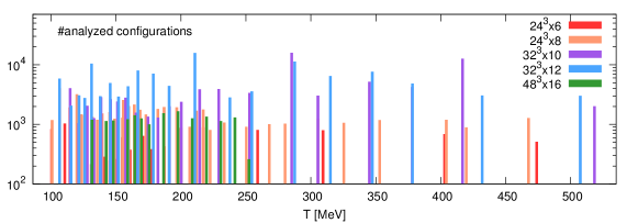
Compared to our previous investigations of Polyakov loop correlators, reported in the conference proceedings Fodor et al. (2007), here we used finer lattices, namely we carried out simulations on and lattices as well as on lattices. Our results were obtained in the temperature range 150 MeV T 450 MeV. We use the same configurations as in Ref. Borsanyi et al. (2010) and Borsanyi et al. (2014c). Figure 1 summarizes our statistics.
3 The gauge invariant free energy
3.1 Renormalization procedure and continuum extrapolation
After measuring the Polyakov loop correlator at temperature, we
computed the unrenormalized free energy according to .
The function was taken from the
line of constant physics, along which we kept the ratios of the physical
values of , and fixed at zero temperature. Detailed
description of the determination of the line of constant physics can be
found in Ref. Borsanyi et al. (2014c).
Approaching the continuum limit, the value of the unrenormalized free energy diverges. In order to eliminate the divergent part of the free energy renormalization is needed. There are various proposals in the literature for this renormalization procedure. Earlier works Kaczmarek et al. (2002, 2004); Kaczmarek and Zantow (2005) matched the short distance behavior to the static potential, but this is ambiguous. A more precise definition is to require that the potential vanishes at some distance Aoki et al. (2006b); Fodor et al. (2007). This would require a precise determination of the potential at . Here, though, we use a renormalization procedure based entirely on our data, similarly to Ref. Borsanyi et al. (2012). The data contains a temperature independent divergent part from the ground state energy. The difference between the value of free energies at different temperatures is free of divergences. Accordingly, we define the renormalized free energy as:
| (14) |
with a fixed . This renormalization prescription corresponds to the choice that the free energy at large distances goes to zero at , and is implemented in two steps. In the first step we have:
| (15) |
where the one quark free energy satisfies:
| (16) |
Note, that this first step of the renormalization procedure is completely straightfoward to implement, at each simulation point in and we just subtract the asymptotic value of the correlator. This gives us a UV finite quantity , however we don’t call this the renormalized free energy, since compared to equation (14) it contains less information. Namely at all temperatures . The correlation length is the same as with definition (14), but the information of the asymptotic value (that is the single heavy quark free energy) is lost. That information however is retained in the second step:
| (17) |
where the renormalized one heavy quark free energy is:
| (18) |
Doing the renormalization in two steps like this has a technical reason that will be explained shortly.
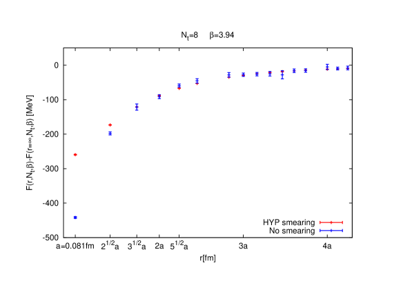
Let us first mention that this Polyakov loop correlator behaves similarly to the baryon correlators in imaginary time do: at large values of we can get negative values of at some configurations555Of course, the ensemble average should in principle be positive definite.. For this reason, it is highly desirable to use gauge field smearing which makes for a much better behavior at large , at the expense of unphysical behavior at small . For this reason, we measured the correlators both without and with HYP smearing. We expect that outside the smearing range (i.e. ) the two correlators coincide. This is supported by Figure 2. Therefore we use the smeared correlators for and the unsmeared ones for .
3.1.1 Single heavy quark free energy
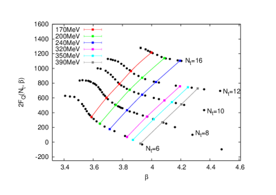
First, we discuss the implementation of the renormalization of the single heavy quark free energy, equation (18). Notice that if we implemented the renormalization condition (14) directly, then we would just need to subtract from the unrenormalized free energy, so at first sight it looks like we are doing some unnecessary rounds by doing this in two steps. What we gain by this is that we can extend the temperature range, at which we can do the continuum limit. To understand this statement let us look at Figure 3 (left). The dotted black symbols are bare values of at given values of and . The colored symbols are interpolations of these curves, in to the value of corresponding to the temperature at each . If we take for example , corresponding to the green line in the figure, this gives us 5 points from the curve . According to equation (18) this is what we have to subtract from the bare free energy at this value of to get the renormalized single quark free energy. The disadvantage of the green curve, is that the range it covers is rather limited. So, if we want to be able to make a continuum limit from say the lattices, the temperature range we can cover is rather limited as well. The lowest temperature we will be able to do a continuum limit at will be , and the highest temperature will be .To do a continuum limit at higher temperatures, we need the curve at higher values of , and at first, it looks as like that would need runs at higher values of . This is not feasible, but there is a simple tricj to extend the temperature range. Clearly, if we call the continuum limit of the single quark free energy
| (19) |
than, for any value of :
| (20) |
is just a number666This statement is only true in the continuum. At finite lattice spacing there is also a lattice spacing
dependent artifact in this difference.. We can use this fact to extend the temperature range of the continuum limit by using different
values of , that is different renormalization prescriptions, and shift them together by the value of the RHS of equ. (20).
This is the procedure that we will follow.
To implement equation (18), we first calculate or equivalently
from equation (16). Then at each we interpolate to the value corresponding to the temperature , giving us some
points of the function . Finally, we interpolate these points in , obtaining
the final curve we can use for the renormalization. This procedure is illustrated on Figure 3 (left).
When doing this interpolation we take into
account the error on the data points of
via the jacknife method. The statistical errors of the single quark free energy are very
small, meaning that the interpolation method gives a comparable error to the final interpolated value. We estimate the systematic error of
the interpolations by constructing different interpolations. For interpolations of the curves we use linear
and cubic spline interpolations (for each value of ), and for the interpolation of we use different polynomial
interpolations(order 1,2), cubic spline and barycentric rational function interpolation. In total this means different
interpolations, than for interpolating the bare we use spline and linear interpolations, so for
the final renormalized values we have in total different interpolations. All interpolations are
taken to have the same weight. We use the median of this as the estimate, and the
symmetric median centered 68% as the 1σ systematic error estimate Durr et al. (2008). The statistical
and systematic errors turn out to be of the same order, and are than added in quadrature.
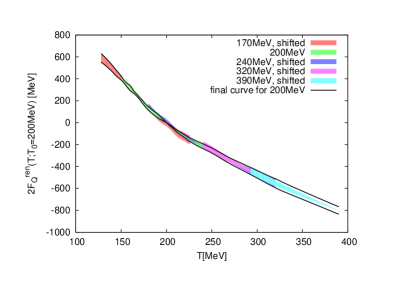
After doing this procedure, the range in which we can interpolate the curve is limited, therefore, the temperature
range where we can do the continuum extrapolation is limited. To extend the temperature range where we can calculate
the single heavy quark free energy, we use the fact that the single heavy quark free energies
at different temperatures differ only by an additive constant in the continuum. Therefore
we use different values of to do the continuum extrapolation, and shift all those curves to the position of the
curve. We used 5 different values of , namely, MeV, MeV, MeV, MeV, and MeV.
The results of this analysis can be found in Figure 3 (right).
For the continuum limits, we use the lattices, that are available at all temperatures. We use the lattice to estimate the systematic error of the continuum extrapolation, where it is available. If:
then the systematic error of the continuum extrapolation is taken to be . Where
the lattices are not available,
we approximate the relative systematic error by the average of the systematic errors at the parameter values where we had the
lattices available. This corresponds to an error level of approximately .
The systematic and statistical errors of the
continuum extrapolations are then added in quadrature. The linear
fits of the continuum limit extrapolations all have good values of .
Finally, we mention that the determination of the continuum limit of the Polyakov loop, or equivalently, that single static quark free energy is already available in the literature. For two recent determinations of the Polyakov loop see Refs. Borsanyi et al. (2010); Bazavov and Petreczky (2013). The difference is that here we take the continuum limit at significantly higher temperatures.
3.1.2 Heavy pair free energy
Next, we turn to the determination of defined in equation 15. This quantity is UV finite, and goes
to 0 as . Similarly to the single quark free energy, the determination of at a given value of
and requires two interpolations. At first we are given at several values of , at each we have a different
value of the lattice spacing. If we want to know the value of at at some value of ,
first we do an interpolation in the direction to the value at each given , then we do an interpolation in the T direction, where the node
points for the interpolations are the interpolants in the previous step. The statistical error than can be estimated by constructing these
interpolations to every jacknife sample. For systematic error estimation we try different interpolations in the and directions.
In the r direction we have: polynomials of order 1,2,3,…,7 and a cubic spline, in the direction we have polynomials of order 1,2,3 and
cubic spline. This is in total different interpolations. Just as before, we use the median of these values as
the estimate, and the symmetric median centered as the systematic error estimate. Like in the case of the
single heavy quark free energies, the statistical and systematic errors turn out to be of the same order, and are then added in quadrature.
Next, we do the continuum extrapolation. Here we also take a similar approach as in the previous subsection.
For the continuum extrapolations, we use the lattices, that are available at all temperatures. We use the
lattice to estimate the systematic error of the continuum extrapolation, exactly like before. Also, where the
lattices are not available, we estimate the systematic error, as in the previous section, by the average of the systematic
error at the points where we do have lattices (approximately ). The linear fits of the continuum limit extrapolations all
have good values of .
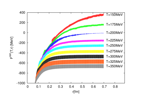
Next, we add the values of , determined in the previous subsection, and visible in Figure 3 to the free energy values to obtain the final results in Figure 4 (errors are added in quadrature). Note, that the lattices were only used in the whole analysis to extend the range of the renormalization condition for the single quark free energy.
4 Magnetic and electric screening masses
We continue with the discussion of the electric and magnetic screening masses obtained from the correlators
(9) and (10). For this analysis we only use lattices above the (pseudo)critical
temperature, since that is the physically interesting range for screening. Next, we mention that for this analysis,
we only use the data with HYP smearing, since we are especially interested in the large r behavior. Before
going on to the actual fitting procedure of the screening masses let us first illustrate some simple relations,
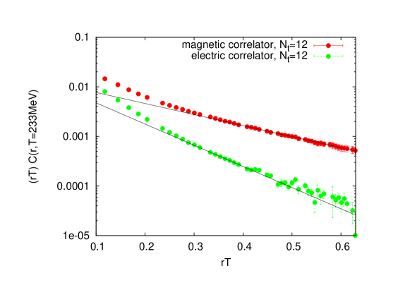
with the raw lattice data of the electric and magnetic correlators. First as ,
or equivalently, that the electric screening mass is larger than the magnetic one. This can be seen on Figure 5.
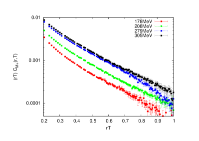
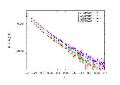
The next observation is that the screening masses in both channels are approximately proportional to the temperature.
This can be seen on Figure 6. Both of these facts are expected to hold at high temperatures, but
these lattice results suggest that they hold at lower
temperatures as well.
Next, we turn to the actual determination of the screening masses.
So far there has been one determination of electric and magnetic screening masses on the lattice
using the non-perturbative definition given by ref. Arnold and Yaffe (1995). That study used
2 flavours of Wilson fermions with a somewhat heavy pion, and did not attempt a continuum extrapolation Maezawa et al. (2010).
| Correlator type | |||
| Magnetic | 0.007 | ||
| Magnetic | 0.016 | ||
| Magnetic | 0.30 | ||
| Magnetic | 0.38 | ||
| Magnetic | 0.96 | ||
| Electric | |||
| Electric | 0.018 | ||
| Electric | 0.31 | ||
| Electric | 0.94 |
Since the masses are expected to be proportional to the temperature, the natural distance unit in this problem is , so we give limits on the range of the fits in these units. For the correct determination of the screening masses, special care is needed in the choice of the fit interval. To find the proper minimum value of the fits, we use hypothesis testing, similar to that in Ref. Borsanyi et al. (2014d). If the fits are good, than the value of , defined as:
| (21) |
should have a distribution, with the appropriate degrees of freedom. Here is the covariance matrix. In this case the quantity
| (22) |
should have a uniform distribution on . If we fix the range of all the fits in units, each fit
(at some value of and ) gives one pick from a supposed uniform distribution in Q. This is
equivalent to having multiple picks from the same uniform distribution. We will test this hypothesis with
a Kolmogorov-Smirnov test for the uniform distribution. Here one determines the maximum value of the absolute
difference between the expected and measured cumulative probability distributions. This is then used to define a significance
level or probability that the measured distribution can indeed be one originating from the expected uniform distribution.
These probabilities are listed in Table 1. We will only use value of where the Kolmogorov
probability is at least . This test tells us, that for systematic error estimation, we will have, for the magnetic
correlator going from 0.465 to 0.61,
and for the electric correlator we have going from 0.35 to 0.43
777 was fixed on both cases. Increasing results in
a less precise covariance matrix and correspondingly, somewhat worse values, but consistent screening masses.
For example, if for the magnetic correlator we choose instead of , the final value of the
Kolmogorov-Smirnov probability in Table 1 will not be , but instead. Nevertheless the growing trend
in the probabilities will be the same. Also, we will get the same results within uncertainties..
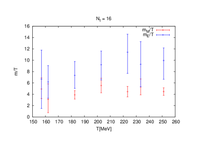
At this point we mention that for the continuum limit we will not use the lattices, because the
mass fits there have huge error bars. Nevertheless, when the continuum limit is done, we will see that
the values of the masses at the lattices are consistent with the continuum estimates. Also, if we use them,
we get the same results, because they do not give a contribution to the continuum limit, due to the big errors.
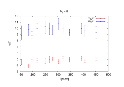
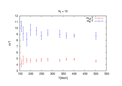
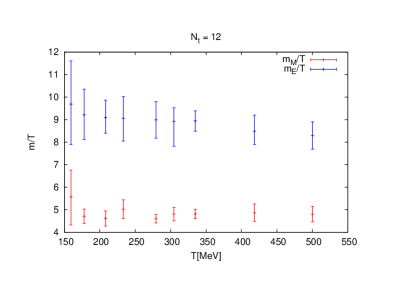
Now that we have estimated the proper range of the fits, we go on to the fitting of the masses.
The results of the fits at different
values of can be seen in Figure 7.
The systematic errors come from changing the lower limit of the fit, in the case of the magnetic
correlator, from to , and in the case of the electric correlator, from to
. The results coming from different values of are weighted using
the Akaike Information Criterion(AIC) Akaike (1974). The median of the weighted histogram gives the central value,
and the central the systematic error estimate. Note that using the Q values as weights or uniform weights
gives a very similar result.
The statistical error comes from a jacknife analysis with 20 jacknife samples.
The two errors turn out to be of similar magnitude (with the statistical error being somewhat bigger) and are then added
in quadrature.
Next, we fit linear functions to all screening masses at all values of ,
and use these to do a continuum extrapolation from the lattices.
Taking into account the errors of the linear fits, all values of the continuum limits are very good. The continuum limit, in addition to the statistical
error, also has a systematic error estimated, from doing a 2 point linear extrapolation from the lattices, and taking the
difference of the extrapolated value from fitted value to the lattices888In the previous section, we used
the lattices for systematic error estimation, here however, we do not use them since they do not improve the
statistical accuracy of the continuum limits.. The statistical and systematic errors are added in quadrature.
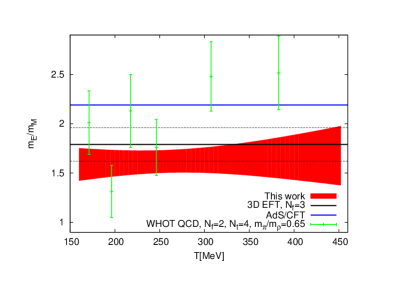
We finish this section by comparing our results to those from earlier approximations in the literature. For comparison let us use our results at . Here we have:
-
•
This work: 2+1 flavour lattice QCD at the physical point after continuum extrapolation:
-
•
Ref. Maezawa et al. (2010): 2 flavour lattice QCD with Wilson quarks, a somewhat heavy pion , no continuum extrapolation
-
•
From Table 1 of Ref. Bak et al. (2007): SYM, large limit, AdS/CFT
-
•
From Figure 3 of Ref. Hart et al. (2000): dimensionally reduced 3D effective theory, massless quarks
-
•
From Figure 3 of Ref. Hart et al. (2000): dimensionally reduced 3D effective theory, massless quarks
We note, that our results are closest to the results from dimensionally reduced effective field theory.
5 Conclusions
In this paper we have determined the renormalized static quark-antiquark free energies in the continuum limit. We introduced a two step renormalization procedure using only the finite temperature results. The low radius part of the free energies tended to the same curve, corresponding to the expectation that at small distances, the physics is temperature independent. We also calculated the magnetic and electric screening masses, from the real and imaginary parts of the Polyakov loop respectively. As expected, both of these masses approximately scale with the temperature as , with , therefore, magnetic contributions dominating at high distances. The values we got for the screening masses are close to the values from dimensionally reduced effective field theory.
Acknowledgment
Computations were carried out on GPU clusters Egri et al. (2007) at the
Universities of Wuppertal and Budapest as well as on supercomputers in
Forschungszentrum Juelich.
This work was supported by the DFG Grant SFB/TRR 55, ERC no. 208740. and
the Lendulet program of HAS (LP2012-44/2012).
References
- Aoki et al. (2006a) Y. Aoki, G. Endrodi, Z. Fodor, S.D. Katz, and K.K. Szabo. The Order of the quantum chromodynamics transition predicted by the standard model of particle physics. Nature, 443:675–678, 2006a. doi: 10.1038/nature05120.
- Cheng et al. (2006) M. Cheng, N.H. Christ, S. Datta, J. van der Heide, C. Jung, et al. The Transition temperature in QCD. Phys.Rev., D74:054507, 2006. doi: 10.1103/PhysRevD.74.054507.
- Aoki et al. (2006b) Y. Aoki, Z. Fodor, S.D. Katz, and K.K. Szabo. The QCD transition temperature: Results with physical masses in the continuum limit. Phys.Lett., B643:46–54, 2006b. doi: 10.1016/j.physletb.2006.10.021.
- Aoki et al. (2009) Y. Aoki, Szabolcs Borsanyi, Stephan Durr, Zoltan Fodor, Sandor D. Katz, et al. The QCD transition temperature: results with physical masses in the continuum limit II. JHEP, 0906:088, 2009. doi: 10.1088/1126-6708/2009/06/088.
- Borsanyi et al. (2010) Szabolcs Borsanyi et al. Is there still any mystery in lattice QCD? Results with physical masses in the continuum limit III. JHEP, 1009:073, 2010. doi: 10.1007/JHEP09(2010)073.
- Bazavov et al. (2012) A. Bazavov, T. Bhattacharya, M. Cheng, C. DeTar, H.T. Ding, et al. The chiral and deconfinement aspects of the QCD transition. Phys.Rev., D85:054503, 2012. doi: 10.1103/PhysRevD.85.054503.
- Matsui and Satz (1986) T. Matsui and H. Satz. J/ Suppression by Quark-Gluon Plasma Formation. Phys.Lett., B178:416, 1986. doi: 10.1016/0370-2693(86)91404-8.
- Jakovac et al. (2007) A. Jakovac, P. Petreczky, K. Petrov, and A. Velytsky. Quarkonium correlators and spectral functions at zero and finite temperature. Phys.Rev., D75:014506, 2007. doi: 10.1103/PhysRevD.75.014506.
- Umeda et al. (2005) Takashi Umeda, Kouji Nomura, and Hideo Matsufuru. Charmonium at finite temperature in quenched lattice QCD. Eur.Phys.J., C39S1:9–26, 2005. doi: 10.1140/epjcd/s2004-01-002-1.
- Asakawa and Hatsuda (2004) M. Asakawa and T. Hatsuda. J / psi and eta(c) in the deconfined plasma from lattice QCD. Phys.Rev.Lett., 92:012001, 2004. doi: 10.1103/PhysRevLett.92.012001.
- Iida et al. (2006) H. Iida, T. Doi, N. Ishii, H. Suganuma, and K. Tsumura. Charmonium properties in deconfinement phase in anisotropic lattice QCD. Phys.Rev., D74:074502, 2006. doi: 10.1103/PhysRevD.74.074502.
- Ohno et al. (2011) H. Ohno et al. Charmonium spectral functions with the variational method in zero and finite temperature lattice QCD. Phys.Rev., D84:094504, 2011. doi: 10.1103/PhysRevD.84.094504.
- Ding et al. (2012) H.T. Ding, A. Francis, O. Kaczmarek, F. Karsch, H. Satz, et al. Charmonium properties in hot quenched lattice QCD. Phys.Rev., D86:014509, 2012. doi: 10.1103/PhysRevD.86.014509.
- Aarts et al. (2007) Gert Aarts, Chris Allton, Mehmet Bugrahan Oktay, Mike Peardon, and Jon-Ivar Skullerud. Charmonium at high temperature in two-flavor QCD. Phys.Rev., D76:094513, 2007. doi: 10.1103/PhysRevD.76.094513.
- Kelly et al. (2013) Aoife Kelly, Jon-Ivar Skullerud, Chris Allton, Dhagash Mehta, and Mehmet B. Oktay. Spectral functions of charmonium from 2 flavour anisotropic lattice data. PoS, LATTICE2013:170, 2013.
- Borsanyi et al. (2014a) Szabolcs Borsanyi, Stephan Durr, Zoltan Fodor, Christian Hoelbling, Sandor D. Katz, et al. Charmonium spectral functions from 2+1 flavour lattice QCD. JHEP, 1404:132, 2014a. doi: 10.1007/JHEP04(2014)132.
- Aarts et al. (2013a) Gert Aarts, Chris Allton, Seyong Kim, Maria Paola Lombardo, Mehmet B. Oktay, et al. S wave bottomonium states moving in a quark-gluon plasma from lattice NRQCD. JHEP, 1303:084, 2013a. doi: 10.1007/JHEP03(2013)084.
- Aarts et al. (2013b) G. Aarts, C. Allton, S. Kim, M.P. Lombardo, S.M. Ryan, et al. Melting of P wave bottomonium states in the quark-gluon plasma from lattice NRQCD. JHEP, 1312:064, 2013b. doi: 10.1007/JHEP12(2013)064.
- Kim et al. (2013) Seyong Kim, Peter Petreczky, and Alexander Rothkopf. Lattice NRQCD study of in-medium bottomonium states using HotQCD configurations. 2013.
- Borsanyi et al. (2014b) Szabolcs Borsanyi, Stephan Dürr, Zoltán Fodor, Christian Hoelbling, Sándor D. Katz, et al. Spectral functions of charmonium with 2+1 flavours of dynamical quarks. 2014b.
- Nadkarni (1986a) Sudhir Nadkarni. Nonabelian Debye Screening. 2. The Singlet Potential. Phys.Rev., D34:3904, 1986a. doi: 10.1103/PhysRevD.34.3904.
- Kaczmarek et al. (2002) O. Kaczmarek, F. Karsch, P. Petreczky, and F. Zantow. Heavy quark anti-quark free energy and the renormalized Polyakov loop. Phys.Lett., B543:41–47, 2002. doi: 10.1016/S0370-2693(02)02415-2.
- Kaczmarek et al. (2004) O. Kaczmarek, F. Karsch, F. Zantow, and P. Petreczky. Static quark anti-quark free energy and the running coupling at finite temperature. Phys.Rev., D70:074505, 2004. doi: 10.1103/PhysRevD.70.074505,10.1103/PhysRevD.72.059903.
- Kaczmarek and Zantow (2005) Olaf Kaczmarek and Felix Zantow. Static quark anti-quark interactions in zero and finite temperature QCD. I. Heavy quark free energies, running coupling and quarkonium binding. Phys.Rev., D71:114510, 2005. doi: 10.1103/PhysRevD.71.114510.
- Mocsy and Petreczky (2008) Agnes Mocsy and Peter Petreczky. Can quarkonia survive deconfinement? Phys.Rev., D77:014501, 2008. doi: 10.1103/PhysRevD.77.014501.
- Laine et al. (2007) M. Laine, O. Philipsen, P. Romatschke, and M. Tassler. Real-time static potential in hot QCD. JHEP, 0703:054, 2007. doi: 10.1088/1126-6708/2007/03/054.
- Rothkopf et al. (2012) Alexander Rothkopf, Tetsuo Hatsuda, and Shoichi Sasaki. Complex Heavy-Quark Potential at Finite Temperature from Lattice QCD. Phys.Rev.Lett., 108:162001, 2012. doi: 10.1103/PhysRevLett.108.162001.
- McLerran and Svetitsky (1981) Larry D. McLerran and Benjamin Svetitsky. Quark Liberation at High Temperature: A Monte Carlo Study of SU(2) Gauge Theory. Phys.Rev., D24:450, 1981. doi: 10.1103/PhysRevD.24.450.
- Nadkarni (1986b) Sudhir Nadkarni. Nonabelian Debye Screening. 1. The Color Averaged Potential. Phys.Rev., D33:3738, 1986b. doi: 10.1103/PhysRevD.33.3738.
- Braaten and Nieto (1995) Eric Braaten and Agustin Nieto. Asymptotic behavior of the correlator for Polyakov loops. Phys.Rev.Lett., 74:3530–3533, 1995. doi: 10.1103/PhysRevLett.74.3530.
- Maezawa et al. (2010) Y. Maezawa et al. Electric and Magnetic Screening Masses at Finite Temperature from Generalized Polyakov-Line Correlations in Two-flavor Lattice QCD. Phys.Rev., D81:091501, 2010. doi: 10.1103/PhysRevD.81.091501.
- Arnold and Yaffe (1995) Peter Brockway Arnold and Laurence G. Yaffe. The NonAbelian Debye screening length beyond leading order. Phys.Rev., D52:7208–7219, 1995. doi: 10.1103/PhysRevD.52.7208.
- Aoki et al. (2006c) Y. Aoki, Z. Fodor, S.D. Katz, and K.K. Szabo. The Equation of state in lattice QCD: With physical quark masses towards the continuum limit. JHEP, 0601:089, 2006c. doi: 10.1088/1126-6708/2006/01/089.
- Fodor et al. (2007) Z. Fodor, A. Jakovac, S.D. Katz, and K.K. Szabo. Static quark free energies at finite temperature. PoS, LAT2007:196, 2007.
- Borsanyi et al. (2014c) Szabolcs Borsanyi, Zoltan Fodor, Christian Hoelbling, Sandor D. Katz, Stefan Krieg, et al. Full result for the QCD equation of state with 2+1 flavors. Phys.Lett., B730:99–104, 2014c. doi: 10.1016/j.physletb.2014.01.007.
- Borsanyi et al. (2012) Szabolcs Borsanyi, Stephan Durr, Zoltan Fodor, Christian Hoelbling, Sandor D. Katz, et al. QCD thermodynamics with continuum extrapolated Wilson fermions I. JHEP, 1208:126, 2012. doi: 10.1007/JHEP08(2012)126.
- Durr et al. (2008) S. Durr, Z. Fodor, J. Frison, C. Hoelbling, R. Hoffmann, et al. Ab-Initio Determination of Light Hadron Masses. Science, 322:1224–1227, 2008. doi: 10.1126/science.1163233.
- Bazavov and Petreczky (2013) A. Bazavov and P. Petreczky. Polyakov loop in 2+1 flavor QCD. Phys.Rev., D87(9):094505, 2013. doi: 10.1103/PhysRevD.87.094505.
- Borsanyi et al. (2014d) Sz. Borsanyi, S. Durr, Z. Fodor, C. Hoelbling, S.D. Katz, et al. Ab initio calculation of the neutron-proton mass difference. [arXiv:1406.4088 [hep-lat]] 2014d.
- Akaike (1974) H. Akaike. IEEE Transactions on Automatic Control, 19:716, 1974.
- Hart et al. (2000) A. Hart, M. Laine, and O. Philipsen. Static correlation lengths in QCD at high temperatures and finite densities. Nucl.Phys., B586:443–474, 2000. doi: 10.1016/S0550-3213(00)00418-1.
- Bak et al. (2007) Dongsu Bak, Andreas Karch, and Laurence G. Yaffe. Debye screening in strongly coupled N=4 supersymmetric Yang-Mills plasma. JHEP, 0708:049, 2007. doi: 10.1088/1126-6708/2007/08/049.
- Egri et al. (2007) Gyozo I. Egri, Zoltan Fodor, Christian Hoelbling, Sandor D. Katz, Daniel Nogradi, et al. Lattice QCD as a video game. Comput.Phys.Commun., 177:631–639, 2007. doi: 10.1016/j.cpc.2007.06.005.