Effect of cross-section models on the validity of sterile neutrino mixing limits

Abstract

Charged-Current Quasi-Elastic (CCQE) neutrino scattering is the signal channel for sterile neutrino oscillation experiments. Recent cross-section measurements have made it clear that the current understanding of this channel in the few-GeV region is incomplete, and several sophisticated theoretical models have been proposed to tackle this issue, although it is not clear which model best describes the global dataset. In this paper we argue that the current uncertainty surrounding CCQE cross-sections is a serious problem for experiments seeking to produce sterile neutrino limits. We perform a sterile neutrino analysis with published MINER$\nu$A data as an illustrative example. We highlight the need for caution in interpreting sterile neutrino limits given the context of incomplete cross-section model information.

1 Introduction

Accelerator neutrino experiments in the few-GeV region, with detectors at short baselines, are used both to constrain sterile neutrino mixing models and to measure neutrino-nucleus scattering cross-sections. As the measured quantities are event rates – the flux multiplied by the cross-section – the measurement of either relies on some assumption about the other.

For a long time, relativistic Fermi gas (RFG) models smith-moniz72 have been used to describe charged-current neutrino-nucleus scattering in generators zeller12 . The only free parameter unconstrained by electron scattering data in these models is the axial mass, $M_{\mathrm{A}}$, which was well-constrained to be $M_{\mathrm{A}}=1.014\pm 0.014\mbox{ GeV}$ bodek08vec from deuterium scattering bodek08deut and pion electro-production data liesenfield99pion . It was therefore believed that the Charged-Current Quasi-Elastic (CCQE) cross-section was well-understood; however, recent neutrino-nucleus scattering data on heavy nuclear targets have produced much higher cross-sections, and much higher axial-mass values in this simple cross-section parametrisation minib10neut ; minib13anti ; k2k06neut ; adamson2014pgc ; t2k14ccqe . This discrepancy is thought to result from additional nuclear effects which are not included in the RFG models sobczyk10 . This has led in recent years to the development of more sophisticated models to explain the incompatibility between datasets. These models differ significantly in their prediction of outgoing particle kinematic distributions, and as such, the state of neutrino-nucleus scattering cross-sections in the few-GeV region cannot be said to be well understood.

In this analysis we investigate the effect that different cross-section models of the CCQE interaction channel have on the limits produced by a short-baseline muon-neutrino disappearance analysis using a 3+1 mixing model. The cross-section models investigated are a small range of those currently available in generators. The MINER$\nu$A CCQE cross-section data in neutrino and antineutrino modes fields13 ; fiorentini13 is used as an illustrative example, though the conclusions of this work apply to any sterile neutrino measurements made with accelerator neutrino beams in the few-GeV region. We show that the choice of cross-section model has a significant impact on the sterile neutrino confidence limits produced, and argue that the current uncertainty on the CCQE cross-section makes sterile neutrino limits in this energy range difficult to interpret. This work builds on work done in wilkinson14 ; wilkinson14pca to show that modifications to $M_{\mathrm{A}}$ in the RFG model can affect the neutrino limits produced by sterile analyses. It complements other work investigating the effect that uncertainties in the cross-section models have on the reconstructed energy ohmar13effects , fitted limits on $\delta_{CP}$ meloni12t2kfit , and atmospheric mixing limits coloma14 in a three neutrino framework.

Whilst a fake data study would have been equally valid for the purpose of this analysis, we chose to use public MINER$\nu$A CCQE cross-section data, as a sterile neutrino fit of this kind has not yet been performed on these datasets. The NuWro Monte Carlo event generator nuwro09 was used to produce differential cross-sections from initial event rate predictions for the CCQE cross-section models detailed in Section 2. Sterile neutrino induced biases to these predictions were produced by folding in a muon-neutrino survival probability under the 3+1 mixing model described in Section 3. Each sterile hypothesis was then fitted to the MINER$\nu$A dataset detailed in Section 4 and a $\chi^{2}$ statistic was calculated as described in Section 5. For each of the cross-section models we investigated, $\chi^{2}$ scans were performed in the $\sin^{2}2\theta_{\mu\mu}-\Delta m^{2}_{24}$ plane. The resulting confidence intervals are discussed in Section 6.

2 Cross-section models

This section describes the key features of the cross-section models considered in this analysis. There are three nuclear models, described in Section 2.1, one of which is the familiar Smith-Moniz RFG model smith-moniz72 used in many generators and past analyses. Models of additional nuclear effects are described in Section 2.2.

2.1 Underlying nuclear model

Dipole axial form factors multinucleon and BBBA05 modifications bbba05 to vector form factors were used consistently for all of the models described in this section.
Relativistic Fermi Gas (RFG): Nucleons are treated as quasi-free with a nucleus-dependent Fermi momentum and constant binding energy, $E_{b}$ smith-moniz72 . This model uses the impulse approximation where the neutrino interacts with one nucleon only. In the RFG model all states up to the Fermi momentum are filled, so interactions where the outgoing nucleon is not outside the RFG distribution are Pauli blocked. The Bodek-Ritchie modification to the RFG model is included, which adds a higher momentum contribution due to short-range correlations between nucleons bodekritchie81fermi .
Benhar Spectral Function (SF): A nucleus-dependent description of nucleon kinematics within the nucleus, in terms of its removal energy and momentum benhar10spectral . Approximately 20% of the cross-section is due to short-range correlations of nucleons (quasi-deuterons). The impulse approximation is used consistently; the interaction is with a single nucleon even for correlated states. Pauli blocking is approximated by a nucleon-dependent cut-off benhar94spectral .
Local Fermi Gas (LFG): Similar to the RFG but the binding energy, $E_{b}$, varies with the nucleon position within the nucleus, producing a more realistic Pauli blocking effect leitner09LFG ; leitner06LFG .

2.2 Nuclear effects

Recent models attempt to explain the large MiniBooNE axial mass value in terms of modifications to CCQE interactions within the nucleus. We consider three such enhancements to the standard model.
Transverse Enhancement Model (TEM): A four-momentum transfer dependent modification to the magnetic form factor bodek11TEM . The modification is obtained by fitting to an experimentally observed excess in the ratio of transverse to longitudinal quasi-elastic response functions from electron scattering data donnelly99scaling .
Random Phase Approximation (RPA): A modification to the quasi-elastic propagator, which accounts for long range nucleon-nucleon correlations within the nuclear medium nieves04RPA .
Nieves multi-nucleon interaction model: A microscopic model that sums over possible $W$ boson absorption modes, where the interaction is with two or three nucleons nieves06model . Note that this is an explicit contribution beyond the impulse approximation which has final states that are largely indistinguishable from CCQE interactions (CCQE-like), and will therefore enhance reported CCQE cross-section measurements.

2.3 The Nieves model

The Nieves model nieves06model is a consistent description of the CCQE-like cross-section which incorporates the LFG, the RPA, and the Nieves multi-nucleon interaction model. From now on the “Nieves model” will refer to this combination.

3 Sterile models

3+1 neutrino models extend the $3\times 3$ PMNS matrix by including an additional, predominantly sterile, mass state which is heavier than the other three neutrinos. Over short baselines, the three active mass states can be approximated as degenerate, and a two neutrino mixing equation can be used to describe mixing between any of the three active states and the larger sterile mass state. The survival probability of a muon (anti-)neutrino can then be calculated using conrad12short .

$$P\left(\accentset{(-)}{\nu}_{\mu}\rightarrow\accentset{(-)}{\nu}_{\mu}\right) =1-\sin^{2}2\theta_{\mu\mu}\sin^{2}\left(\frac{1.265~{}\Delta m_{24}^{2}\mbox{[eV${}^{2}$]}~{}L\mbox{[km]}}{E_{\nu}\mbox{[GeV]}}\right)\,,$$ (1)

where

$$\sin^{2}2\theta_{\mu\mu}=4(1-|U_{\mu 4}|^{2})|U_{\mu 4}|^{2}\,.$$ (2)

4 MINER$\nu$A CCQE data

This analysis uses the MINER$\nu$A $\nu_{\mu}$ and $\bar{\nu}_{\mu}$ CCQE cross-section measurements fields13 ; fiorentini13 . The data were taken on a CH target and are presented as a differential in reconstructed four-momentum transfer, $Q^{2}_{QE}$. The key experimental details are summarised in Table 1 minerva14spec . The public data release includes the full covariance matrix including correlations between the two datasets.

The reconstructed neutrino energy, $E_{\nu}^{QE}$, and four-momentum transfer, $Q^{2}_{QE}$, are derived from the outgoing lepton kinematics ($E_{\mu},p_{\mu},\theta_{\mu}$) and the measured target binding energy $E_{b}$ for the target by assuming the pure two-body kinematics of the RFG model:

$$E_{\nu}^{QE} =\frac{m_{n}^{2}-(m_{p}-E_{b})^{2}-m_{\mu}^{2}+2(m_{p}-E_{b})E_{\mu}}{2(m_{p}-E_{b}-E_{\mu}+p_{\mu}\cos\theta_{\mu})}\,,$$ (3)

$$Q^{2}_{QE} =2E_{\nu}^{QE}(E_{\mu}-p_{\mu}\cos\theta_{\mu})-m_{\mu}^{2}\,.$$ (4)

Neutrino Run	$\bar{\nu}_{\mu}$	$\nu_{\mu}$
Distance to target, $L$ (km)	1.04	1.04
Energy range (GeV)	1.5 $\leq E_{\nu}\leq 10.0$	1.5 $\leq E_{\nu}\leq 10.0$
Protons on target (POT)	$1.014\times 10^{20}$	$9.42\times 10^{19}$
Integrated flux ($\nu$ cm-2 POT-1)	$2.429\times 10^{-8}$	$2.916\times 10^{-8}$
Target material	CH	CH
Binding energy (MeV)	30	34

Table 1: Specifications of the MINER$\nu$A datasets used in this analysis. The cross-correlations between the neutrino and antineutrino datasets provided in refs fields13 ; fiorentini13 allowed both datasets to be fitted simultaneously. The distance to target was approximated as the distance from the NuMI target to the MINOS near detector minervatech ; minostech .

5 Fitting method

We used NuWro to make Monte-Carlo (MC) comparisons with the MINER$\nu$A datasets for each of the cross-section models. Sterile neutrino induced biases were introduced by re-weighting the flux. This approach allows large samples to be generated with minimal computational overhead. A $\chi^{2}$ minimization using the MINUIT minuit75 fitting package was used to determine best fit sterile parameters and calculate limits in the sterile mixing plane.

MC events for each cross-section model were initially generated with a flat true neutrino energy ($E_{\nu}$) distribution across the experimental range.

The effect of a sterile neutrino is to modify the effective flux since sterile neutrinos do not interact. We re-weight the effective MINER$\nu$A flux according to the survival probability for a given sterile hypothesis and recalculate the derived cross-section according to steps 1–6 shown below.

1. Events were binned into a histogram $R(Q^{2}_{QE},E_{\nu})$ where $Q^{2}_{QE}$ was calculated using Equation (4).

2. $R(Q^{2}_{QE},E_{\nu})$ was normalised to the total MC cross-section $\sigma^{MC}$.

3. $R(Q^{2}_{QE},E_{\nu})$ was weighted to the published MINER$\nu$A flux distribution $\Phi$.

4. The survival probability for the $j^{th}$ $E_{\nu}$ bin, $P(\Delta m_{24}^{2},\theta_{\mu\mu},E_{j})$, was calculated by averaging Equation (1) over 40 equally spaced points within the bin.

5. $R(Q^{2}_{QE},E_{\nu})$ was multiplied by $P\left(\Delta m_{24}^{2},\theta_{\mu\mu},E_{j}\right)$ introducing a sterile bias.

6. A cross-section histogram $B(Q^{2}_{QE})$ was created by projecting $R(Q^{2}_{QE},E_{\nu})$ onto the $Q^{2}_{QE}$ axis.

The $i^{th}$ $Q^{2}_{QE}$ bin of $B(Q^{2}_{QE})$ is thus given by

$$B_{i}=d\sigma_{i}^{S}=\sum_{j}\left(\frac{R_{ij}}{\sum_{kl}R_{kl}}\times\sigma^{MC}\times\frac{\Phi(E_{j})}{\sum_{k}\Phi(E_{k})}\times P_{j}\left(\Delta m_{24}^{2},\theta_{\mu\mu},E_{j}\right)\right)\,.$$ (5)

To reduce the statistical error from the MC to negligible levels, a large number of events ($10^{7}$) were generated for each cross-section model. The statistical error on each $Q^{2}_{QE}$ bin is then less than $0.1\%$.

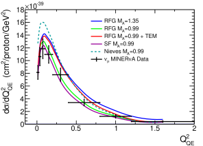
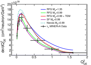
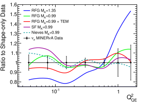
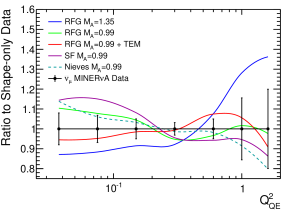
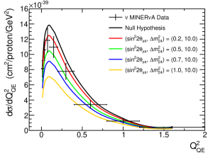
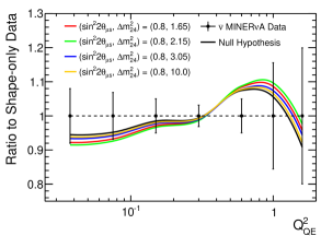
Unbiased cross-section predictions corresponding to the null hypothesis are shown for each cross-section model in Figure 1. The effect of sterile neutrino induced biases on the RFG + TEM model over a range of mixing parameters can be seen in Figure 2. Changes in $E_{\nu}$ distributions introduced by the bias have only a small effect on the shape because the peak neutrino energy is higher than the experimental kinematic limit $2m_{p}E_{\nu}>Q^{2}$ mcfarland11 . The shape’s response to sterile modifications is likely to be larger for other experiments.

Figure 1: Neutrino (left) and antineutrino (right) flux-averaged cross-section predictions are shown for all cross-section models investigated without any sterile neutrino bias. The upper panel shows the differential cross-section and the lower panel the ratio of model to data. In the ratio model and data are area normalised. The error bars on the MINER$\nu$A data include both statistical and systematic errors.

Figure 2: Example sterile hypotheses for the RFG+TEM antineutrino model. Ratio to shape-only data (area normalised to unity) is shown to highlight the limited shape sensitivity to sterile modifications.

The initial $\chi^{2}$ definition used to fit the sterile hypotheses to data is

$$\chi^{2}=\sum_{i=1}^{16}\sum_{j=1}^{16}\left(\nu_{i}^{M}-\nu_{i}^{D}\right)M_{ij}^{-1}\left(\nu_{j}^{M}-\nu_{j}^{D}\right)\,,$$ (6)

where $M_{ij}$ is the covariance matrix, $\nu_{i}^{D}$ are the measured differential cross-section in $Q^{2}_{QE}$ bins, and $\nu_{j}^{M}$ are calculated using Equation (5). It was found that minimizing this statistic gave results far below the data points, an effect consistent with “Peelle’s Pertinent Puzzle” (PPP) peelle87puzzle .

PPP can occur when fitting to a dataset containing large correlated uncertainties between all bins. If the total normalisation is reduced in the fit, the relative size of the shape errors increases, thus appearing to improve the agreement even if the shape of the prediction has not changed peelle87puzzle . This causes the fit to prefer parameter values which predict a distribution that lies far below the data carlson09peelle . We avoid the PPP problem by separating the MINER$\nu$A covariance matrix into a total normalisation error, $\epsilon=10.9\%$, and a shape-only matrix, $M_{ij}^{shape}$ agostini94covar .

The extracted shape-only covariance matrix, $M_{ij}^{shape}$, could not be inverted analytically as a result of rounding errors in the published MINER$\nu$A data. We dealt with this problem by using the two-step method of ref cteq01parton , in which the bin errors and correlations are treated separately. The alternative $\chi^{2}$ definition is given by

$$\chi^{2}=\left[\sum_{i=1}^{16}\left(\frac{\nu_{i}^{D}-(\nu_{i}^{M}/\alpha)}{\sigma_{i}}\right)^{2}-\sum_{i=1}^{16}\sum_{j=1}^{16}C_{i}(A^{-1})_{ij}C_{j}\right]+\left(\frac{1-\alpha}{\epsilon}\right)^{2}\,,$$ (7)

where $\sigma_{i}$ are the uncorrelated shape-only statistical errors for the dataset. The shape-only correlated uncertainties are contained in $C_{i}(A^{-1})_{ij}C_{j}$ which is defined in Appendix A. The advantage of this procedure is that $A_{ij}$ is an invertible matrix. The constrained parameter $\alpha$ normalised the theoretical predictions to the total measured cross-section in the experimental range, allowing the square bracket to represent shape-only contributions while the final penalty term reflected the difference in normalisation between the MC and data. The combination of these techniques was found to be a robust way to fit a highly correlated dataset affected by PPP (for a more detailed explanation of PPP and the definition of (7), see Appendix A).

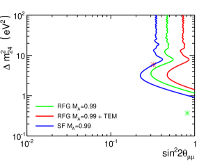
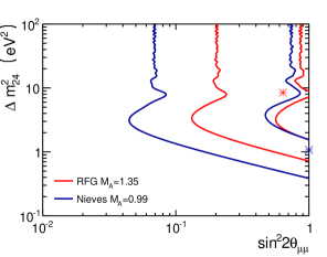
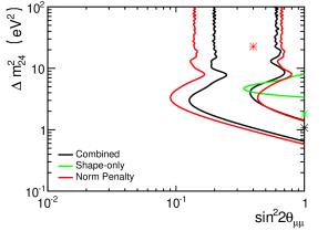
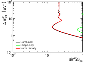
For each cross-section model, parameter scans were performed for values in the ranges 0.0 $\leq\sin^{2}2\theta_{\mu\mu}\leq$ 1.0 over 500 evenly spaced bins and $\mbox{0.1 eV}^{2}/\mbox{c}^{4}\leq\Delta m_{24}^{2}\leq\mbox{100 eV}^{2}/\mbox{c}^{4}$ over 1000 logarithmic bins. For each parameter bin a sterile bias was introduced using the bin centre co-ordinates and a $\chi^{2}$ value calculated using Equation (7). The minimum $\chi^{2}$ values from the scans were passed as starting assumptions to MINUIT which then found a true $\chi^{2}$ minimum in the parameter space minuit75 ; brun97root . Best fit points and minimum $\chi^{2}$ values for each model can be found in Table 2. A $\Delta\chi^{2}$ method was used to produce 90% CL confidence limits around the best fit points as shown for all cross-section models in Figure 3. The $1\sigma$ confidence limits for the separate shape-only or normalisation penalty terms from Equation (7) are compared in Figure 4 for the Nieves and SF models to highlight the relative strength of the normalisation term.

Model	RFG 1.35	RFG 0.99	TEM 0.99	SF 0.99	NEV 0.99
Nucleon distribution	RFG	RFG	RFG	SF	LFG
$M_{\mathrm{A}}$ (GeV/c2)	1.35	0.99	0.99	0.99	0.99
Enhancements	-	-	TEM	-	Nieves + RPA
Null $\chi^{2}/15$	2.332	2.433	1.663	2.833	2.971
Best sterile $\chi^{2}/13$	1.803	2.803	1.628	3.253	2.943
Best $\sin^{2}2\theta_{\mu\mu}$	0.638	0.817	0.322	0.000	1.000
Best $\Delta m^{2}_{24}$ (eV2)	8.463	0.370	5.913	0.104	1.073

Table 2: Null hypothesis and best fit sterile hypothesis $\chi^{2}/Ndof$ values.

Figure 3: 90% CL mixing parameter contours and best fit points (starred) for the cross-section models investigated.

Figure 4: Overlaid shape-only, normalisation-only, and combined contours at the $1\sigma$ confidence limit. The Nieves (left) and SF (right) models are shown. Best fit points are indicated by a star.

6 Discussion and conclusion

The $\chi^{2}$ values in Table 2 and the contours in figures 3 and 4 demonstrate the sensitivity of sterile neutrino fits to the adopted cross-section model. Some models, e.g. RFG 1.35, exclude the null hypothesis at >99%CL, while others, e.g. SF 0.99, prefer it. The choice of axial mass value is a critical parameter (compare RFG 1.35 with RFG 0.99), but other features of the models tested also have significant effects (consider RFG 0.99 and TEM 0.99). It is clear that in many situations the choice of cross-section model can completely dominate the results obtained in sterile neutrino searches.

In the case of the MINER$\nu$A dataset considered in this study, the weakness of the final limits can be attributed to the large normalisation error. It is worth noting that the magnitude of the disagreement between models is likely to increase when analysing data with a smaller normalisation error or a stronger shape response to sterile neutrino biases. We conclude that sterile mixing limits obtained in this way are subject to large systematic uncertainties, until they can be repeated with a well-motivated theoretical model that agrees well with existing neutrino data.

Appendix A $\chi^{2}$ definition and fake data study

There is a well documented problem that can arise when fitting data with a covariance matrix that contains large correlated uncertainties between bins, as in Equation (8) agostini94covar . By suppressing the normalisation of the prediction the $\chi^{2}$ is reduced, leading to a best fit distribution well below the data. This occurs because the covariance matrix is evaluated at a single point and the shape-only errors do not scale with normalisation. This problem is known as “Peelle’s Pertinent Puzzle” (PPP) peelle87puzzle .

$$\chi^{2}=\sum_{i=1}^{16}\sum_{j=1}^{16}\left(\nu_{i}^{M}-\nu_{i}^{D}\right)M_{ij}^{-1}\left(\nu_{j}^{M}-\nu_{j}^{D}\right)$$ (8)

Protecting against PPP is particularly important for sterile neutrino analyses, where a signal would involve a suppression of the overall normalisation, and a large normalisation uncertainty due to uncertainties in the flux prediction is common for accelerator experiments. PPP can be overcome by redefining the $\chi^{2}$ in terms of the shape-only matrix, $M_{ij}^{shape}$, and scaling the total integrated MC cross-section to match the total integrated cross-section in the data. This definition effectively stops the fit from inflating the relative size of the shape-only errors agostini94covar .

$$\chi^{2}=\sum_{i=1}^{16}\sum_{j=1}^{16}\left(\nu_{i}^{M}-\nu_{i}^{D}\right)\left(M_{shape}^{-1}\right)_{ij}\left(\nu_{j}^{M}-\nu_{j}^{D}\right)$$ (9)

We obtain $M_{ij}^{shape}$ and the total normalisation uncertainty $\epsilon$ from the published matrix $M_{ij}$ using the MiniBooNE matrix seperation method reproduced in Equation (10) teppei08extract .

$$\nu_{T} =\sum_{k}^{16}\nu_{k}^{D}\,,\quad\quad\alpha=\frac{\sum_{i}^{16}\nu_{i}^{M}}{\nu_{T}}\,,$$

$$\epsilon =\frac{1}{\nu_{T}}\sqrt{M_{ij}^{norm}}=\frac{1}{\nu_{T}}\sqrt{\sum_{k}^{16}\sum_{l}^{16}M_{kl}}\,,$$

$$M_{ij}^{shape} =M_{ij}-\frac{\nu^{D}_{i}}{\nu_{T}}\sum_{k}^{16}M_{kj}-\frac{\nu^{D}_{j}}{\nu_{T}}\sum_{k}^{16}M_{ik}+\frac{\nu^{D}_{i}\nu^{D}_{j}}{\nu_{T}^{2}}\sum_{k}^{16}\sum_{l}^{16}M_{kl}\,.$$ (10)

The matrix separation method involves summations over many matrix elements which can lead to large rounding errors in $M_{ij}^{shape}$ if $M_{ij}$ is given to limited precision, as is the case for the MINER$\nu$A data release. This can cause problems when inverting $M_{ij}^{shape}$. We modify the $\chi^{2}$ definition in Equation (9) to avoid inverting the matrix $M_{ij}^{shape}$ using the method given in ref. cteq01parton . The final $\chi^{2}$ definition used in our fits is given by

$$\chi^{2}=\left[\sum_{i=1}^{16}\left(\frac{\nu_{i}^{D}-(\nu_{i}^{M}/\alpha)}{\sigma_{i}}\right)^{2}-\sum_{i=1}^{16}\sum_{j=1}^{16}C_{i}(A^{-1})_{ij}C_{j}\right]+\left(\frac{1-\alpha}{\epsilon}\right)^{2}\,,$$ (11)

where $\sigma_{i}$ is the uncorrelated shape-only statistical error on the $i^{th}$ bin, and $\Delta_{ik}$ is the correlated shape-only systematic uncertainty between the $i^{th}$ and $k^{th}$ bins which can be calculated using $\sum_{k=1}^{16}\Delta_{ik}\Delta_{kj}=M_{ij}^{shape}-\sigma^{2}_{i}\delta_{ij}$. The vector $C$ and matrix $A$ are defined by

$$C_{i}=\sum_{k=1}^{16}\frac{\Delta_{ik}(\nu^{D}_{i}-(\nu^{M}_{i}/\alpha))}{\sigma_{k}^{2}}\,,\quad\quad A_{ij}=\delta_{ij}+\sum_{k=1}^{16}\frac{\Delta_{ik}\Delta_{jk}}{\sigma_{k}^{2}}\,.$$ (12)

The matrix $A$, which is inverted in this method, is less susceptible to the rounding error problems than the full matrix $M_{ij}^{shape}$. Note that with more complete information the matrix $A$ can be reduced to a $N\times N$ matrix for $N$ systematic errors as described in ref. cteq01parton .

To test the $\chi^{2}$ statistic as a method of fitting for sterile induced biases, we conducted a fake data study using the RFG 1.35 dataset. We generated 30 sets of sterile parameters and generated fake data for each using the following method.

First, MC was generated with the given parameter values according to the method described in Section 5. Then the systematic covariance matrix was calculated from the MINER$\nu$A matrix, $M_{ij}$, and added to a diagonal matrix representing the statistical variance for the fake data study to create a fake data covariance matrix, $M_{ij}^{F}$, as shown in Equation (13). This covariance matrix would have been produced if the fake data reflected nature, and was measured in the MINER$\nu$A detector.

$$M^{F}_{ij} =\frac{\nu^{M}_{i}\nu^{M}_{j}}{\nu^{D}_{i}\nu^{D}_{j}}\left[M_{ij}-\delta_{ij}\left((\sigma^{D})_{i}^{2}-(\sigma^{MC})_{i}^{2}\right)\right]$$ (13)

Throwing the matrix using the Cholesky decomposition method and adding the result to the nominal fake data produces a realistic fake data sample efron1994introduction . The residuals from 2000 throws were calculated and fitted with a Gaussian to look for biases for each of the 30 sterile parameter sets investigated. These were found to have pulls away from the true parameter in the range of $-0.05$ to $0.10$ for $\sin^{2}2\theta_{\mu\mu}$ and $-0.24$ to $0.28$ for $\Delta m^{2}_{24}$, and widths in the range of $0.81$ to $0.98$ for $\sin^{2}2\theta_{\mu\mu}$ and $0.75$ to $0.98$ for $\Delta m^{2}_{24}$. It was concluded that the $\chi^{2}$ statistic is a good estimator of the central value and was appropriate for the analysis.