Interfacial Cracks in Piezoelectric Bimaterials:
an approach based on Weight Functions and
Boundary Integral Equations

Abstract

The focus of this paper is on the analysis of a semi-infinite crack lying along a perfect interface in a piezoelectric bimaterial with arbitrary loading on the crack faces. Making use of the extended Stroh formalism for piezoelectric materials combined with Riemann-Hilbert formulation, general expressions are obtained for both symmetric and skew-symmetric weight functions associate with plane crack problems at the interface between dissimilar anisotropic piezoelectric media. The effect of the coupled electrical fields is incorporated in the derived original expressions for the weight function matrices. These matrices are used together with Betti’s reciprocity identity in order to obtain singular integral equations relating the extended displacement and traction fields to the loading acting on the crack faces. In order to study the variation of the piezoelectric effect, two different poling directions are considered. Examples are shown for both poling directions with a number of mechanical and electrical loadings applied to the crack faces.

Keywords: Interfacial crack, Piezoelectric bimaterial, Weight function, Betti’s identity, Singular integral equations.

1 Introduction

Fracture in piezoelectric materials is an area of great interest due to their many applications in industry, for example, in piezoelectric insulators and actuators [1, 2]. The problem of a static semi-infinite interfacial crack between dissimilar anisotropic piezoelectric materials under symmetric loading conditions has been studied in Suo et al. [3] using an approach based on the Stroh formalism [4] and Riemann-Hilbert formulation. As an alternative to this method, singular integral formulations for two-dimensional interfacial crack problems in piezoelectric bimaterials have been derived by means of approaches based on Green’s function method [5]. Applying this procedure, the displacements and the stresses are defined by integral relations involving the Green’s functions, for which explicit expressions are required. Although Green’s functions for several crack problems in piezoelectric bimaterials have been derived [6, 7], their utilisation in evaluating physical displacements and stress fields on the crack faces requires challenging numerical estimation of integrals for which convergence should be asserted carefully. Moreover, both the complex variable formulation proposed by Suo et al. [3] and the approaches based on Green’s function method work when the tractions applied on the discontinuity surface are symmetric, but not in the case of asymmetric loading acting on the crack faces.

In this paper, we illustrate a general procedure for studying plane interfacial crack problems in anisotropic piezoelectric bimaterials in the presence of a general non-symmetric mechanical and electrostatic loading distribution acting on the crack faces. The approach developed in Piccolroaz et al. [8] and Piccolroaz and Mishuris [9], based on weight function theory and Betti’s reciprocity theorem, is extended to the case of an interfacial crack in a piezoelectric bimaterial containing a perfect interface. Applying this method, the crack problem is also formulated in terms of singular integral equations avoiding the use of Green’s functions and the resulting challenging computations.

In fracture mechanics the notion of weight function, defined as the stress intensity factor associated to a point load acting on the crack faces, was originally introduced by Bueckner [10, 11, 12] and Rice [13]. This weight functions concept have been extended for studying crack problems in piezoelectric materials by McMeeking and Ricoeur [14] and Ma and Chen [15]. An alternative formulation where the weight functions are defined as the singular displacement field of the homogeneous traction free problem was proposed by Willis and Movchan [16]. Recently, this weight functions definition has been used in the derivation of stress intensity factors for both static and dynamic crack problems in isotropic and anisotropic bimaterials [8, 17, 18] and in thermodiffusive elastic media [19]. These weight functions have also been used in the derivation of singular integral equations relating interfacial tractions and crack displacement to the applied loadings on the crack faces [9, 20, 21]. In this paper, this method is generalised in order to study interfacial cracks in piezoelectric bimaterials. Explicit weight functions are derived for the class of transversely isotropic piezoelectric bimaterials considering two different poling directions [22]. Then these weight function matrices are used together with the generalised Betti’s identity to derive singular integral equations relating the tractions and displacements to the electric fields introduced by the piezoelectric effect. Finally, some simple illustrative examples of the application of the obtained singular integral identities are reported.

Section 2 of the paper introduces the problem geometry and a number of preliminary results required for further analysis. In Section 3 we derive weight functions for transversely isotropic piezoelectric bimaterials considering two different poling directions using the definition introduced by Willis and Movchan [16]. The problem is reduced to only contain the fields affected by the piezoelectric effect. In Section 4 the obtained weight function matrices are used together with Betti’s identity in order to derive singular integral equations relating the physical fields to the applied mechanical and electrical loadings on the crack faces. In Section 5 we present a number of examples for a variety of mechanical and electrical loadings. For one of the considered examples we also present the results from finite element computations and compare their accuracy to those obtained from our singular integral equations.

2 Problem formulation and preliminary results

In this section we introduce the mathematical model used for the remainder of the paper. Some preliminary results concerning two-dimensional interfacial cracks in anisotropic piezoelectric bimaterials are reported.

We consider a semi-infinite crack lying along a perfect interface between two dissimilar piezoelectric half-planes, referred to as materials I and II. The crack occupies the region $\{x_{1}<0,x_{2}=0\}$, as illustrated in Figure 1. The perfect interface conditions in a piezoelectric bimaterial are continuity of displacements, traction, electric potential and the electric charge. The loading along the crack faces, for $x_{1}<0$, is known and given by the functions

$$p_{j}^{\pm}(x_{1})=\sigma_{2j}(x_{1},0^{\pm}),\quad\text{for }j=1,2,3,\quad p_{4}^{\pm}(x_{1})=D_{2}(x_{1},0^{\pm}),$$ (1)

where $\sigma_{ij}$ and ${D_{i}}$ represent tractions and electrical displacements respectively.

Expressions for the stress fields and displacements for a plane semi-infinite interfacial crack between dissimilar piezoelectric media have been derived by Suo et al. [3], using an approach based on Stroh formalism [4] and Riemann-Hilbert formulation. This method, which is applied in the paper in order to derive explicit weight functions for piezoelectric bimaterials, is summarised in Section 2.1.

In Section 2.2, the definition of weight functions proposed in Piccolroaz et al. [23] and Morini et al. [17] is extended to the case of interfacial cracks between dissimilar piezoelectric materials. Finally, in Section 2.3, the expression for the Betti’s formula generalized to piezoelectric media by Hadjesfandiari [24] is reported. Further in the text, weight functions and Betti’s formula are used for formulating the crack problem shown in Fig. 1 in terms of singular integral equations.

Figure 1: A semi-infinite crack along an interface between two dissimilar piezoelectric materials subject to the state of generalised plane strain and short circuit $(\varepsilon_{3}^{\pm}=E_{3}^{\pm}=0)$

2.1 Stroh formalism for piezoelectric materials

Under the conditions of static deformations, the governing equations for a linear and generally anisotropic piezoelectric body are [25, 26]:

$$\sigma_{ij,i}=0,\qquad D_{i,i}=0,$$ (2)

where body forces are assumed to be zero. The strain $\epsilon$ and electric field $\mathbf{E}$, are defined by the gradients

$$\varepsilon_{ij}=\frac{1}{2}(u_{i,j}+u_{j,i}),\qquad E_{i}=-\phi_{,i},$$ (3)

where $u_{i}$ are the components of the displacement field and $\phi$ is the electric potential.

The constitutive relations for anisotropic piezoelectric materials are given by Wang and Zhou [27]

$$\sigma_{ij}=C_{ijrs}\varepsilon_{rs}-e_{sji}E_{s},\qquad D_{i}=\omega_{is}E_{s}+e_{irs}\varepsilon_{rs},$$ (4)

where the tensors $C$, $\omega$ and $e$ represent the stiffness, permittivity and piezoelectricity respectively. Combining equations (2), (3) and (4) the following relationships are obtained

$$(C_{ijrs}u_{r}+e_{sji}\phi)_{,si}=0,\qquad(-\omega_{is}\phi+e_{irs}u_{r})_{,si}=0.$$ (5)

Considering the semi-infinite interfacial crack problem shown in Fig. 1, and assuming for both the upper and lower piezoelectric half-planes the state of generalised plane strain and short circuit $(\varepsilon_{3}=0$ and $E_{3}=0)$, a solution for equations (5) is derived by applying the procedure described by Suo et al. [3]. The solution is sought in the form $(u_{r},\phi)^{T}=\mathbf{a}f(z)$ where $z=x_{1}+px_{2}$. This yields the following eigenvalue problem

$$[\mathbf{Q}+p(\mathbf{R}+\mathbf{R}^{T})+p^{2}\mathbf{T}]\mathbf{A}=0$$ (6)

For general, anisotropic piezoelectric media the matrices have the following form:

$$\mathbf{Q}=\begin{pmatrix}C_{11}&C_{16}&C_{15}&e_{11}\\ C_{16}&C_{66}&C_{56}&e_{16}\\ C_{15}&C_{56}&C_{55}&e_{15}\\ e_{11}&e_{16}&e_{15}&-\omega_{11}\end{pmatrix},\quad\mathbf{R}=\begin{pmatrix}C_{16}&C_{12}&C_{14}&e_{16}\\ C_{66}&C_{26}&C_{46}&e_{12}\\ C_{56}&C_{25}&C_{45}&e_{14}\\ e_{21}&e_{26}&e_{25}&-\omega_{12}\end{pmatrix},\quad\mathbf{T}=\begin{pmatrix}C_{66}&C_{26}&C_{46}&e_{26}\\ C_{26}&C_{22}&C_{24}&e_{22}\\ C_{46}&C_{24}&C_{44}&e_{24}\\ e_{26}&e_{22}&e_{24}&-\omega_{22}\end{pmatrix}.$$

The eight eigenvalues of (6) are found to be four pairs of complex conjugate

For the remainder of this paper $\mathbf{u}$ shall be used to the extended vector containing both the physical displacement and electric potential given by $\mathbf{u}=(u_{1},u_{2},u_{3},\phi)^{T}$. The extended traction vector, $\mathbf{t}$, is also introduced, given by $\mathbf{t}=(\sigma_{2i},D_{2})^{T}$. It was shown in Suo et al. [3] that the extended displacements and traction are given by

$$\mathbf{u}=2\mathrm{Re}\sum_{\mu=1}^{4}\mathbf{A}_{\mu}f_{\mu}(z_{\mu}),\qquad\mathbf{t}=2\mathrm{Re}\sum_{\mu=1}^{4}\mathbf{L}_{\mu}f^{\prime}_{\mu}(z_{\mu}).$$ (7)

where

$$L_{j\mu}=\sum_{r=1}^{3}[(C_{2jr1}+p_{\mu}C_{2jr2})A_{r\mu}]+(e_{1j2}+p_{\mu}e_{2j2})A_{4\mu},\quad\text{for }j=1,2,3,$$

$$L_{4\mu}=\sum_{r=1}^{3}[(e_{2r1}+p_{\mu}e_{2r2})A_{r\mu}]-(\omega_{12}+p_{\mu}\omega_{22})A_{4\mu}.$$

The values of $z_{\mu}$ are given by $z_{\mu}=x_{1}+p_{\mu}x_{2}$, where the eigenvalues, $p_{\mu}$, are taken to be those with positive imaginary part and the matrix $\mathbf{A}_{\mu}$ are the corresponding eigenvectors. The surface admittance tensor $\mathbf{B}=i\mathbf{AL}^{-1}$ is introduced and for further analysis the following bimaterial matrices are defined

$$\mathbf{H}=\mathbf{B}_{I}+\bar{\mathbf{B}_{II}},\qquad\mathbf{W}=\mathbf{B}_{I}-\bar{\mathbf{B}_{II}}.$$ (8)

Assuming vanishing tractions and electrical displacement along the crack faces for $x_{1}<0$, and using expressions (7), in Suo et al. [3] the following Riemann-Hilbert problem was found to exist along the negative $x_{1}$- axis

$$\mathbf{h}^{+}(x_{1})+\bar{\mathbf{H}}^{-1}\mathbf{H}\mathbf{h}^{-}(x_{1})=0,\quad-\infty<x_{1}<0.$$ (9)

A solution is found in the form $\mathbf{h}(z)=\mathbf{w}z^{-\frac{1}{2}+i\epsilon}$ where the branch cut is situated along the negative real axis (which is the crack line). Inserting this solution into equation (9) yields the eigenvalue problem

$$\bar{\mathbf{H}}\mathbf{w}=e^{2\pi\epsilon}\mathbf{H}\mathbf{w}.$$ (10)

Four pairs of eigenvectors and eigenvalues are found from (10). They are

$$(\epsilon,\mathbf{w}),\>(-\epsilon,\bar{\mathbf{w}}),\>(-i\kappa,\mathbf{w}_{3}),\>(i\kappa,\mathbf{w}_{4}).$$ (11)

Imposing the continuity of tractions and electrical displacement along the interface ahead of the crack tip, the following formula for determining the extended traction vector $\mathbf{t}$ is derived [3]:

$$\mathbf{h}^{+}(x_{1})+\bar{\mathbf{H}}^{-1}\mathbf{H}\mathbf{h}^{-}(x_{1})=\mathbf{t}(x_{1}),\quad 0<x_{1}<\infty.$$ (12)

The extended traction vector, derived by means of equation (12), is therefore given by

$$\mathbf{t}(x_{1})=(2\pi x_{1})^{-\frac{1}{2}}[Kx_{1}^{i\epsilon}\mathbf{w}+\bar{K}x_{1}^{-i\epsilon}\bar{\mathbf{w}}+K_{3}x_{1}^{\kappa}\mathbf{w}_{3}+K_{4}x_{1}^{-\kappa}\mathbf{w}_{4}],$$ (13)

where $K=K_{1}+iK_{2}$. The stress intensity factor vector is given by $\mathbf{K}=(K,\bar{K},K_{3},K_{4})^{T}$.

The extended displacement jump across the crack, given by $\llbracket\mathbf{u}\rrbracket(x_{1})=\mathbf{u}^{+}(x_{1})-\mathbf{u}^{-}(x_{1})$, was found to be

$$\llbracket\mathbf{u}\rrbracket(x_{1})=(\mathbf{H}+\bar{\mathbf{H}})\sqrt{\frac{(-x_{1})}{2\pi}}\bigg{[}\frac{K(-x_{1})^{i\epsilon}\mathbf{w}}{(1+2i\epsilon)\cosh\pi\epsilon} +\frac{\bar{K}(-x_{1})^{-i\epsilon}\bar{\mathbf{w}}}{(1-2i\epsilon)\cosh\pi\epsilon}$$

$$+\frac{K_{3}(-x_{1})^{\kappa}\mathbf{w}_{3}}{(1+2\kappa)\cos\pi\kappa}+\frac{K_{4}(-x_{1})^{-\kappa}\mathbf{w}_{4}}{(1-2\kappa)\cos\pi\kappa}\bigg{]}.$$ (14)

Using these expressions for the traction and displacement jump the following equation can be used to find the energy release rate at the crack tip

$$G=\frac{1}{2\nu}\int_{0}^{\nu}\mathbf{t}^{T}(\Delta-r)[\mathbf{u}](r)\mathrm{d}r,$$ (15)

for an arbitrary value of $\nu$. Using expressions (13) and (2.1) it can be shown that

$$G=\frac{\bar{\mathbf{w}}^{T}(\mathbf{H}+\bar{\mathbf{H}})\mathbf{w}}{4\cosh^{2}\pi\epsilon}|K|^{2}+\frac{\mathbf{w}_{3}^{T}(\mathbf{H}+\bar{\mathbf{H}})\mathbf{w}_{4}}{4\cos^{2}\pi\kappa}K_{3}K_{4}.$$ (16)

2.2 Weight functions for piezoelectric bimaterials: definition

Weight functions, introduced in Bueckner [11, 12], are functions whose weighted integrals can be used in the derivation of important fracture parameters, such as the stress intensity factors. For elastic materials Willis and Movchan [16] introduced a weight function given by the singular displacement field corresponding to a homogeneous, traction-free problem similar to Fig. 1 with the crack occupying the region $x_{1}>0$ and the perfect interface lying along the region $x_{1}<0$. This concept of a weight function has been adopted in the works of Piccolroaz et al. [23] and Morini et al. [17] for studying interfacial cracks in isotropic and anisotropic bimaterials, respectively. Here, this approach is extended to piezoelectric materials.

The weight function for piezoelectric materials is given by the extended singular displacement field $\mathbf{U}$ incorporating both displacement and electric potential. The symmetric and skew-symmetric parts of the weight function across the plane $x_{2}=0$ are given by

$$\llbracket\mathbf{U}\rrbracket(x_{1})=\mathbf{U}(x_{1},0^{+})-\mathbf{U}(x_{1},0^{-}),$$ (17)

$$\langle\mathbf{U}\rangle(x_{1})=\frac{1}{2}\left[\mathbf{U}(x_{1},0^{+})+\mathbf{U}(x_{1},0^{-})\right].$$ (18)

To satisfy the perfect interface conditions it is clear that $\llbracket\mathbf{U}\rrbracket=0$ for $x_{1}<0$.

The extended traction field corresponding to the extended displacement $\mathbf{U}$, is denoted $\mathbf{\Sigma}$. The following Riemann-Hilbert problem is found along the positive portion of the $x_{1}$-axis

$$\mathbf{h}^{+}(x_{1})+\bar{\mathbf{H}}^{-1}\mathbf{H}\mathbf{h}^{-}(x)=0,\quad 0<x_{1}<\infty.$$ (19)

A solution for $\mathbf{h}(z)$ is now sought in the form $\mathbf{h}=\mathbf{v}^{-\frac{3}{2}+i\epsilon}$. The branch cut of $\mathbf{h}$ is situated along the positive part of the $x_{1}$axis. Inserting this solution into (19) yields the following eigenvalue problem

$$\bar{\mathbf{H}}\mathbf{v}=e^{-2\pi\epsilon}\mathbf{H}\mathbf{v}.$$ (20)

It is immediately clear by comparing equation (10) to (20) that $\mathbf{v}=\bar{\mathbf{w}}$, $\mathbf{v}_{3}=\mathbf{w}_{4}$ and $\mathbf{v}_{4}=\mathbf{w}_{3}$.

Along the negative part of the real axis $\mathbf{\Sigma}$ is given by

$$\mathbf{h}^{+}(x_{1})+\bar{\mathbf{H}}^{-1}\mathbf{H}\mathbf{h}^{-}(x)=\mathbf{\Sigma}(x_{1}),\quad-\infty<x_{1}<0.$$ (21)

Therefore the extended traction vector corresponding to the weight function $\mathbf{U}$ is given by

$$\mathbf{\Sigma}(x_{1})=\frac{(-x_{1})^{-3/2}}{2\sqrt{2\pi}}\left[C(-x_{1})^{i\epsilon}\bar{\mathbf{w}}+\bar{C}(-x_{1})^{-i\epsilon}\mathbf{w}+C_{3}(-x_{1})^{-\kappa}\mathbf{w}_{3}+C_{4}(-x_{1})^{\kappa}\mathbf{w}_{4}\right],$$ (22)

where $C=C_{1}+iC_{2}$, $C_{3}$ and $C_{4}$ are constants defined in the same manner as the stress intensity factors for the physical problem.

Let us introduce the Fourier transform of a generic function $f$ with respect to the variable $x_{1}$, defined as follows:

$$\hat{f}(\xi)=\mathcal{F}[f(x_{1})]=\int_{-\infty}^{+\infty}f(x_{1})e^{i\xi x_{1}}dx_{1},\quad f(x_{1})=\mathcal{F}^{-1}[\hat{f}(\xi)]=\frac{1}{2\pi}\int_{-\infty}^{+\infty}\hat{f}(\xi)e^{-i\xi x_{1}}d\xi.$$ (23)

For anisotropic materials it was shown in Morini et al. [17] that the Fourier transforms of the symmetric and skew-symmetric parts of the weight functions are related to $\hat{\Sigma}$ in the following manner

$$\llbracket\hat{\mathbf{U}}\rrbracket^{+}(\xi)=\frac{1}{|\xi|}(i\mathrm{sign}(\xi)\mathrm{Im}(\mathbf{H})-\mathrm{Re}(\mathbf{H}))\hat{\Sigma}^{-}(\xi),$$ (24)

$$\langle\hat{\mathbf{U}}\rangle(\xi)=\frac{1}{2|\xi|}(i\mathrm{sign}(\xi)\mathrm{Im}(\mathbf{W})-\mathrm{Re}(\mathbf{W}))\hat{\Sigma}^{-}(\xi),$$ (25)

As the method used in Morini et al. [17] was for general matrices $\mathbf{H}$ and $\mathbf{W}$, it is immediately clear that these results also hold for piezoelectric materials.

2.3 The generalised Betti formula

In this part of the paper we consider the Betti identity in the context of a semi-infinite crack in a piezoelectric bimaterial. Originally used to relate two different sets of displacement and traction fields satisfying the equilibrium equations [16, 23], this approach was extended to study piezoelectric materials (with electric potential and electric displacement) by Hadjesfandiari [24]. The derivation of Betti formula for piezoelectric solids is briefly reported in Appendix A. This integral formula is now used to form a relationship between the physical fields and the weight function introduced in the previous part of the paper.

Applying the generalised Betti formula derived in Hadjesfandiari [24] to the semi-circular domain occupying the upper half plane in the model illustrated in Fig. 1, the following integral relation is found

$$\int_{x_{2}=0^{+}}\left[\mathbf{R}\mathbf{U}(x_{1}^{\prime}-x_{1},0^{+})\cdot\mathbf{t}(x_{1},0^{+})-\mathbf{R}\mathbf{\Sigma}(x_{1}^{\prime}-x_{1},0^{+})\cdot\mathbf{u}(x_{1},0^{+})\right]\mathrm{d}x_{1}=0,$$ (26)

where $\mathbf{u}=(u_{1},u_{2},u_{3},\phi)^{T}$ and $\mathbf{t}=(\sigma_{21},\sigma_{22},\sigma_{23},D_{2})^{T}$ (see the Appendix for details) and $\mathbf{R}$ is given by

$$\mathbf{R}=\begin{pmatrix}-1&0&0&0\\ 0&1&0&0\\ 0&0&-1&0\\ 0&0&0&-1\end{pmatrix}.$$

The equivalent equation for a semi-circular domain in the lower half-plane gives

$$\int_{x_{2}=0^{-}}\left[\mathbf{R}\mathbf{U}(x_{1}^{\prime}-x_{1},0^{-})\cdot\mathbf{t}(x_{1},0^{-})-\mathbf{R}\mathbf{\Sigma}(x_{1}^{\prime}-x_{1},0^{-})\cdot\mathbf{u}(x_{1},0^{-})\right]\mathrm{d}x_{1}=0.$$ (27)

Subtracting equation (27) from (26) yields the following relationship

$$\mathbf{R}\llbracket\mathbf{U}\rrbracket\ast\mathbf{t}^{(+)}-\mathbf{R}\mathbf{\Sigma}^{(-)}\ast\llbracket\mathbf{u}\rrbracket=-\mathbf{R}\llbracket\mathbf{U}\rrbracket\ast\langle\mathbf{p}\rangle-\mathbf{R}\langle\mathbf{U}\rangle\ast\llbracket\mathbf{p}\rrbracket,$$ (28)

where $\ast$ represents the convolution with respect to $x_{1}$ and ^(±) is used to represent the restriction of a function to the positive or negative portion of the $x_{1}$-axis respectively. It can be easily deduced that in equation (28) the contribution to the generalised traction vector defined on the negative semi-axis $x_{1}<0$ is given by the loading functions $\mathbf{t}^{(-)}=(\sigma_{21}^{(-)},\sigma_{22}^{(-)},\sigma_{23}^{(-)},D_{2}^{(-)})^{T}=(p_{1},p_{2},p_{3},p_{4})^{T}=\mathbf{p}$, and the symmetrical and skew-symmetrical part of the load, respectively $\langle\mathbf{p}\rangle$ and $\llbracket\mathbf{p}\rrbracket$, are defined as follows [9]:

$$\langle\mathbf{p}\rangle=\frac{1}{2}(\mathbf{p}^{+}+\mathbf{p}^{-}),\quad\llbracket\mathbf{p}\rrbracket=\mathbf{p}^{+}-\mathbf{p}^{-}.$$ (29)

Applying the Fourier transform to (28) gives the following relationship

$$\llbracket\hat{\mathbf{U}}\rrbracket^{T}\mathbf{R}\hat{\mathbf{t}}^{+}-(\hat{\mathbf{\Sigma}}^{-})^{T}\mathbf{R}\llbracket\hat{\mathbf{u}}\rrbracket=-\llbracket\hat{\mathbf{U}}\rrbracket^{T}\mathbf{R}\langle\hat{\mathbf{p}}\rangle-\langle\hat{\mathbf{U}}\rangle^{T}\mathbf{R}\llbracket\hat{\mathbf{p}}\rrbracket.$$ (30)

In the next Sections, explicit expressions for the weight function matrices (24) and (25) are derived and used together with the the generalised Betti identity (30) for formulating the considered interface crack problem in terms of singular integral equations. Since the bimaterial matrices $\mathbf{H}$ and $\mathbf{W}$ involved in the weight functions (24) and (25) depend on the surface admittance tensors of both piezoelectric half-planes (see definition (8)), in order to derive explicit expressions for these matrices the solution of the Stroh’s eigenvalue problem (6) is needed. In the general fully anisotropic case, this eigenvalue problem must be solved numerically. Nevertheless, exact algebraic expressions of Stroh’s eigenvalues and eigenvectors have been obtained for the class of transversely isotropic piezoelectric materials in [3, 22, 28] and [29]. This class of materials has practical significance, because many poled ceramics that are actually in use fall into this category. The Stroh matrices and surface admittance tensors for transversely isotropic piezoelectric materials with poling direction parallel to $x_{2}$ and $x_{3}$ axes are reported in the Appendix. Further in the text, these results will be used together with expressions (24) and (25) for deriving explicit weight function matrices corresponding to interfacial cracks between dissimilar transversely isotropic piezoceramics.

3 Weight functions

Piezoelectric materials occupying both lower and upper half-planes in Figure 1 are assumed to be transversely isotropic. For simplicity, poling direction is assumed to be parallel to the $x_{2}$ and $x_{3}$ axes, respectively. Using eigenvalue matrices and surface admittance tensors in the forms reported in the Appendix, explicit weight functions are derived for both these cases.

3.1 Poling direction parallel to the $x_{2}-$axis

Poling direction directed along the $x_{2}-$axis is assumed for both upper and lower piezoelectric half-planes. Considering the geometry of the model shown in Figure 1, it is easy to observe that in this case the poling direction is perpendicular to the crack plane. Under these conditions the Mode III component of the solution decouple from Modes I and II and the piezoelectric effect [22, 28, 29], which further in the text we will refer to as Mode IV. This means that the antiplane tractions and displacement have no dependency on the electric field and therefore behave in the same way as they would in an elastic material with no piezoelectric effect. The stiffness, permittivity and piezoelectric tensors corresponding to this case are reported in the Appendix together with explicit forms of the matrices involved in the decoupled part of the eigenvalue problem (6).

The remainder of this section of the paper considers only the in-plane components and electrical effects. That is: $\mathbf{u}=(u_{1},u_{2},\phi)^{T}$ and $\mathbf{t}=(\sigma_{21},\sigma_{22},D_{2})^{T}$. The surface admittance tensor $\mathbf{B}$ then becomes

$$\mathbf{B}=\begin{pmatrix}B_{11}&iB_{12}&iB_{14}\\ -iB_{12}&B_{22}&B_{24}\\ -iB_{14}&B_{24}&B_{44}\end{pmatrix}.$$ (31)

The expressions for the components of the matrix $\mathbf{B}$, found by Hwu [22] for the two-dimensional state of generalized plane strain and open circuit, are quoted in the Appendix of the paper. With an expression for $\mathbf{B}$ it is now possible to construct the bimaterial matrices required. The bimaterial matrices $\mathbf{H}$ and $\mathbf{W}$ can be written as

$$\mathbf{H}=\begin{pmatrix}H_{11}&iH_{12}&iH_{14}\\ -iH_{12}&H_{22}&H_{24}\\ -iH_{14}&H_{24}&H_{44}\end{pmatrix},\quad\mathbf{W}=\begin{pmatrix}W_{11}&iW_{12}&iW_{14}\\ -iW_{12}&W_{22}&W_{24}\\ -iW_{14}&W_{24}&W_{44}\end{pmatrix}.$$ (32)

Note that explicit expressions for the components of matrices (32) are also reported in the Appendix.

Knowing the structure of the bimaterial matrix $\mathbf{H}$ it is now possible to find expressions for the traction field, $\Sigma$ using the eigenvalue problem (10). From (32)₍₁₎ it is only necessary to find three sets of eigenvalues and eigenvectors. They have the form

$$(\epsilon,\mathbf{w}),\>(-\epsilon,\bar{\mathbf{w}}),\>(i\kappa,\mathbf{w}_{4}).$$

As the Mode III components of the solutions have decoupled and behave purely elastically it is expected that $\kappa=0$. Therefore it is expected that the eigenvalues are given by two non-zero real valued numbers, with the same magnitude but differing in sign, and 0. With these particular eigenvalues and eigenvectors the expression for $\Sigma$ is given by

$$\mathbf{\Sigma}(x_{1})=\frac{(-x_{1})^{-3/2}}{2\sqrt{2\pi}}\left[C(-x_{1})^{i\epsilon}\bar{\mathbf{w}}+\bar{C}(-x_{1})^{-i\epsilon}\mathbf{w}+C_{4}\mathbf{w}_{4}\right].$$ (33)

To find the eigenvalues from (10) the following equation must be solved

$$||\bar{\mathbf{H}}-e^{2\pi\epsilon}\mathbf{H}||=0.$$ (34)

Substituting (32)₍₁₎ in (34) the following equation is derived

$$(1-e^{2\pi\epsilon})[(1-e^{2\pi\epsilon})^{2}H_{11}(H_{22}H_{44}-H_{24}^{2})-(1+e^{2\pi\epsilon})^{2}(H_{12}^{2}H_{44}+H_{14}^{2}H_{24}-2H_{12}H_{14}H_{24})]=0.$$ (35)

As expected solving the equation $1-e^{2\pi\epsilon}=0$ yields the eigenvalue 0. The other eigenvalues are given by

$$\pm\epsilon=\pm\frac{1}{2\pi}\ln\left(\frac{1-\beta}{1+\beta}\right),$$ (36)

where

$$\beta^{2}=\frac{B}{A},\quad A=H_{11}(H_{22}H_{44}-H_{24}^{2}),\quad B=2(H_{12}^{2}H_{44}+H_{14}^{2}H_{24}-2H_{12}H_{14}H_{24}).$$

Using these eigenvalues it is possible to find expressions for the eigenvectors $\mathbf{w}$ and $\mathbf{w_{4}}$. The expressions chosen here are made for notational convenience. The expression for $\mathbf{w_{4}}$ is

$$\mathbf{w_{4}}=\frac{1}{2}\begin{pmatrix}0\\ H_{14}\\ -H_{12}\end{pmatrix}.$$ (37)

There are three possible expressions for the eigenvector $\mathbf{w}$. They are

$$\mathbf{w}=\frac{1}{2}\begin{pmatrix}-i\beta(H_{24}^{2}-H_{22}H_{44})\\ H_{44}H_{12}-H_{14}H_{24}\\ H_{14}H_{22}-H_{24}H_{12}\end{pmatrix},\text{ or }\frac{1}{2}\begin{pmatrix}-i\beta(H_{14}H_{22}-H_{12}H_{24})\\ \beta^{2}H_{11}H_{24}-H_{12}H_{14}\\ H_{12}^{2}-\beta^{2}H_{11}H_{22}\end{pmatrix},\text{ or }\frac{1}{2}\begin{pmatrix}-i\beta(H_{14}H_{24}-H_{12}H_{44})\\ \beta^{2}H_{11}H_{44}-H_{14}^{2}\\ H_{12}H_{14}-\beta^{2}H_{11}H_{24}\end{pmatrix}.$$ (38)

For the remainder of this paper the first representation of $\mathbf{w}$ from equation (38) shall be used.

Using (33) it is possible, using the method described in Piccolroaz et al. [8], to construct three independent traction vectors using the following three cases:

1. $C_{1}=1,C_{2}=C_{4}=0$,

2. $C_{2}=1,C_{1}=C_{4}=0$,

3. $C_{4}=1,C_{1}=C_{2}=0$.

Using (38) the three traction vectors obtained are

$$\mathbf{\Sigma}^{1}(x_{1})=\frac{(-x_{1})^{-3/2}}{2\sqrt{2\pi}}\begin{pmatrix}i\beta(H_{24}^{2}-H_{22}H_{44})[(-x_{1})^{i\epsilon}-(-x_{1})^{-i\epsilon}]\\ (H_{44}H_{12}-H_{14}H_{24})[(-x_{1})^{i\epsilon}+(-x_{1})^{-i\epsilon}]\\ (H_{14}H_{22}-H_{24}H_{12})[(-x_{1})^{i\epsilon}+(-x_{1})^{-i\epsilon}]\end{pmatrix},$$ (39)

$$\mathbf{\Sigma}^{2}(x_{1})=\frac{(-x_{1})^{-3/2}}{2\sqrt{2\pi}}\begin{pmatrix}-\beta(H_{24}^{2}-H_{22}H_{44})[(-x_{1})^{i\epsilon}+(-x_{1})^{-i\epsilon}]\\ i(H_{44}H_{12}-H_{14}H_{24})[(-x_{1})^{i\epsilon}-(-x_{1})^{-i\epsilon}]\\ i(H_{14}H_{22}-H_{24}H_{12})[(-x_{1})^{i\epsilon}-(-x_{1})^{-i\epsilon}]\end{pmatrix},$$ (40)

$$\mathbf{\Sigma}^{4}(x_{1})=\frac{(-x_{1})^{-3/2}}{2\sqrt{2\pi}}\begin{pmatrix}0\\ H_{14}\\ -H_{12}\end{pmatrix}.$$ (41)

Here, a superscript 4 has been used instead of 3 in equation (41) so as not to confuse this with the Mode III components which have already been decoupled.

In order to calculate explicit expressions for $\llbracket\hat{\mathbf{U}}\rrbracket^{+}$ and $\langle\hat{\mathbf{U}}\rangle$ it is necessary to find the Fourier transforms of (39), (40) and (41)

$$\hat{\mathbf{\Sigma}}^{1}(\xi)=\frac{\sqrt{2}(i\xi)^{1/2}}{(1+4\epsilon^{2})\sqrt{\pi}}\begin{pmatrix}i\beta(H_{24}^{2}-H_{22}H_{44})\left[(-\frac{1}{2}-i\epsilon)\Gamma(\frac{1}{2}+i\epsilon)(i\xi)^{-i\epsilon}-(-\frac{1}{2}+i\epsilon)\Gamma(\frac{1}{2}-i\epsilon)(i\xi)^{i\epsilon}\right]\\ (H_{44}H_{12}-H_{14}H_{24})\left[(-\frac{1}{2}-i\epsilon)\Gamma(\frac{1}{2}+i\epsilon)(i\xi)^{-i\epsilon}+(-\frac{1}{2}+i\epsilon)\Gamma(\frac{1}{2}-i\epsilon)(i\xi)^{i\epsilon}\right]\\ (H_{14}H_{22}-H_{24}H_{12})\left[(-\frac{1}{2}-i\epsilon)\Gamma(\frac{1}{2}+i\epsilon)(i\xi)^{-i\epsilon}+(-\frac{1}{2}+i\epsilon)\Gamma(\frac{1}{2}-i\epsilon)(i\xi)^{i\epsilon}\right]\end{pmatrix},$$ (42)

$$\hat{\mathbf{\Sigma}}^{2}(\xi)=\frac{\sqrt{2}(i\xi)^{1/2}}{(1+4\epsilon^{2})\sqrt{\pi}}\begin{pmatrix}-\beta(H_{24}^{2}-H_{22}H_{44})\left[(-\frac{1}{2}-i\epsilon)\Gamma(\frac{1}{2}+i\epsilon)(i\xi)^{-i\epsilon}+(-\frac{1}{2}+i\epsilon)\Gamma(\frac{1}{2}-i\epsilon)(i\xi)^{i\epsilon}\right]\\ i(H_{44}H_{12}-H_{14}H_{24})\left[(-\frac{1}{2}-i\epsilon)\Gamma(\frac{1}{2}+i\epsilon)(i\xi)^{-i\epsilon}-(-\frac{1}{2}+i\epsilon)\Gamma(\frac{1}{2}-i\epsilon)(i\xi)^{i\epsilon}\right]\\ i(H_{14}H_{22}-H_{24}H_{12})\left[(-\frac{1}{2}-i\epsilon)\Gamma(\frac{1}{2}+i\epsilon)(i\xi)^{-i\epsilon}-(-\frac{1}{2}+i\epsilon)\Gamma(\frac{1}{2}-i\epsilon)(i\xi)^{i\epsilon}\right]\end{pmatrix},$$ (43)

$$\hat{\mathbf{\Sigma}}^{4}(\xi)=\frac{(i\xi)^{1/2}}{\sqrt{2}}\begin{pmatrix}0\\ -H_{14}\\ H_{12}\end{pmatrix}.$$ (44)

With these expressions it is now possible to use a 3x3 matrix whose columns are the three linearly independent traction vectors found along with equations (24) and (25) to find expressions for $\llbracket\mathbf{U}\rrbracket$ and $\langle\mathbf{U}\rangle$ [8].

3.2 Poling direction parallel to the $x_{3}-$axis

Observing Figure 1, it can be noted that in the case where both the upper and lower piezoelectric half-planes are assumed to be poled along the $x_{3}-$axis, the poling axis coincides with the crack front. For this particular case it is possible to decouple the Mode I and Mode II components of the displacement and stress fields from the Mode III fields and piezoelectric effects on the material [28, 22]. This means that the in-plane fields will behave similarly to those for purely elastic materials with no piezoelectric behaviour. Also for this case, the explicit form for the stiffness, permittivity and piezoelectric tensors are reported in the Appendix.

In the remainder of this section only the out-of-plane and piezoelectric components are considered. That is: $\mathbf{u}=(u_{3},\phi)^{T}$ and $\mathbf{t}=(\sigma_{23},D_{2})^{T}$. The surface admittance tensor then becomes

$$\mathbf{B}=\begin{pmatrix}B_{33}&B_{34}\\ B_{34}&B_{44}\end{pmatrix}.$$ (45)

Consequently, the bimaterial matrices $\mathbf{H}$ and $\mathbf{W}$ can be computed and have the form

$$\mathbf{H}=\begin{pmatrix}H_{33}&H_{34}\\ H_{34}&H_{44}\end{pmatrix},\qquad\mathbf{W}=\begin{pmatrix}\delta_{3}H_{33}&\gamma H_{34}\\ \gamma H_{34}&\delta_{4}H_{44}\end{pmatrix},$$ (46)

where:

$$H_{\alpha\beta}=[B_{\alpha\beta}]_{I}+[B_{\alpha\beta}]_{II},\quad\text{for }\alpha,\beta=3,4,$$

$$\delta_{\alpha}=\frac{[B_{\alpha\alpha}]_{I}-[B_{\alpha\alpha}]_{II}}{[B_{\alpha\alpha}]_{I}+[B_{\alpha\alpha}]_{II}},\quad\text{for }\alpha=3,4,$$

$$\gamma=\frac{[B_{34}]_{I}-[B_{34}]_{II}}{H_{34}}.$$

Explicit expressions for the components of $B_{\alpha\beta}$, are given in the Appendix of the paper.

In order to obtain the weight functions for the materials considered here the Riemann-Hilbert problem (9) must again be considered. For this case the bimaterial matrix $\mathbf{H}$ has no imaginary part, and then substituting expression (46)₍₁₎ into equation (9) we get

$$\mathbf{h}^{+}(x_{1})+\mathbf{h}^{-}(x)=0,\quad-\infty<x_{1}<0.$$ (47)

For this special case it was shown in Suo et al. [3] that the extended traction along the interface and displacement jump across the crack are given by

$$\mathbf{t}(x_{1})=(2\pi x_{1})^{-\frac{1}{2}}\begin{pmatrix}K_{3}\\ K_{4}\end{pmatrix},\qquad\text{for }x_{1}>0,$$ (48)

$$\llbracket\mathbf{u}\rrbracket(x_{1})=\left(\frac{2(-x_{1})}{\pi}\right)^{\frac{1}{2}}\mathbf{H}\begin{pmatrix}K_{3}\\ K_{4}\end{pmatrix}\qquad\text{for }x_{1}<0.$$ (49)

Knowing the traction fields makes it possible to evaluate the weight function $\mathbf{U}$ and its corresponding traction $\mathbf{\Sigma}$ for these particular materials. The expression for $\mathbf{\Sigma}$ is

$$\mathbf{\Sigma}(x_{1})=\frac{(-x_{1})^{-\frac{3}{2}}}{\sqrt{2\pi}}\begin{pmatrix}C_{3}\\ C_{4}\end{pmatrix},\quad\text{for }x_{1}<0.$$ (50)

The Fourier transforms of th symmetric and skew-symmetric parts of the weight function, $\llbracket\hat{\mathbf{U}}\rrbracket$ and $\langle\hat{\mathbf{U}}\rangle$, are once again given by equations (24) and (25). However, due to $\mathbf{H}$, and therefore $\mathbf{W}$ being purely real the expressions simplify to

$$\llbracket\hat{\mathbf{U}}\rrbracket^{+}(\xi)=-\frac{1}{|\xi|}\mathbf{H}\hat{\mathbf{\Sigma}}^{-}(\xi),$$ (51)

$$\langle\hat{\mathbf{U}}\rangle(\xi)=-\frac{1}{2|\xi|}\mathbf{W}\hat{\mathbf{\Sigma}}^{-}(\xi),$$ (52)

where $\hat{\mathbf{\Sigma}}$ is the $2\times 2$ matrix consisting of two independent tractions. The linearly independent tractions are given by the case $C_{3}=1,C_{4}=0$ and $C_{3}=0,C_{4}=1$ in equation (50). The results obtained are;

$$\mathbf{\Sigma}^{3}(x_{1})=\frac{(-x_{1})^{-\frac{3}{2}}}{\sqrt{2\pi}}\begin{pmatrix}1\\ 0\end{pmatrix},\quad\mathbf{\Sigma}^{4}(x_{1})=\frac{(-x_{1})^{-\frac{3}{2}}}{\sqrt{2\pi}}\begin{pmatrix}0\\ 1\end{pmatrix}.$$ (53)

The Fourier transforms of these vectors, which are clearly very important in deriving the weight functions, are given by

$$\hat{\mathbf{\Sigma}}^{3}(\xi)=(i\xi)^{\frac{1}{2}}\begin{pmatrix}-\sqrt{2}\\ 0\end{pmatrix},\quad\hat{\mathbf{\Sigma}}^{4}(\xi)=(i\xi)^{\frac{1}{2}}\begin{pmatrix}0\\ -\sqrt{2}\end{pmatrix}.$$ (54)

4 Integral identities

In this Section the obtained weight function matrices are used together with the Betti identity (30) to formulate the considered crack problem in terms of singular integral equations. Integral identities relating the applied loading to the resulting crack opening and traction ahead of the tip are derived for transversely isotropic piezoelectric materials in both the cases where poling direction is parallel to the $x_{2}$ and $x_{3}$ axes.

4.1 Poling direction parallel to the $x_{2}-$axis

Considering the case where both upper and lower transversely isotropic piezoelectric half-spaces possess poling direction parallel to the $x_{2}-$axis (perpendicular to the crack plane), the in-plane fields and piezoelectric effect decouple from the antiplane displacement and traction. Consequently, the Betti formula still has the form

$$\llbracket\hat{\mathbf{U}}\rrbracket^{T}\mathbf{R}\hat{\mathbf{t}}^{+}-\hat{\mathbf{\Sigma}}^{T}\mathbf{R}\llbracket\hat{\mathbf{u}}\rrbracket^{-}=-\llbracket\hat{\mathbf{U}}\rrbracket^{T}\mathbf{R}\langle\hat{\mathbf{p}}\rangle-\langle\hat{\mathbf{U}}\rangle^{T}\mathbf{R}\llbracket\hat{\mathbf{p}}\rrbracket,$$ (55)

where $\llbracket\hat{\mathbf{U}}\rrbracket$ and $\langle\hat{\mathbf{U}}\rangle$ are given by expressions (24) and (25) together with matrices (32), and the rotational matrix $\mathbf{R}$ becomes

$$\mathbf{R}=\begin{pmatrix}-1&0&0\\ 0&1&0\\ 0&0&-1\end{pmatrix}.$$

Multiplying both sides of (55) by $\mathbf{R}^{-1}\llbracket\hat{\mathbf{U}}\rrbracket^{-T}$ yields the following equation

$$\hat{\mathbf{t}}^{+}-\mathbf{N}\llbracket\hat{\mathbf{u}}\rrbracket^{-}=-\langle\hat{\mathbf{p}}\rangle-\mathbf{M}\llbracket\hat{\mathbf{p}}\rrbracket,$$ (56)

where $\mathbf{M}$ and $\mathbf{N}$ are given by

$$\mathbf{M}=\mathbf{R}^{-1}\llbracket\hat{\mathbf{U}}\rrbracket^{-T}\langle\hat{\mathbf{U}}\rangle^{T}\mathbf{R},\qquad\mathbf{N}=\mathbf{R}^{-1}\llbracket\hat{\mathbf{U}}\rrbracket^{-T}\hat{\mathbf{\Sigma}}^{T}\mathbf{R}.$$ (57)

Using (24) and (25) full expressions for $\mathbf{M}$ and $\mathbf{N}$ can be found:

$$\mathbf{M}=\frac{1}{2D}\left(\mathbf{M}^{\prime}+i\mathrm{sign}(\xi)\mathbf{M}^{\prime\prime}\right),$$ (58)

$$\mathbf{N}=\frac{|\xi|}{D}\left(\mathbf{N}^{\prime}+i\mathrm{sign}(\xi)\mathbf{N}^{\prime\prime}\right),$$ (59)

where explicit expressions for $D,\mathbf{M}^{\prime},\mathbf{M}^{\prime\prime},\mathbf{N}^{\prime}$ and $\mathbf{N}^{\prime\prime}$ can be found in the Appendix of this paper.

Taking the inverse Fourier transform of equation (56), the following equations are found for $x_{1}<0$ and $x_{1}>0$ respectively:

$$\mathcal{F}^{-1}_{x_{1}<0}[\mathbf{N}\llbracket\hat{\mathbf{u}}\rrbracket^{-}]=\langle\mathbf{p}\rangle(x_{1})+\mathcal{F}^{-1}_{x_{1}<0}[\mathbf{M}\llbracket\hat{\mathbf{p}}\rrbracket],\quad x_{1}<0,$$ (60)

$$\mathbf{t}^{(+)}(x_{1})+\mathcal{F}^{-1}_{x_{1}>0}[\mathbf{M}\llbracket\hat{\mathbf{p}}\rrbracket]=\mathcal{F}^{-1}_{x_{1}>0}[\mathbf{N}\llbracket\hat{\mathbf{u}}\rrbracket^{-}],\quad x_{1}>0.$$ (61)

The term involving $\hat{\mathbf{t}}$ cancels for $x_{1}<0$ as it is only defined along the interface and the $\langle\hat{\mathbf{p}}\rangle$ does not appear for $x_{1}>0$ as it is only defined along the crack. In order to derive explicit expressions for equations (60) and (61), the inverse Fourier transform of $i\mathrm{sign}(\xi)\llbracket\hat{\mathbf{u}}\rrbracket^{-}$, $|\xi|\llbracket\hat{\mathbf{u}}\rrbracket^{-}$ and $i\xi\llbracket\hat{\mathbf{u}}\rrbracket^{-}$ are computed applying the convolutions theorem (see Appendix for details).

The singular operator $\mathcal{S}$ and the orthogonal projectors $\mathcal{P}_{\pm}$ are defined

$$\mathcal{S}\psi=\frac{1}{\pi x_{1}}\ast\psi(x_{1}),$$ (62)

$$\mathcal{P}_{\pm}\psi=\begin{cases}\psi(x_{1}),\quad\pm x_{1}>0,\\ 0,\quad\text{otherwise}.\end{cases}$$ (63)

Introducing the singular integral operator $\mathcal{S}^{(s)}=\mathcal{P}_{-}\mathcal{S}\mathcal{P}_{-}$ and the compact operator $\mathcal{S}^{(c)}=\mathcal{P}_{+}\mathcal{S}\mathcal{P}_{-}$, equations (60) and (61) become

$$\mathbf{\mathcal{N}}^{(s)}\frac{\partial\llbracket\mathbf{u}\rrbracket^{(-)}}{\partial x_{1}}=\langle\mathbf{p}\rangle(x_{1})+\mathbf{\mathcal{M}}^{(s)}\llbracket\mathbf{p}\rrbracket,\quad x_{1}<0,$$ (64)

$$\mathbf{t}^{(+)}(x_{1})+\mathbf{\mathcal{M}}^{(c)}\llbracket\mathbf{p}\rrbracket=\mathbf{\mathcal{N}}^{(c)}\frac{\partial\llbracket\mathbf{u}\rrbracket^{(-)}}{\partial x_{1}},\quad x_{1}>0.$$ (65)

The matrix operators $\mathbf{\mathcal{M}}^{(s)},\mathbf{\mathcal{M}}^{(c)},\mathbf{\mathcal{N}}^{(s)}$ and $\mathbf{\mathcal{N}}^{(c)}$ are given by

$$\mathbf{\mathcal{M}}^{(s)}=\frac{1}{2D}\left(\mathbf{M}^{\prime}+\mathbf{M}^{\prime\prime}\mathcal{S}^{(s)}\right),$$ (66)

$$\mathbf{\mathcal{N}}^{(s)}=\frac{1}{D}\left(\mathbf{N}^{\prime}\mathcal{S}^{(s)}-\mathbf{N}^{\prime\prime}\right),$$ (67)

$$\mathbf{\mathcal{M}}^{(c)}=\frac{1}{2D}\mathbf{M}^{\prime\prime}\mathcal{S}^{(c)},$$ (68)

$$\mathbf{\mathcal{N}}^{(c)}=\frac{1}{D}\mathbf{N}^{\prime}\mathcal{S}^{(c)}.$$ (69)

4.2 Poling direction parallel to the $x_{3}-$axis

For the case where both upper and lower transversely isotropic piezoelectric half-spaces possess poling direction parallel to the $x_{3}$ axis, the weight functions consist of the $2\times 2$ matrices (51) and (52). The Betti identity (30) then becomes a $2\times 2$ matricial integral equation, where the rotational matrix $\mathbf{R}$ is given by

$$\mathbf{R}=\begin{pmatrix}-1&0\\ 0&-1\end{pmatrix}.$$

Therefore, equation (30) can be simplified further to give

$$\llbracket\hat{\mathbf{U}}\rrbracket^{T}\hat{\mathbf{t}}^{+}-\hat{\mathbf{\Sigma}}^{T}\llbracket\hat{\mathbf{u}}\rrbracket^{-}=-\llbracket\hat{\mathbf{U}}\rrbracket^{T}\langle\hat{\mathbf{p}}\rangle-\langle\hat{\mathbf{U}}\rangle^{T}\llbracket\hat{\mathbf{p}}\rrbracket.$$ (70)

Multiplying both sides of equation (70) by $\llbracket\hat{\mathbf{U}}\rrbracket^{-T}$ gives

$$\hat{\mathbf{t}}^{+}-\llbracket\hat{\mathbf{U}}\rrbracket^{-T}\hat{\mathbf{\Sigma}}^{T}\llbracket\hat{\mathbf{u}}\rrbracket^{-}=-\langle\hat{\mathbf{p}}\rangle-\llbracket\hat{\mathbf{U}}\rrbracket^{-T}\langle\hat{\mathbf{U}}\rangle^{T}\llbracket\hat{\mathbf{p}}\rrbracket^{-}.$$ (71)

Using (51) and (52) gives

$$\hat{\mathbf{t}}^{+}-\mathbf{Z}(\xi)\llbracket\hat{\mathbf{u}}\rrbracket^{-}=-\langle\hat{\mathbf{p}}\rangle-\mathbf{Y}\llbracket\hat{\mathbf{p}}\rrbracket^{-},$$ (72)

where

$$\mathbf{Y}=\frac{1}{2}\mathbf{H}^{-1}\mathbf{W},\qquad\mathbf{Z}=-|\xi|\mathbf{H}^{-1}.$$

Taking inverse Fourier transforms and methods seen in Piccolroaz and Mishuris [9] and Morini et al. [20] gives the following singular integral equations

$$\mathbf{\mathcal{Q}}^{(s)}\frac{\partial\llbracket\mathbf{u}\rrbracket^{(-)}}{\partial x_{1}}=-\langle\mathbf{p}\rangle(x_{1})-\mathbf{Y}\llbracket\mathbf{p}\rrbracket(x_{1}),\quad\text{for }x_{1}<0,$$ (73)

$$\mathbf{t}(x_{1})=-\mathbf{\mathcal{Q}}^{(c)}\frac{\partial\llbracket\mathbf{u}\rrbracket^{(-)}}{\partial x_{1}},\quad\text{for }x_{1}>0,$$ (74)

where $\mathbf{\mathcal{Q}}^{(s)}=\mathbf{H}^{-1}\mathbf{\mathcal{S}}^{(s)}$, $\mathbf{\mathcal{Q}}^{(c)}=\mathbf{H}^{-1}\mathbf{\mathcal{S}}^{(c)}$ and the integral operators $\mathbf{\mathcal{S}}^{(s)}$ and $\mathbf{\mathcal{S}}^{(c)}$ are defined in the same way as those introduced in previous Section.

The integral identities (64), (65), (73) and (74) relate the mechanical and electrostatic loading applied on the crack faces to the corresponding crack opening and tractions ahead of the tip. The crack opening associated with an arbitrary mechanical or electrostatic loading can be derived by the inversion of the matricial operators $\mathbf{\mathcal{N}}^{(s)}$ and $\mathbf{\mathcal{Q}}^{(s)}$ in equations (64) and (73). Using the obtained crack opening functions in (65) and (74), explicit expressions for the tractions ahead of the crack tip are yielded. Some simple illustrative examples of this procedure are reported in next Section. It is important to note that the solution of the obtained systems of singular integral equations (64), (65), (73) and (74), provides the crack opening displacements, the electric potential on the crack faces, the mechanical tractions and electric displacement ahead of the tip associate to general mechanical, electrostatic or electro-mechanical loading without any restriction concerning the geometry and the symmetry. In particular, the explicit evaluation of the skew-symmetric weight function matrices makes possible to consider the effects of skew-symmetric contributions to the loading. These effects cannot be accounted by means of other approaches available in literature [3, 30, 6, 15], which are based on the assumption that the geometry of the applied loads is symmetric.

5 Illustrative Examples

In this Section we consider some examples of loadings for both poling directions and find solutions using the respective singular integral equations derived previously in the paper. Both mechanical and electrical configurations will be considered. Explicit expressions for crack opening and tractions ahead of the tip corresponding to both symmetrical and skew-symmetrical mechanical and electrostatic loading configurations are derived. The proposed illustrative cases show that the obtained integral identities represent a very useful tool for studying interfacial crack problems in piezoelectric bimaterials. To begin with we consider a symmetric distribution of point loadings when the poling direction is parallel to the $x_{2}$-axis before considering both symmetric an asymmetric loading configurations for the piezoelectric bimaterial poled in the direction of the $x_{3}$-axis. For the decoupled Mode III and IV example with symmetric loading we also present a comparison between the results from our singular integral equations and those obtained using finite element methods in COMSOL Multiphysics.

5.1 Poling direction parallel to the $x_{2}$-axis under symmetric mechanical loading

We consider a symmetric system of two perpendicular point loads of varying magnitude on each crack faces acting in the opposite direction to their corresponding load on the opposite crack face at a distance $a$ behind the crack. Mathematically these forces are represented as

$$\langle\mathbf{p}\rangle(x_{1})=\begin{pmatrix}-F_{1}\delta(x_{1}+a)\\ -F_{2}\delta(x_{1}+a)\\ 0\end{pmatrix},\qquad\llbracket\mathbf{p}\rrbracket=\mathbf{0}.$$ (75)

Under such a loading the singular integral equations used to find $\llbracket\mathbf{u}\rrbracket$ and $\mathbf{t}$ reduce to

$$\mathcal{N}^{(s)}\frac{\partial\llbracket\mathbf{u}\rrbracket^{(-)}}{\partial x_{1}}=\langle\mathbf{p}\rangle(x_{1}),\quad\text{for }x_{1}<0,$$ (76)

$$\mathbf{t}^{(+)}(x_{1})=\mathcal{N}^{(c)}\frac{\partial\llbracket\mathbf{u}\rrbracket^{(-)}}{\partial x_{1}},\quad\text{for }x_{1}>0.$$ (77)

To simplify the problem we consider the set of bimaterials for which the matrix $\mathbf{H}$ from equation (32)₍₁₎ has no imaginary part, that is $H_{12}=H_{14}=0$. An example of when this may occur is when the upper and lower materials are the same. Under the matrix $\mathbf{N}^{\prime\prime}=\mathbf{0}$ and therefore the integral equation for $x_{1}<0$ becomes

$$\frac{1}{D}\begin{pmatrix}N_{11}&0&0\\ 0&N_{22}&N_{24}\\ 0&N_{24}&N_{44}\end{pmatrix}\mathcal{S}^{(s)}\frac{\partial\llbracket\mathbf{u}\rrbracket^{(-)}}{\partial x_{1}}=\begin{pmatrix}-F_{1}\delta(x_{1}+a)\\ -F_{2}\delta(x_{1}+a)\\ 0\end{pmatrix}.$$ (78)

From the system (78) it is possible to obtain the following three equations for the derivatives of the displacements and electric potential

$$N_{11}\mathcal{S}^{(s)}\frac{\partial\llbracket u_{1}\rrbracket^{(-)}}{\partial x_{1}}=-F_{1}D\delta(x_{1}+a),$$ (79)

$$\mathcal{S}^{(s)}\left[N_{22}\frac{\partial\llbracket u_{2}\rrbracket^{(-)}}{\partial x_{1}}+N_{24}\frac{\partial\llbracket\phi\rrbracket}{\partial x_{1}}\right]=-F_{2}D\delta(x_{1}+a),$$ (80)

$$\mathcal{S}^{(s)}\left[N_{24}\frac{\partial\llbracket u_{2}\rrbracket^{(-)}}{\partial x_{1}}+N_{44}\frac{\partial\llbracket\phi\rrbracket}{\partial x_{1}}\right]=0.$$ (81)

It is clear from these equations that the $x_{1}$ directed part of the solution for the example considered decouples from the component of the solution in the $x_{2}$ direction and the electrical effects. As a result of this we first proceed with solving for $u_{1}$ before proceeding to find expressions for $u_{2}$ and $\phi$.

We begin by inverting the integral operator $\mathcal{S}^{(s)}$ in equation (79) using the methods seen in Piccolroaz and Mishuris [9] and Morini et al. [20]

$$\frac{\partial\llbracket u_{1}\rrbracket^{(-)}}{\partial x_{1}}=\frac{F_{1}D}{N_{11}\pi}\int_{-\infty}^{0}\sqrt{\frac{\eta}{x_{1}}}\frac{\delta(\eta+a)}{x_{1}-\eta}\mathrm{d}\eta=\frac{F_{1}D}{N_{11}\pi}\sqrt{\frac{-a}{x_{1}}}\frac{1}{x_{1}+a}.$$ (82)

Using the expressions for $D$ and $N_{11}$ reported in the Appendix of this paper this expression simplifies to

$$\frac{\partial\llbracket u_{1}\rrbracket^{(-)}}{\partial x_{1}}=-\frac{F_{1}H_{11}}{\pi}\sqrt{-\frac{a}{x_{1}}}\frac{1}{x_{1}+a},$$ (83)

which agrees with those results found in Piccolroaz and Mishuris [9] and Morini et al. [20] when a component of a displacement field decouples from all other components. Note here that the results differ from those in Piccolroaz and Mishuris [9] due to the anisotropy of the material and they differ from that in Morini et al. [20] due to $u_{1}$ being decoupled in this paper whereas in that paper $u_{2}$ was separated from the rest of the solution.

Integrating (83) gives the following expressions for the displacement jump along the crack

$$\llbracket u_{1}\rrbracket(x_{1})=\frac{2F_{1}H_{11}}{\pi}\operatorname{arctanh}\sqrt{-\frac{x_{1}}{a}},\quad\text{for }-a<x_{1}<0,$$ (84)

$$\llbracket u_{1}\rrbracket(x_{1})=\frac{2F_{1}H_{11}}{\pi}\operatorname{arctanh}\sqrt{-\frac{a}{x_{1}}},\quad\text{for }x_{1}<-a.$$ (85)

We now proceed to invert the operator in equations (80) and (81) in the same manner. The resulting equations are therefore

$$N_{22}\frac{\partial\llbracket u_{2}\rrbracket^{(-)}}{\partial x_{1}}+N_{24}\frac{\partial\llbracket\phi\rrbracket^{(-)}}{\partial x_{1}}=\frac{F_{2}D}{\pi}\sqrt{-\frac{a}{x_{1}}}\frac{1}{x_{1}+a},$$ (86)

$$N_{24}\frac{\partial\llbracket u_{2}\rrbracket^{(-)}}{\partial x_{1}}+N_{44}\frac{\partial\llbracket\phi\rrbracket^{(-)}}{\partial x_{1}}=0.$$ (87)

Solving these equations and simplifying gives the following expressions

$$\frac{\partial\llbracket u_{2}\rrbracket^{(-)}}{\partial x_{1}}=-\frac{F_{2}H_{22}}{\pi}\sqrt{-\frac{a}{x_{1}}}\frac{1}{x_{1}+a},$$ (88)

$$\frac{\partial\llbracket\phi\rrbracket^{(-)}}{\partial x_{1}}=\frac{F_{2}H_{24}}{\pi}\sqrt{-\frac{a}{x_{1}}}\frac{1}{x_{1}+a}.$$ (89)

Integrating these expressions gives the following expressions for the jump in displacement and potential over the crack

$$\begin{pmatrix}\llbracket u_{2}\rrbracket^{(-)}\\ \llbracket\phi\rrbracket^{(-)}\end{pmatrix}=\frac{2F_{2}}{\pi}\operatorname{arctanh}\sqrt{-\frac{x_{1}}{a}}\begin{pmatrix}H_{22}\\ -H_{24}\end{pmatrix},\quad\text{for }-a<x_{1}<0,$$ (90)

$$\begin{pmatrix}\llbracket u_{2}\rrbracket^{(-)}\\ \llbracket\phi\rrbracket^{(-)}\end{pmatrix}=\frac{2F_{2}}{\pi}\operatorname{arctanh}\sqrt{-\frac{a}{x_{1}}}\begin{pmatrix}H_{22}\\ -H_{24}\end{pmatrix},\quad\text{for }x_{1}<-a.$$ (91)

Using equation (77) the following expressions, for use in finding expressions for the interfacial traction and electric displacement, are obtained

$$\begin{pmatrix}\sigma_{21}\\ \sigma_{22}\\ D_{2}\end{pmatrix}=\frac{1}{D}\begin{pmatrix}N_{11}&0&0\\ 0&N_{22}&N_{24}\\ 0&N_{24}&N_{44}\end{pmatrix}\mathcal{S}^{(c)}\frac{\partial\llbracket\mathbf{u}\rrbracket^{(-)}}{\partial x_{1}}.$$ (92)

The decoupled traction component can now be found:

$$\sigma_{21}^{(+)}(x_{1})=\frac{N_{11}}{D\pi}\int_{-\infty}^{0}\frac{1}{x_{1}-\eta}\frac{\partial\llbracket u_{1}\rrbracket^{(-)}}{\partial\eta}\mathrm{d}\eta=\frac{F_{1}}{\pi}\sqrt{\frac{a}{x_{1}}}\frac{1}{x_{1}+a}.$$ (93)

Once again the obtained result is identical to that obtained for a decoupled field in anisotropic bimaterials [20], with the only difference here arising from the difference in direction of the decoupled field. Using the same method the expressions for the coupled portion of the traction and electric displacement field are given as

$$\sigma_{22}(x_{1})^{(+)}=\frac{F_{2}}{\pi}\sqrt{\frac{a}{x_{1}}}\frac{1}{x_{1}+a},\qquad D_{2}^{(+)}(x_{1})=0.$$ (94)

It is seen that the mechanical part of the solution behaves identically to that in an anisotropic bimaterial and there is no electrical displacement component along the interface for any bimaterial with the given conditions.

5.2 Poling direction parallel to the $x_{3}$-axis

5.2.1 Symmetric mechanical loading

The loading considered here consists of a point load acting in opposite directions on each of the crack faces at a distance $a$ from the crack tip. Mathematically this system of forces is represented using the Dirac delta distribution. The expressions for the symmetric and skew-symmetric parts of the extended loading are given by:

$$\langle\mathbf{p}\rangle(x_{1})=\begin{pmatrix}-F\delta(x_{1}+a)\\ 0\end{pmatrix},\quad\llbracket\mathbf{p}\rrbracket(x_{1})=0.$$ (95)

Inserting these expressions into equation (73) gives the singular integral equation

$$\mathbf{\mathcal{S}}^{(s)}\frac{\partial\llbracket\mathbf{u}\rrbracket^{(-)}}{\partial x_{1}}=F\begin{pmatrix}H_{33}\\ H_{34}\end{pmatrix}\delta(x_{1}+a).$$ (96)

Inverting the operator $\mathbf{\mathcal{S}}^{(s)}$ in a similar way to that seen previously in the paper gives

$$\frac{\partial\llbracket\mathbf{u}\rrbracket^{(-)}}{\partial x_{1}} =-\frac{F}{\pi}\begin{pmatrix}H_{33}\\ H_{34}\end{pmatrix}\int_{-\infty}^{0}\sqrt{\frac{\eta}{x_{1}}}\frac{\delta(\eta+a)}{x_{1}-\eta}\mathrm{d}\eta$$

$$=-\frac{F}{\pi}\sqrt{-\frac{a}{x_{1}}}\frac{1}{x_{1}+a}\begin{pmatrix}H_{33}\\ H_{34}\end{pmatrix}.$$ (97)

Integrating this equation gives the result

$$\begin{pmatrix}\llbracket u_{3}\rrbracket\\ \llbracket\phi\rrbracket\end{pmatrix}=\frac{2F}{\pi}\operatorname{arctanh}\sqrt{-\frac{x_{1}}{a}}\begin{pmatrix}H_{33}\\ H_{34}\end{pmatrix},\quad\text{for }-a<x_{1}<0,$$ (98)

$$\begin{pmatrix}\llbracket u_{3}\rrbracket\\ \llbracket\phi\rrbracket\end{pmatrix}=\frac{2F}{\pi}\operatorname{arctanh}\sqrt{-\frac{a}{x_{1}}}\begin{pmatrix}H_{33}\\ H_{34}\end{pmatrix},\quad\text{for }x_{1}<-a.$$ (99)

Making use of equation (74) it is possible to obtain the expression for the extended traction vector, $\mathbf{t}$, along the interface:

$$\mathbf{t}^{(+)}(x_{1}) =-\frac{\mathbf{H}^{-1}}{\pi}\int_{-\infty}^{0}\frac{1}{x_{1}-\eta}\frac{\partial\llbracket\mathbf{u}\rrbracket}{\partial\eta}\mathrm{d}\eta,$$

$$=\frac{F}{\pi}\sqrt{\frac{a}{x_{1}}}\frac{1}{x_{1}+a}\mathbf{H}^{-1}\begin{pmatrix}H_{33}\\ H_{34}\end{pmatrix},$$

$$=\frac{F}{\pi}\sqrt{\frac{a}{x_{1}}}\frac{1}{x_{1}+a}\begin{pmatrix}1\\ 0\end{pmatrix}.$$ (100)

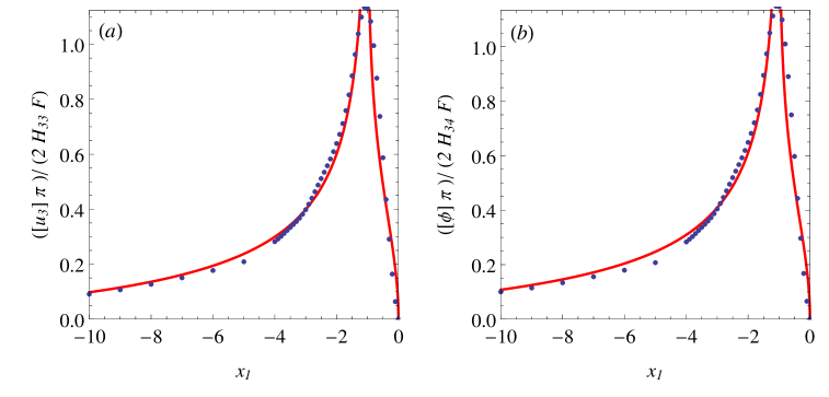
Figure 2: (a): Normalized displacement jump associate to symmetric mechanical loading localized in $x_{1}=a=-1$. Blue dots are COMSOL multiphysics results; (b): Normalized electric potential jump associate to symmetric mechanical loading localized in $x_{1}=a=1$. Blue dots are COMSOL multiphysics results.

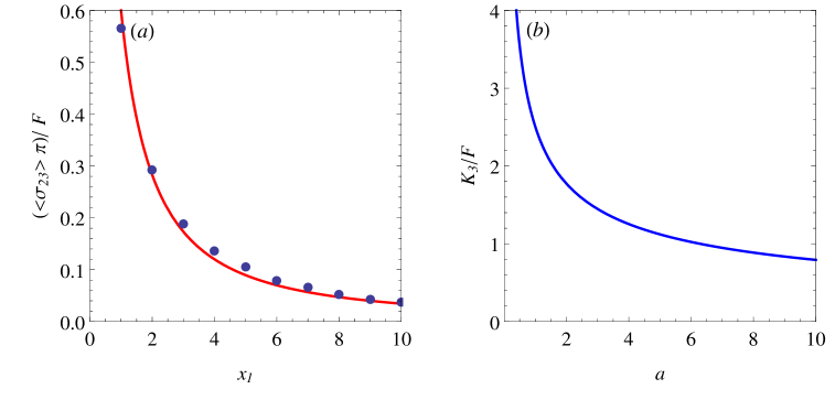
Figure 3: (a): Normalized shear traction associate to symmetric mechanical loading localized in $x_{1}=a=-1$. Blue dots are COMSOL multiphysics results; (b): Variation of the normalized stress intensity factor $K_{3}$ with the distance $a$ between te point of application of the load and the crack tip.

It is now possible to use (100) to obtain expressions for the stress intensity factor, $K_{3}$, and the electric intensity factor, $K_{4}$:

$$\begin{pmatrix}K_{3}\\ K_{4}\end{pmatrix}=\lim_{x_{1}\to 0}\sqrt{2\pi x_{1}}\begin{pmatrix}\sigma_{23}\\ D_{2}\end{pmatrix}=F\sqrt{\frac{2}{\pi a}}\begin{pmatrix}1\\ 0\end{pmatrix}.$$ (101)

Figures 2 and 3$/(b)$ show a comparison between the derived results and the equivalent results using finite element computations in COMSOL multiphysics. The point loads are assumed to be localized at a distance $a=-1$ from the crack tip, and the normalized crack opening, electric potential jump and shear traction profiles are reported as functions of the spatial coordinate $x_{1}$. The materials used above and below the crack were Barium Titanate and PZT respectively. The material parameters are quoted in Table 1, with those for Barium titanate obtained from Geis et al. [2] and those for PZT taken from Liu and Hsia [31].

Material	$C_{44}$(GPa)	$e_{15}$(CM2)	$\omega_{11}$(C2/Nm2
Barium Titanate	44	11.4	9.87 x 10-9
PZT	24.5	14.0	1.51 x 10-8

Table 1: Material properties

Good agreement between the analytical solution and the results provided by finite element analysis is detected in the figures for normalized crack opening, electric potential jump and shear traction field. The variation of the normalized stress intensity factor $K_{3}$ with the distance $a$ bewteen the crack tip and the point where the loads are applied is reported in Figure$/(b)$.

5.2.2 Asymmetric mechanical loading

The second example considered has point loadings at a distance $a$ acting on the upper and lower crack faces. However, for this asymmetric example it is said that they both act in the same direction (see for example Morini et al. [20]). Mathematically this is presented as:

$$\langle\mathbf{p}\rangle(x_{1})=0,\quad\llbracket\mathbf{p}\rrbracket(x_{1})=\begin{pmatrix}-2F\delta(x_{1}+a)\\ 0\end{pmatrix}.$$ (102)

It is important to note that, as just mentioned, most of the formulations previously proposed for fracture mechanics in piezoelectric bimaterials (see for example Suo et al. [3], Pak [30], Pan [6], Ma and Chen [15]), do not take into account the presence of skew-symmetric components of the load acting on the crack faces. Consequently, in order to solve crack problems involving non-symmetric loading distribution such as the (102), in Section 3 we have derived explicit expessions for the skew-symmetric weight functions matrices.

Taking into account the loading distribution (102), the singular integral equation (73) becomes

$$\mathbf{\mathcal{S}}^{(s)}\frac{\partial\llbracket\mathbf{u}\rrbracket^{(-)}}{\partial x_{1}}=-\frac{1}{2}\mathbf{W}\llbracket\mathbf{p}\rrbracket.$$ (103)

Using the same method as was used for the symmetric loading previously considered it is shown that

$$\begin{pmatrix}\llbracket u_{3}\rrbracket\\ \llbracket\phi\rrbracket\end{pmatrix}=\frac{2F}{\pi}\operatorname{arctanh}\sqrt{-\frac{x_{1}}{a}}\begin{pmatrix}\delta_{3}H_{33}\\ \gamma H_{34}\end{pmatrix},\quad\text{for }-a<x_{1}<0,$$ (104)

$$\begin{pmatrix}\llbracket u_{3}\rrbracket\\ \llbracket\phi\rrbracket\end{pmatrix}=\frac{2F}{\pi}\operatorname{arctanh}\sqrt{-\frac{a}{x_{1}}}\begin{pmatrix}\delta_{3}H_{33}\\ \gamma H_{34}\end{pmatrix},\quad\text{for }x_{1}<-a.$$ (105)

Making use of equation (74) it is possible to obtain the expression for the extended traction vector, $\mathbf{t}$, along the interface:

$$\mathbf{t}^{(+)}(x_{1}) =-\frac{\mathbf{H}^{-1}}{\pi}\int_{-\infty}^{0}\frac{1}{x_{1}-\eta}\frac{\partial\llbracket\mathbf{u}\rrbracket}{\partial\eta}\mathrm{d}\eta,$$

$$=\frac{F}{\pi}\sqrt{\frac{a}{x_{1}}}\frac{1}{x_{1}+a}\mathbf{H}^{-1}\begin{pmatrix}\delta_{3}H_{33}\\ \gamma H_{34}\end{pmatrix},$$

$$=\frac{F}{\pi}\sqrt{\frac{a}{x_{1}}}\frac{1}{x_{1}+a}\frac{1}{H_{33}H_{44}-H_{34}^{2}}\begin{pmatrix}\delta_{3}H_{33}H_{44}-\gamma H_{34}^{2}\\ (\gamma-\delta_{3})H_{33}H_{34}\end{pmatrix}.$$ (106)

It is now possible to use (106) to obtain expressions for the stress intensity factor, $K_{3}$, and the electric intensity factor, $K_{4}$:

$$\begin{pmatrix}K_{3}\\ K_{4}\end{pmatrix}=\lim_{x_{1}\to 0}\sqrt{2\pi x_{1}}\begin{pmatrix}t_{3}\\ D\end{pmatrix}=F\sqrt{\frac{2}{\pi a}}\frac{1}{H_{33}H_{44}-H_{34}^{2}}\begin{pmatrix}\delta_{3}H_{33}H_{44}-\gamma H_{34}^{2}\\ (\gamma-\delta_{3})H_{33}H_{34}\end{pmatrix}.$$ (107)

5.2.3 Symmetric electrical loading

We consider a symmetric system of electrical point loads on the crack faces at a distance $a$ behind the crack tip. Mathematically the Dirac delta distribution is once again to represent the forces:

$$\langle\mathbf{p}\rangle(x_{1})=\begin{pmatrix}0\\ -G\delta(x_{1}+a)\end{pmatrix},\quad\llbracket\mathbf{p}\rrbracket=\mathbf{0}.$$ (108)

Making use of equation (73) and the method previously used for mechanical loading gives

$$\frac{\partial\llbracket\mathbf{u}\rrbracket^{(-)}}{\partial x_{1}}=-\frac{G}{\pi}\sqrt{-\frac{a}{x_{1}}}\frac{1}{x_{1}+a}\begin{pmatrix}H_{34}\\ H_{44}\end{pmatrix}.$$ (109)

When integrated, this gives

$$\begin{pmatrix}\llbracket u_{3}\rrbracket\\ \llbracket\phi\rrbracket\end{pmatrix}=\frac{2G}{\pi}\operatorname{arctanh}\sqrt{-\frac{x_{1}}{a}}\begin{pmatrix}H_{34}\\ H_{44}\end{pmatrix},\quad\text{for }-a<x_{1}<0,$$ (110)

$$\begin{pmatrix}\llbracket u_{3}\rrbracket\\ \llbracket\phi\rrbracket\end{pmatrix}=\frac{2G}{\pi}\operatorname{arctanh}\sqrt{-\frac{a}{x_{1}}}\begin{pmatrix}H_{34}\\ H_{44}\end{pmatrix},\quad\text{for }x_{1}<-a.$$ (111)

The resulting expressions for the extended traction vector is therefore

$$\mathbf{t}^{(+)}(x_{1})=-\frac{\mathbf{H}^{-1}}{\pi}\int_{-\infty}^{0}\frac{1}{x_{1}-\eta}\frac{\partial\llbracket\mathbf{u}\rrbracket^{(-)}}{\partial\eta}\mathrm{d}\eta=\frac{G}{\pi}\sqrt{\frac{a}{x_{1}}}\frac{1}{x_{1}+a}\begin{pmatrix}0\\ 1\end{pmatrix}.$$ (112)

The stress intensity factors are then given by

$$\begin{pmatrix}K_{3}\\ K_{4}\end{pmatrix}=\lim_{x_{1}\to 0}\sqrt{2\pi x_{1}}\mathbf{t}^{(+)}(x_{1})=G\sqrt{\frac{2}{\pi a}}\begin{pmatrix}0\\ 1\end{pmatrix}.$$ (113)

5.2.4 Asymmetric electrical loading

Here we consider electrical loading acting in the same direction on the top and bottom crack faces at a distance $a$ behind the crack tip. This loading can be written as

$$\langle\mathbf{p}\rangle(x_{1})-\mathbf{0},\quad\llbracket\mathbf{p}\rrbracket(x_{1})=\begin{pmatrix}0\\ -2G\delta(x_{1}+a)\end{pmatrix}.$$ (114)

Similarly to the case of asymmetric mechanical load (102), in order to derive the crack opening and the traction fields ahead of the tip corresponding to the asymmetric electrical loading distribution (114), the approaches proposed by Suo et al. [3], Pak [30], Pan [6], Ma and Chen [15] need to be generalized to the case of non-symmetric electrical loading applied to the crack faces. As a consequence, the skew-symmetric weight function matrices derived in Section 3 are required. Assuming that the loading function is given by expression (114), the resulting fields obtained using equations (73) and (74) are:

$$\frac{\partial\llbracket\mathbf{u}\rrbracket^{(-)}}{\partial x_{1}}=-\frac{G}{\pi}\sqrt{-\frac{a}{x_{1}}}\frac{1}{x_{1}+a}\begin{pmatrix}\gamma H_{34}\\ \delta_{4}H_{44}\end{pmatrix},$$ (115)

$$\begin{pmatrix}\llbracket u_{3}\rrbracket\\ \llbracket\phi\rrbracket\end{pmatrix}=\frac{2G}{\pi}\operatorname{arctanh}\sqrt{-\frac{x_{1}}{a}}\begin{pmatrix}\gamma H_{34}\\ \delta_{4}H_{44}\end{pmatrix},\quad\text{for }-a<x_{1}<0,$$ (116)

$$\begin{pmatrix}\llbracket u_{3}\rrbracket\\ \llbracket\phi\rrbracket\end{pmatrix}=\frac{2G}{\pi}\operatorname{arctanh}\sqrt{-\frac{a}{x_{1}}}\begin{pmatrix}\gamma H_{34}\\ \delta_{4}H_{44}\end{pmatrix},\quad\text{for }x_{1}<-a.$$ (117)

$$\mathbf{t}^{(+)}(x_{1})=\frac{G}{\pi}\sqrt{\frac{a}{x_{1}}}\frac{1}{(x_{1}+a)(H_{33}H_{44}-H_{34}^{2})}\begin{pmatrix}(\gamma-\delta_{4})H_{34}H_{44}\\ \delta_{4}H_{33}H_{44}-\gamma H_{34}^{2}\end{pmatrix}.$$ (118)

The stress intensity factor and electric intensity factor obtained are therefore

$$\begin{pmatrix}K_{3}\\ K_{4}\end{pmatrix}=\lim_{x_{1}\to 0}\sqrt{2\pi x_{1}}\mathbf{t}^{(+)}(x_{1})=G\sqrt{\frac{2}{\pi a}}\frac{1}{H_{33}H_{44}-H_{34}^{2}}\begin{pmatrix}(\gamma-\delta_{4})H_{34}H_{44}\\ \delta_{4}H_{33}H_{44}-\gamma H_{34}^{2}\end{pmatrix}.$$ (119)

6 Conclusions

A general approach for the derivation of the symmetric and skew-symmetric weight functions for plane interfacial cracks in anisotropic piezoelectric bimaterials have been developed. The method proposed by Morini et al. [17] and Pryce et al. [18] for anisotropic elastic bodies, based on the Stroh formalism and Riemann-Hilbert formulation, has been extended for studying crack problems at the interface between dissimilar piezoelectric media. Applying this approach, explicit weight function matrices are obtained for an interfacial crack between two transversely isotropic piezoelectric materials, considering both the case where the poling direction of the two materials is perpendicular and coincident to the crack front. Since many poled ceramics that are commonly used in industrial applications possess transversely isotropic symmetry, this class of piezoelectric materials has a practical significance, and the derived weight functions can be used for computing the stress intensity factors corresponding to any arbitrary non-symmetric mechanical and electrostatic load acting on the crack faces [8].

Symmetric and skew-symmetric weight function matrices are used together with Betti’s reciprocity theorem to derive integral identities relating the applied loading functions to the corresponding crack opening and tractions ahead of the tip. By means of the proposed method, an explicit singular integral formulation for the crack problem is obtained avoiding the use of Green’s function and the challenging numerical calculations related to such an approach. Integral identities have been derived for interfacial crack problems between dissimilar transversely isotropic piezoceramics subject to the two-dimensional state of plane strain and short circuit, having poling direction perpendicular or coincident to the crack front. An example of the application of the integral identities to crack problems where the loading is given by punctual forces acting on the faces has been performed. Explicit expressions for crack opening and tractions ahead of the tip corresponding to both symmetric and skew-symmetric mechanical and electrical loading have been obtained. The stress intensity factors associated with the introduced loading configurations are also evaluated. Using the derived skew-symmetric weight functions matrices, in the illustrative examples the effects of asymmetric loading configurations, which cannot be considered applying the alternative formulations available in literature, are studied. For the case where the poling direction is perpendicular to the $x_{3}-$axis and symmetric loading is applied at the faces, the results obtained by the solution of the singular integral equations are compared with those performed by finite element analysis using COMSOL Multiphysics. Good agreement between the analytical expression for the crack opening obtained by the singular integral identities and the numerical results is detected.

Thanks to the versatility of the Stroh formalism and the generality of Betti’s theorem, the developed approach can be easily adapted for studying several fracture problems in piezoelectric materials with many different properties without any assumption concerning the symmetry of the applied loads. Furthermore, the derived integral identities also have their own value from the mathematical point of view, as, to the authors best knowledge, such identities written in a similar explicit form for interfacial cracks in anisotropic piezoelectric bimaterials seem to be unknown in the literature.

Appendix A Derivation of the Betti formula for piezoelectric materials

In this Appendix the derivation of the generalized Betti identity for piezoelectric materials is reported. Two sets of stresses, strains, electric fields and electrical displacements acting on the same physical space are assumed. The two sets of fields are denoted by the superscripts ⁽¹⁾ and ⁽²⁾, respectively. The equations relating these fields are [24]:

$$\sigma_{ij}^{(1)}\varepsilon_{ij}^{(2)}-D_{j}^{(1)}E_{j}^{(2)}=\sigma_{ij}^{(2)}\varepsilon_{ij}^{(1)}-D_{j}^{(2)}E_{j}^{(1)}.$$ (120)

Taking the integral of (120) over a volume, $V$, in combination with equation (3) yields

$$\int_{V}\left[(\sigma_{ij}^{(1)}u_{i}^{(2)})_{,j}+(D_{j}^{(1)}\phi^{(2)})_{,j}\right]\mathrm{d}V=\int_{V}\left[(\sigma_{ij}^{(2)}u_{i}^{(1)})_{,j}+(D_{j}^{(2)}\phi^{(1)})_{,j}\right]\mathrm{d}V.$$ (121)

Making use of the Divergence Theorem and then rearranging gives

$$\int_{S}\left[\sigma_{ji}^{(1)}n_{j}u_{i}^{(2)}+D_{j}^{(1)}n_{j}\phi^{(2)}-\sigma_{ji}^{(2)}n_{j}u_{i}^{(1)}-D_{j}^{(2)}n_{j}\phi^{(1)}\right]\mathrm{d}S=0,$$ (122)

where $S$ is the boundary of the volume $V$.

Taking $V$ to be a hemisphere in the upper half-plane with flat edge along the $x_{2}-$plane in equation (122) leads to the following equation:

$$\int_{x_{2}=0^{+}}\left[\sigma_{2i}^{(1)}u_{i}^{(2)}+D_{2}^{(1)}\phi^{(2)}-\sigma_{2i}^{(2)}u_{i}^{(1)}-D_{2}^{(2)}\phi^{(1)}\right]\mathrm{d}x_{1}=0,$$ (123)

which can written in terms of the extended displacement and traction vectors used in this paper

$$\int_{x_{2}=0^{+}}\left[\mathbf{t}^{(1)}\cdot\mathbf{u}^{(2)}-\mathbf{t}^{(2)}\cdot\mathbf{u}^{(1)}\right]\mathrm{d}x_{1}.$$ (124)

To obtain equation (26) $\mathbf{u}^{(1)}$ and $\mathbf{t}^{(1)}$ are taken as the physical fields and then $\mathbf{u}^{(2)}=\mathbf{R}\mathbf{U}$ and $\mathbf{t}^{(2)}=\mathbf{R}\mathbf{\Sigma}$. Equation (27) is derived using a semi-circular domain in the lower half-plane.

Appendix B Transversely isotropic piezoelectric materials: explicit expressions for matrices $\mathbf{Q}$, $\mathbf{R}$ and $\mathbf{T}$

In this Appendix, explicit expressions for the stiffness, permittivity and piezoelectric tensors corresponding to transversely isotropic piezoelectric materials with poling direction parallel to the $x_{2}$ and $x_{3}$ axes are reported. Using these tensors, general forms for the Stroh’s eigenvalues matrices, the surface admittance tensor and the bimaterial matrices $\mathbf{H}$ and $\mathbf{W}$ are obtained.

B.1 Poling direction parallel to the $x_{2}-$axis

When considering transverse isotropic materials with poling direction parallel to the $x_{2}$-axis the stiffness tensor, $\mathbf{C}$, simplifies to

$$\mathbf{C}=\begin{pmatrix}C_{11}&C_{12}&C_{13}&0&0&0\\ C_{12}&C_{22}&C_{12}&0&0&0\\ C_{13}&C_{12}&C_{11}&0&0&0\\ 0&0&0&C_{44}&0&0\\ 0&0&0&0&(C_{11}-C_{13})/2&0\\ 0&0&0&0&0&C_{44}\end{pmatrix},$$

and the permittivity and piezoelectric tensors simplify to

$$\mathbf{\omega}=\begin{pmatrix}\omega_{11}&0&0\\ 0&\omega_{22}&0\\ 0&0&\omega_{11}\end{pmatrix},\qquad\mathbf{e}=\begin{pmatrix}0&0&0&0&0&e_{16}\\ e_{21}&e_{22}&e_{21}&0&0&0\\ 0&0&0&e_{16}&0&0\end{pmatrix}.$$

This is the same system as used in Hwu [22]. Using these conditions the matrices from equation (6) reduce to

$$\mathbf{Q}=\begin{pmatrix}C_{11}&0&0&0\\ 0&C_{44}&0&e_{16}\\ 0&0&(C_{11}-C_{13})/2&0\\ 0&e_{16}&0&-\omega_{11}\end{pmatrix},\quad\mathbf{R}=\begin{pmatrix}0&C_{12}&0&e_{21}\\ C_{44}&0&0&0\\ 0&0&0&0\\ e_{16}&0&0&0\end{pmatrix},$$

$$\mathbf{T}=\begin{pmatrix}C_{44}&0&0&0\\ 0&C_{22}&0&e_{22}\\ 0&0&C_{44}&0\\ 0&e_{22}&0&-\omega_{22}\end{pmatrix}.$$

Note that in this case the poling direction is perpendicular to the crack plane reported in Fig. 1. The antiplane component can clearly be decoupled from the rest of the elasticity components and all effects caused by the electric field. This means that the Mode III tractions and displacement have no dependency on the electric field and therefore behave in the same way as they would in an elastic material with no piezoelectric effect.

Only the in-plane components and electrical effects are considered. That is: $\mathbf{u}=(u_{1},u_{2},\phi)^{T}$ and $\mathbf{t}=(\sigma_{21},\sigma_{22},D_{2})^{T}$. The decoupled part of the eigenvalue problem (6) now has matrices

$$\mathbf{Q}=\begin{pmatrix}C_{11}&0&0\\ 0&C_{44}&e_{16}\\ 0&e_{16}&-\omega_{11}\end{pmatrix},\quad\mathbf{R}=\begin{pmatrix}0&C_{12}&e_{16}\\ C_{44}&0&0\\ e_{21}&0&0\end{pmatrix},$$

$$\mathbf{T}=\begin{pmatrix}C_{44}&0&0\\ 0&C_{11}&e_{22}\\ 0&e_{22}&-\omega_{22}\end{pmatrix}.$$ (125)

The extended Stroh formalism described in Section 2 of the paper is an effective tool for finding an expression for the surface admittance tensor, $\mathbf{B}$. However, the eigenvalue problem obtained is not always straightforward to solve. For non-piezoelectric materials an alternative approach is the Lekhnitskii formalism introduced by Lekhnitskii [32] which gives a specific normalisation of the eigenvalues obtained from the eigenvalue problem (6) [33]. The Lekhnitskii formalism was extended to the piezoelectric setting by Hwu [22] where it was used to find the surface admittance tensor for the poling direction parallel to the $x_{2}$-axis

$$\mathbf{B}=\begin{pmatrix}B_{11}&iB_{12}&iB_{14}\\ -iB_{12}&B_{22}&B_{24}\\ -iB_{14}&B_{24}&B_{44}\end{pmatrix}.$$ (126)

The expressions for the components of the matrix $\mathbf{B}$ found by Hwu [22] are quoted in the Appendix C.

With an expression for $\mathbf{B}$ it is now possible to construct the bimaterial matrices required. The bimaterial matrix $\mathbf{H}$ can be written as

$$\mathbf{H}=\begin{pmatrix}H_{11}&iH_{12}&iH_{14}\\ -iH_{12}&H_{22}&H_{24}\\ -iH_{14}&H_{24}&H_{44}\end{pmatrix},$$ (127)

where

$$H_{\alpha\alpha}=[B_{\alpha\alpha}]_{I}+[B_{\alpha\alpha}]_{II},\quad\text{for }\alpha=1,2,4,$$

$$H_{1\beta}=[B_{1\beta}]_{I}-[B_{1\beta}]_{II},\quad\text{for }\beta=2,4,$$

$$H_{24}=[B_{24}]_{I}+[B_{24}]_{II}.$$

The matrix $\mathbf{W}$ has the same structure as $\mathbf{H}$, that is

$$\mathbf{W}=\begin{pmatrix}W_{11}&iW_{12}&iW_{14}\\ -iW_{12}&W_{22}&W_{24}\\ -iW_{14}&W_{24}&W_{44}\end{pmatrix},$$ (128)

where

$$W_{\alpha\alpha}=[B_{\alpha\alpha}]_{I}-[B_{\alpha\alpha}]_{II},\quad\text{for }\alpha=1,2,4,$$

$$W_{1\beta}=[B_{1\beta}]_{I}+[B_{1\beta}]_{II},\quad\text{for }\beta=2,4,$$

$$W_{24}=[B_{24}]_{I}-[B_{24}]_{II}.$$

B.2 Poling direction parallel to the $x_{3}-$axis

When considering transverse isotropic materials with poling direction parallel to the $x_{3}$-axis the stiffness tensor, $C$, simplifies to

$$C=\begin{pmatrix}C_{11}&C_{12}&C_{13}&0&0&0\\ C_{12}&C_{11}&C_{13}&0&0&0\\ C_{13}&C_{13}&C_{33}&0&0&0\\ 0&0&0&C_{44}&0&0\\ 0&0&0&0&C_{44}&0\\ 0&0&0&0&0&(C_{11}-C_{12})/2\end{pmatrix},$$

and the permittivity and piezoelectric tensors simplify to

$$\omega=\begin{pmatrix}\omega_{11}&0&0\\ 0&\omega_{11}&0\\ 0&0&\omega_{33}\end{pmatrix},\qquad e=\begin{pmatrix}0&0&0&0&e_{15}&0\\ 0&0&0&e_{15}&0&0\\ e_{31}&e_{31}&e_{33}&0&0&0\end{pmatrix}.$$

Using these conditions the matrices from equation (6) reduce to

$$\mathbf{Q}=\begin{pmatrix}C_{11}&0&0&0\\ 0&(C_{11}-C_{12})/2&0&0\\ 0&0&C_{44}&e_{15}\\ 0&0&e_{15}&-\omega_{11}\end{pmatrix},\quad\mathbf{R}=\begin{pmatrix}0&C_{12}&0&0\\ (C_{11}-C_{12})/2&0&0&0\\ 0&0&0&0\\ 0&0&0&0\end{pmatrix},$$

$$\mathbf{T}=\begin{pmatrix}(C_{11}-C_{12})/2&0&0&0\\ 0&C_{11}&0&0\\ 0&0&C_{44}&e_{15}\\ 0&0&e_{15}&-\omega_{11}\end{pmatrix}.$$

Note that in this case the poling direction coincides with the front of the crack reported in Fig. 1. For this particular case it is possible to decouple the Mode I and Mode II components of the displacement and stress fields from the Mode III fields and piezoelectric effects on the material. This means that the Mode I and II fields will behave similarly to those for purely elastic materials with no piezoelectric behaviour.

Only the out-of-plane and piezoelectric components are considered. In this case $\mathbf{Q}$, $\mathbf{R}$ and $\mathbf{T}$ are reduced to 2x2 matrices:

$$\mathbf{Q}=\mathbf{T}=\begin{pmatrix}C_{44}&e_{15}\\ e_{15}&-\omega_{11}\end{pmatrix},\qquad\mathbf{R}=\mathbf{0}.$$ (129)

As a consequence, for this case the surface admittance tensor, $\mathbf{B}$ assumes the form

$$\mathbf{B}=\begin{pmatrix}B_{33}&B_{34}\\ B_{34}&B_{44}\end{pmatrix}.$$ (130)

Explicit expressions for the components of $\mathbf{B}$ are given in the Appendix C.

The bimaterial matrices $\mathbf{H}$ and $\mathbf{W}$ can be computed and have the form

$$\mathbf{H}=\begin{pmatrix}H_{33}&H_{34}\\ H_{34}&H_{44}\end{pmatrix},\qquad\mathbf{W}=\begin{pmatrix}\delta_{3}H_{33}&\gamma H_{34}\\ \gamma H_{34}&\delta_{4}H_{44}\end{pmatrix}.$$ (131)

The components of these matrices are given by

$$H_{\alpha\beta}=[B_{\alpha\beta}]_{I}+[B_{\alpha\beta}]_{II},\quad\text{for }\alpha,\beta=3,4,$$

$$\delta_{\alpha}=\frac{[B_{\alpha\alpha}]_{I}-[B_{\alpha\alpha}]_{II}}{[B_{\alpha\alpha}]_{I}+[B_{\alpha\alpha}]_{II}},\quad\text{for }\alpha=3,4,$$

$$\gamma=\frac{[B_{34}]_{I}-[B_{34}]_{II}}{H_{34}}.$$

Appendix C Explicit expressions for $\mathbf{B}=i\mathbf{AL}^{-1}$

In this section we give the expressions for the surface admittance tensor $\mathbf{B}$ corresponding to the two-dimensional state of plane strain and short circuit ($\varepsilon_{3}=0,E_{3}=0$), as seen in Hwu [22]. We only give the expressions for the decoupled part of the tensor which contains the piezoelectric behaviour of the material.

C.1 Poling direction parallel to the $x_{2}$-axis

As stated in Section 2, the general form of the matrix $\mathbf{B}=i\mathbf{AL}^{-1}$ for transverse isotropic materials with poling direction parallel to the $x_{2}$-axis is

$$\mathbf{B}=\begin{pmatrix}B_{11}&iB_{12}&iB_{14}\\ -iB_{12}&B_{22}&B_{24}\\ -iB_{14}&B_{24}&B_{44}\end{pmatrix}.$$ (132)

Here, explicit expressions for the components of this matrix (found in Hwu [22]) are given.

The following components of the compliance tensor: $\mathbf{S}$, piezoelectric strain/voltage tensor: $\mathbf{g}$, and dielectric non-permittivity: $\mathbf{\beta}$, are introduced:

$$\hat{S^{\prime}}_{11} =\frac{C_{22}}{C_{11}C_{22}-C_{12}^{2}}-\frac{(e_{21}C_{11}-e_{22}C_{12})^{2}}{C^{*}[C_{11}C_{22}-C_{12}^{2}]},$$

$$\hat{S^{\prime}}_{12} =-\frac{e_{21}e_{22}[C_{11}^{2}-C_{12}^{2}]}{C^{*}[C_{11}C_{22}-C_{12}^{2}]}+\frac{\omega_{22}C_{12}}{C^{*}},$$

$$\hat{S^{\prime}}_{22} =\frac{e_{21}^{2}[C_{11}^{2}-C_{12}^{2}]}{C^{*}[C_{11}C_{22}-C_{12}^{2}]}+\frac{\omega_{22}C_{11}}{C^{*}},$$

$$\hat{S^{\prime}}_{66} =\frac{\omega_{11}}{e_{16}^{2}+\omega_{11}C_{44}},$$

$$\hat{g^{\prime}}_{21} =\frac{e_{21}C_{11}-e_{22}C_{12}}{C^{*}},$$

$$\hat{g^{\prime}}_{22} =\frac{e_{22}C_{11}-e_{21}C_{12}}{C^{*}},$$

$$\hat{g^{\prime}}_{16} =\frac{e_{16}}{e_{16}^{2}+\omega_{11}C_{44}},$$

$$\hat{\beta^{\prime}}_{11} =\frac{C_{44}}{e_{16}^{2}+\omega_{11}C_{44}},$$

$$\hat{\beta^{\prime}}_{22} =\frac{C_{11}C_{22}-C_{12}^{2}}{C^{*}},$$

where

$$C^{*}=(e_{21}^{2}+e_{22}^{2})C_{11}-2e_{21}e_{22}C_{12}+\omega_{22}[C_{11}C_{22}-C_{12}^{2}].$$

Through using the Lekhnitskii formalism extended to piezoelectric materials the eigenvalues, $p$, are found through the equation

$$l_{4}\rho_{2}-m_{3}^{2}=0,$$ (133)

where $l_{4},\rho_{2}$ and $m_{3}$ are functions of $p$ and are given by

$$l_{4}=\hat{S^{\prime}}_{11}p^{4}+(2\hat{S^{\prime}}_{12}+\hat{S^{\prime}}_{66})p^{2}+\hat{S^{\prime}}_{22},\quad m_{3}=-(\hat{g^{\prime}}_{21}+\hat{g^{\prime}}_{16})p^{2}-\hat{g^{\prime}}_{22},\quad\rho_{2}=-(\hat{\beta^{\prime}}_{11}p^{2}+\hat{\beta^{\prime}}_{22}).$$ (134)

This sextic equation must be solved numerically but is easily shown to have roots of the form

$$p_{2}=\alpha_{2}+i\beta_{2},\quad p_{3}=-\alpha_{2}+i\beta_{2},\quad p_{4}=i\beta_{4}.$$ (135)

With the eigenvalues known, Hwu [22] proceeded to find explicit expressions for the components of $\mathbf{B}$. It was shown that

$$B_{11} =2\hat{S^{\prime}}_{11}\mathrm{Im}\{p_{2}^{2}\bar{\eta_{2}}+(p_{4}^{2}\eta_{2}-p_{2}^{2}\eta_{4})\}/\lambda,$$

$$B_{22} =2\mathrm{Im}\{[\gamma_{2}\bar{p_{2}}p_{4}\eta_{4}+(\gamma_{2}p_{4}^{2}-\gamma_{4}p_{2}^{2})\bar{\eta_{2}}]/p_{2}p_{4}\}/\lambda,$$

$$B_{44} =-2\hat{\beta^{\prime}}_{11}\mathrm{Im}\{p_{2}\bar{p_{2}}\eta_{2}+p_{2}p_{4}(\eta_{2}-\eta_{4})\}/\lambda,$$

$$B_{24} =2\hat{\beta^{\prime}}_{11}\mathrm{Im}\{p_{2}\bar{p_{2}}\eta_{2}\eta_{4}+p_{2}p_{4}\bar{\eta_{2}}(\eta_{2}-\eta_{4})\}/\lambda,$$

$$B_{12} =\hat{S^{\prime}}_{12}+2\mathrm{Re}\{[\gamma_{2}p_{4}\eta_{2}+(\gamma_{4}p_{2}\eta_{2}-\gamma_{2}p_{4}\eta_{4})]/p_{2}p_{4}\}/\lambda,$$

$$B_{14} =-\hat{g^{\prime}}_{16}+2\hat{\beta^{\prime}}_{11}\mathrm{Re}\{p_{2}\eta_{2}\bar{\eta_{2}}-\eta_{2}\eta_{4}(p_{2}-p_{4})\}/\lambda,$$

where

$$\lambda=2\mathrm{Re}\{\bar{p_{2}}\eta_{2}+(p_{4}\eta_{2}-p_{2}\eta_{4})\},$$

$$\gamma_{k}=\hat{S^{\prime}}_{22}+\hat{g^{\prime}}_{22}\eta_{k},\quad\eta_{k}=\frac{l_{4}(p_{k})}{m_{3}(p_{k})},\quad\text{for k=2,4}.$$

C.2 Poling direction parallel to the $x_{3}$-axis

The decoupled part of the surface admittance tensor, $\mathbf{B}=i\mathbf{AL}^{-1}$, containing Mode III fields and the piezoelectric effect for transverse isotropic materials with poling direction parallel to the $x_{3}$-axis is:

$$\mathbf{B}=\begin{pmatrix}B_{33}&B_{34}\\ B_{34}&B_{44}\end{pmatrix}.$$ (136)

Explicit expressions for the components of this matrix are given by:

$$B_{33}=\frac{\omega_{11}}{e_{15}^{2}+\omega_{11}C_{44}},$$

$$B_{44}=\frac{-C_{44}}{e_{15}^{2}+\omega_{11}C_{44}},$$

$$B_{34}=\frac{e_{15}}{e_{15}^{2}+\omega_{11}C_{44}}.$$

Appendix D Inverse Fourier transforms

In order to derive explicit expressions for equations (60) and (61), we need to compute the inverse Fourier trasform of terms of the form $i\mathrm{sign}(\xi)\hat{f}(\xi)$, $|\xi|\hat{f}(\xi)$ and $i\xi\hat{f}(\xi)$. Using the Fourier convolution theorem and the knowledge that the inverse Fourier transform of $\mathrm{sign}(\xi)$ is given by $-i/(\pi x_{1})$ gives:

$$\mathcal{F}^{-1}[i\mathrm{sign}(\xi)\hat{f}(\xi)] =i\mathcal{F}^{-1}[\mathrm{sign}(\xi)]\ast\mathcal{F}^{-1}[\hat{f}(\xi)],$$

$$=i\Big{(}\frac{-i}{\pi x_{1}}\Big{)}\ast f(x_{1}),$$

$$=\frac{1}{\pi}\int^{\infty}_{-\infty}\frac{f(\eta)}{x_{1}-\eta}\mathrm{d}\eta.$$ (137)

The inverse Fourier transform of $|\xi|\hat{f}(\xi)$ is found:

$$\mathcal{F}^{-1}[|\xi|\hat{f}(\xi)] =\mathcal{F}^{-1}[\mathrm{sign}(\xi)]\ast\mathcal{F}^{-1}[\xi\hat{f}(\xi)],$$

$$=\Big{(}-\frac{i}{\pi x_{1}}\Big{)}\ast i\frac{\partial f}{\partial x_{1}},$$

$$=\Big{(}\frac{1}{\pi x_{1}}\Big{)}\ast\frac{\partial f}{\partial x_{1}}.$$ (138)

Finally, the inverse Fourier transform of $i\mathrm{sign}(\xi)|\xi|\hat{f}(\xi)$ is given by

$$\mathcal{F}^{-1}[i\mathrm{sign}(\xi)|\xi|\hat{f}(\xi)] =\mathcal{F}^{-1}[i\xi\hat{f}(\xi)],$$

$$=-\frac{\partial f}{\partial x_{1}}.$$ (139)

Appendix E Expressions for matrices $\mathbf{M}$ and $\mathbf{N}$

In this Appendix explicit expressions for the matrices $\mathbf{M}$ and $\mathbf{N}$ are quoted. They have the form

$$\mathbf{M}=\frac{1}{2D}\left(\mathbf{M}^{\prime}+i\mathrm{sign}(\xi)\mathbf{M}^{\prime\prime}\right),$$ (140)

$$\mathbf{N}=\frac{|\xi|}{D}\left(\mathbf{N}^{\prime}+i\mathrm{sign}(\xi)\mathbf{N}^{\prime\prime}\right),$$ (141)

where

$$D=H_{14}^{2}H_{22}+H_{12}^{2}H_{44}+H_{24}^{2}H_{11}-H_{11}H_{22}H_{44}-2H_{14}H_{12}H_{24}.$$ (142)

The matrices $\mathbf{M}^{\prime},\mathbf{M}^{\prime\prime},\mathbf{N}^{\prime}$ and $\mathbf{N}^{\prime\prime}$ have the form

$$\mathbf{M}^{\prime}=\begin{pmatrix}M_{11}&0&0\\ 0&M_{22}&M_{24}\\ 0&M_{42}&M_{44}\end{pmatrix},\qquad\mathbf{M}^{\prime\prime}=\begin{pmatrix}0&M_{12}&M_{14}\\ M_{21}&0&0\\ M_{41}&0&0\end{pmatrix},$$ (143)

$$\mathbf{N}^{\prime}=\begin{pmatrix}N_{11}&0&0\\ 0&N_{22}&N_{24}\\ 0&N_{24}&N_{44}\end{pmatrix},\qquad\mathbf{N}^{\prime\prime}=\begin{pmatrix}0&N_{12}&N_{14}\\ -N_{12}&0&0\\ -N_{14}&0&0\end{pmatrix},$$ (144)

where

$$M_{11} =W_{11}(H_{24}^{2}-H_{22}H_{44})+W_{12}(H_{12}H_{44}-H_{14}H_{24})-W_{14}(H_{12}H_{24}-H_{14}H_{22}),$$ (145)

$$M_{22} =W_{12}(H_{12}H_{44}-H_{14}H_{24})-W_{22}(H_{11}H_{44}-H_{14}^{2})-W_{24}(H_{14}H_{12}-H_{11}H_{24}),$$ (146)

$$M_{44} =W_{14}(H_{14}H_{22}-H_{12}H_{24})-W_{24}(H_{14}H_{12}-H_{11}H_{24})-W_{44}(H_{11}H_{22}-H_{12}^{2}),$$ (147)

$$M_{24} =W_{14}(H_{14}H_{24}-H_{12}H_{44})+W_{24}(H_{11}H_{44}-H_{14}^{2})+W_{44}(H_{14}H_{12}-H_{11}H_{24}),$$ (148)

$$M_{42} =W_{12}(H_{12}H_{24}-H_{14}H_{22})+W_{22}(H_{14}H_{12}-H_{11}H_{24})+W_{24}(H_{11}H_{22}-H_{12}^{2}),$$ (149)

$$M_{12} =W_{12}(H_{22}H_{44}-H_{24}^{2})-W_{22}(H_{12}H_{44}-H_{14}H_{24})+W_{24}(H_{12}H_{24}-H_{14}H_{22}),$$ (150)

$$M_{14} =W_{14}(H_{24}^{2}-H_{22}H_{44})+W_{24}(H_{12}H_{44}-H_{14}H_{24})-W_{44}(H_{12}H_{24}-H_{14}H_{22}),$$ (151)

$$M_{21} =W_{11}(H_{12}H_{44}-H_{14}H_{24})-W_{12}(H_{11}H_{44}-H_{14}^{2})-W_{14}(H_{14}H_{12}-H_{11}H_{24}),$$ (152)

$$M_{41} =W_{11}(H_{12}H_{24}-H_{14}H_{22})+W_{12}(H_{14}H_{12}-H_{11}H_{24})+W_{14}(H_{11}H_{22}-H_{12}^{2}),$$ (153)

$$N_{11} =H_{22}H_{44}-H_{24}^{2},$$ (154)

$$N_{22} =H_{11}H_{44}-H_{14}^{2},$$ (155)

$$N_{44} =H_{11}H_{22}-H_{12}^{2},$$ (156)

$$N_{24} =H_{11}H_{24}-H_{14}H_{12},$$ (157)

$$N_{12} =H_{12}H_{44}-H_{14}H_{24},$$ (158)

$$N_{14} =H_{12}H_{24}-H_{14}H_{22}.$$ (159)

Appendix F Expressions for matrices $\mathbf{Y}$ and $\mathbf{Z}(\xi)$

Explicit expressions for the matrices $\mathbf{Y}$ and $\mathbf{Z}(\xi)$ are given by:

$$\mathbf{Y}=\frac{1}{2}\mathbf{H}^{-1}\mathbf{W}=\frac{1}{2(H_{33}H_{44}-H_{34}^{2})}\begin{pmatrix}\delta_{3}H_{33}H_{44}-\gamma H_{34}^{2}&H_{44}H_{34}(\gamma-\delta_{4})\\ H_{33}H_{34}(\gamma-\delta_{3})&\delta_{4}H_{33}H_{44}-\gamma H_{34}^{2}\end{pmatrix},$$ (160)

$$\mathbf{Z}(\xi)=-\frac{|\xi|}{H_{33}H_{44}-H_{34}^{2}}\begin{pmatrix}H_{44}&-H_{34}\\ -H_{34}&H_{33}\end{pmatrix}.$$ (161)

References

- Barnett and Lothe [1975] D. M. Barnett and J. Lothe. Dislocations and line charges in anisotropic piezoelectric insulators. Phys. Stat. Sol. B, 67:105–111, 1975.
- Geis et al. [2004] W. Geis, G. Mishuris, and A. Sandig. Asymptotic models for piezoelectric stack actuators with thin metal inclusions. Preprint 2004/001, Univeristy of Stuttgart, http://preprints.ians.uni-stuttgart.de, 2004.
- Suo et al. [1992] Z. Suo, C. M. Kuo, D. M. Barnett, and J. R. Willis. Fracture mechanics for piezoelectric ceramics. J. Mech. Phys. Solids, 40:739–765, 1992.
- Stroh [1962] A. N. Stroh. Steady state problems in anisotropic elasticity. Math. Phys, 41:77–103, 1962.
- Gao and Wang [2001] C.-F. Gao and M.-Z. Wang. Green’s functions for an interfacial crack between two dissimilar piezoelectric media. Int. J. Solids Struct., 38:5323–5334, 2001.
- Pan [2003] E. Pan. Some new three-dimensional green’s functions in anisotropic piezoelectric bimaterials. Electron. J. Bound. Elem., 1:236–269, 2003.
- Pan and Yuan [2000] E. Pan and F. G. Yuan. Three-dimensional green’s functions in anisotropic piezoelectric bimaterials. Int. J. Eng. Sci., 38:1939–1960, 2000.
- Piccolroaz et al. [2009] A. Piccolroaz, G. Mishuris, and A. B. Movchan. Symmetric and skew-symmetric weight functions in 2d perturbation models for semi-infinite interfacial cracks. J. Mech. Phys. Solids, 57:1657–1682, 2009.
- Piccolroaz and Mishuris [2013] A. Piccolroaz and G. Mishuris. Integral identities for a semi-infinite interfacial crack in 2d and 3d elasticity. J. Elasticity, 110:117–140, 2013.
- Bueckner [1970] H. F. Bueckner. A novel principle for the computation of stress intensity factors. Zeit. Ang. Math. Mech., 50:529–546, 1970.
- Bueckner [1985] H. F. Bueckner. Weight functions and fundamental fields for the penny-shaped and the half plane crack in three-space. Int. J. Solids Struct., 23:57–93, 1985.
- Bueckner [1989] H. F. Bueckner. Observations on weight functions. Eng. Anal. Bound. Elem., 6:3–18, 1989.
- Rice [1972] J. R. Rice. Some remarks on elastic crack-tip stress fields. Int. J. Solids Struct., 8:751–758, 1972.
- McMeeking and Ricoeur [2003] R. McMeeking and A. Ricoeur. The weight functions for crack in piezoelectrics. Int. J. Solids Struct., 40:6143–6162, 2003.
- Ma and Chen [2001] L.-F. Ma and Y.-H. Chen. Weight functions for interface cracks in dissimilar anisotropic piezoelectric materials. Int. J. Fract., 110:263–279, 2001.
- Willis and Movchan [1995] J. R. Willis and A. B. Movchan. Dynamic weight function for a moving crack. i. mode i loading. J. Mech. Phys. Solids, pages 319–341, 1995.
- Morini et al. [2013a] L. Morini, E. Radi, A. B. Movchan, and N. V. Movchan. Stroh formalism in analysis of skew-symmetric and symmetric weight functions for interfacial cracks. Math. Mech. Solids, 18:135–152, 2013a.
- Pryce et al. [2013] L. Pryce, L. Morini, and G. Mishuris. Weight function approach to study a crack propagating along a bimaterial interface under arbitrary loading in anisotropic solids. J. Mech. Materials Struct., 8:479–500, 2013.
- Morini and Piccolroaz [2015] L. Morini and A. Piccolroaz. Boundary integral formulation for interfacial cracks in thermodiffusive bimaterials. Proc. R. Soc. A, 471:20150284, 2015.
- Morini et al. [2013b] L. Morini, A. Piccolroaz, G. Mishuris, and E. Radi. Integral identities for a semi-infinite interfacial crack in anisotropic elastic bimaterials. Int. J. Solids Struct., 50:1437–1448, 2013b.
- Mishuris et al. [2014] G. Mishuris, A. Piccolroaz, and A. Vellender. Boundary integral formulation for cracks at imperfect interfaces. Q. J. Mech. Appl. Math., 67:363–387, 2014.
- Hwu [2008] C. Hwu. Some explicit expressions of extended stroh formalism for two-dimensional piezoelectric anisotropic elasticity. Int. J. Solids Struct., 45:4460–4473, 2008.
- Piccolroaz et al. [2007] A. Piccolroaz, G. Mishuris, and A. B. Movchan. Evaluation of the lazarus-leblond constants in the asymptotic model for the interfacial wavy crack. J. Mech. Phys. Solids, 55:1575–1600, 2007.
- Hadjesfandiari [2013] A. R. Hadjesfandiari. Size-dependent piezoelectricity. Int. J. Solids. Struct., 50:2781–2791, 2013.
- Dunn and Taya [1993] M. L. Dunn and M. Taya. An analysis of piezoelectric composite materials containing ellipsoidal inhomogeneities. Proc. R. Soc. A, 443:265–287, 1993.
- Pan [1999] E. Pan. A BEM analysis of fracture mechanics in 2D anisotropic piezoelectric solids. Eng. Anal. Bound. Elements, 23:67–76, 1999.
- Wang and Zhou [2013] W. Wang and K. Zhou. Twelve-dimensional stroh-like formalism for kirchhoff anisotropic piezoelectric thin plates. Int. J. Eng. Sci., 71:111–136, 2013.
- Ou and Wu [2003] Z. C. Ou and X. Wu. On the crack-tip stress singularity of interfacial cracks in transversely isotropic materials. Int. J. Solids Struct., 40:7499–7511, 2003.
- Park and Sun [1995] S. B. Park and C. T. Sun. Effects of electric fields on fracture of piezoelectric ceramics. Int. J. Fract., 70:203–216, 1995.
- Pak [1990] Y. E. Pak. Crack extension force in a piezoelectric material. J. Appl. Mech., 57:647–653, 1990.
- Liu and Hsia [2003] M. Liu and K. J. Hsia. Interfacial cracks between piezoelectric and elastic materials under in-plane electric loading. J. Mech. Phys. Solids, 51:921–944, 2003.
- Lekhnitskii [1963] S. G. Lekhnitskii. Theory of Elasticity of an Anisotropic Body. MIR, Moscow, 1963.
- Ting [1996] T. C. T. Ting. Anisotropic elasticity: theory and applications. Oxford University Press, 1996.