Weak Equitability of Dependence Measure

Abstract

Measuring dependence between two random variables is very important, and critical in many applied areas such as variable selection, brain network analysis. However, we do not know what kind of functional relationship is between two covariates, which requires the dependence measure to be equitable. That is, it gives similar scores to equally noisy relationship of different types. In fact, the dependence score is a continuous random variable taking values in $[0,1]$, thus it is theoretically impossible to give similar scores. In this paper, we introduce a new definition of equitability of a dependence measure, i.e, power-equitable (weak-equitable) and show by simulation that HHG and Copula Dependence Coefficient (CDC) are weak-equitable.

1 Introduction

Measuring dependence between two random variables plays a fundamental role in various kind of data analysis, such as fMRI data, genetic data. How should one quantify such a dependence without bias for relationship of a specific form? This gives rise to the concept “Equitability” of a dependence measure [10, 36]. By scoring relationships according to an equitable measure one hopes to find important patterns of any type. The first description of “Equitability” given in [10] is “A measure of dependence is said to be equitable if it gives similar scores to equally noisy relationship of different types”. In [37], authors pointed out that there is no dependence satisfying the definition of equitability given in [10], the $R^{2}$-Equitability. Furthermore, they give a definition of “self-equitability”, and show by theoretical result and numerical simulation that mutual information satisfies the “self-equitability”.

Equitability of dependence measure means it is equitable to all kinds of functional relationship, as the description goes, give similar scores to equally noisy functional relationships. Taking correlation for example, it is un-equitable, since it gives very small scores to nonlinear relationships that can not be well approximated by linear function. There are two key terms in this sentence “equally noisy relationship” and “similar score”. The noise level is given by $1-R^{2}\{f(X),Y\}$ for the model $Y=f(X)+\epsilon$ in [36, 37], where $Y$ is a continuous response, $X$ is a continuous covariate, and $\epsilon$ is the noise term independent of $X$. In this paper, we introduce the model signal-to-noise ratio (MSNR) to control the noise level in our simulation, and give the definition of equitability in a more natural way.

The self-equitablility defined and discussed in [37] focuses on the equitability of dependence measure when it is regarded as a measure of noise in the data set. If a dependence measure, $D$, is self-equitable, it does not depend on what the specific functional relationship between $X$ and $Y$, i.e, $D(X,Y)=D(f(X),Y)$, where $f$ is a Boreal measurable function such that $X\leftrightarrow f(X)\leftrightarrow Y$ forms a Markov chain. However, the noise in the data set is difficult to measure, or no one can tell through existing methods how much noise is in the data set. In other words, self-equitable is necessary for a dependence measure used as a noise measure. However, in practice, people usually used the dependence measure as a test statistic. That is, we say $X$ and $Y$ are significantly associated with each other when the value $D[X;Y]$ obtained by dependence measure $D$ is larger than a given threshold, which motivated us to the definition of power-equitable. Since if a dependence measure is equitable, it is power-equitable. Thus, we also call it weak-equitable.

In this paper, we try to make clear the statement debates in [39] that MIC is more equitable that MI. In addition, we introduce a new definition, weak-equitable (power-equitable), which is meaningful when a dependence measure is used to test independence. In Section 2, we recall firstly the definitions given in [37], and then introduce the definition of equitable, and weak-equitable. Simulation results are given in section 3.

2 Definitions of Equitability

A measure of dependence is said to be equitable if it gives similar scores to equally noisy relationships of different types [10, 36]. In other words, a measure of how much noise is in an $x$-$y$ scatter plot should not depend on what the specific functional relationship between $x$ and $y$ would be in the absence of noise [37]. Justin B. Kinney et al. gave the definition of $R^{2}$-equitable and self-equitable [37]. They pointed out that the dependence measure satisfying $R^{2}$-equitable does not exist, and dependence measure satisfying self-equitability exists, mutual information is one of them.

In the following, we recall the definition of self-equitable and $R^{2}$-equitable.

Definition 2.1.

A dependence measure $D[X;Y]$ is $R^{2}$-equitable if and only if, when evaluated on a joint probability distribution $P(X,Y)$, that corresponds to a noisy functional relationship between two real random variables $X$ and $Y$, the following relation holds:

$$D[X;Y]=g(R^{2}[f(X);Y])$$ (1)

Here, $g$ is a function that does not depend on $P(X,Y)$ and $f$ is the function defining the noisy functional relationship, i.e., $Y=f(X)+\eta$, for some random variable $\eta$. The noise term $\eta$ may depend on $f(X)$ as long as $\eta$ has no additional dependence on $X$, i.e, $x\rightarrow f(x)\rightarrow\eta$ forms a Markov chain.

Definition 2.2.

A dependence measure $D[X;Y]$ is self-equitable if and only if

$$D[X;Y]=D[f(X);Y]$$ (2)

whenever $f$ is a deterministic function and $X\rightarrow f(X)\rightarrow Y$ forms a Markov chain.

In the definition of $R^{2}$-equitable, the term “gives similar scores to equally noisy relationships of different types” is described by the dependence measure as a function, independent with $X$ and $Y$, of noise, so the meaning of equitability is conveyed implicitly. Differently, our definition of equitable conveys the meaning, “equally noisy relationship”, directly through a mathematical definition of noisy-equal model based on the model signal-to-noise ratio (MSNR).

Definition 2.3.

(MSNR) Signal-to-Noise Ration for a model, $Y=f(X)+\varepsilon$, is given by

$$\text{MSNR}_{\varepsilon}(f)=\frac{\text{var}(Y)}{\text{var}(\varepsilon)}$$ (3)

where $\text{var}(X)$ is the variance of $X$, $\varepsilon$ is the noise term assumed to be normal distributed $N(0,\sigma^{2})$.

In the following, two models, $Y_{1}=f_{1}(X)+\varepsilon_{1}$ and $Y_{2}=f_{2}(X)+\varepsilon_{2}$ with the same MSNR are called noisy-equal models.

Remark 1.

• In [10, 37], the noise level is measured by 1-$R^{2}(f(X),f(X)+\varepsilon)=1-\rho^{2}(f(X),f(X)+\varepsilon)$. We have

  $$R^{2}(f(X),f(X)+\varepsilon)=\frac{1}{\sqrt{1+\frac{1}{MSNR_{\varepsilon}(f)}}}$$ (4)

• How to get noisy-equal models? Given two models, $Y_{1}=f_{1}(X)+\varepsilon_{1}$ and $Y_{2}=f_{2}(X)+\varepsilon_{2}$, we set $\varepsilon_{1}=\varepsilon$, $\varepsilon_{2}=\frac{\varepsilon}{a}$, where $a^{2}=\frac{var(f_{1}(X))}{var(f_{2}(X))}$, $\varepsilon$ is independent with $X$, then

  $$\begin{split}{\rm MSNR}_{\varepsilon_{1}}(f_{1})&=\frac{{\rm var}(Y_{1})}{{\rm var}(\varepsilon)}=\frac{{\rm var}(f_{1}(X))+{\rm var}(\varepsilon)}{{\rm var}(\varepsilon)}\\ &=\frac{{\rm var}(f_{1}(X))/a^{2}+{\rm var}(\varepsilon/a)}{{\rm var}(\varepsilon/a)}\\ &=\frac{{\rm var}(Y_{2})}{{\rm var}(\varepsilon_{2})}={\rm MSNR}_{\varepsilon_{2}}(f_{2})\end{split}$$ (5)

  Hence, we get noisy-equal models $Y_{1}=f_{1}(X)+\varepsilon$ and $Y_{2}=f_{2}(X)+\frac{\varepsilon}{a}$, where $a^{2}=\frac{{\rm var}(f_{1}(X))}{{\rm var}(f_{2}(X))}$.

Definition 2.4.

(Equitable) A dependence measure $D[X;Y]$ is Equitable if and only if

$$D[X;Y_{1}]=D[X;Y_{2}]$$ (6)

for any noisy-equal models $Y_{1}=f_{1}(X)+\varepsilon_{1}$ and $Y_{2}=f_{2}(X)+\varepsilon_{2}$.

This definition theoretically equals to that of $R^{2}$-equitable presented in [37], however, it is more natural and heuristic. Furthermore, it helps us to look insight into equitability of dependence measures as shown in the following section.

The self-equitable focused on the equitability of dependence measure when it is regarded as a measure of noise in the data set. If a dependence measure is self-equitable, then it does not depend on what the specific functional relationship between $X$ and $Y$ would be in the absence of noise. However, in practice, people usually used the dependence measure as a test statistic, which motivated us to the definition of power-equitable, that is, weak-equitable.

Definition 2.5.

(Power-equitable) A dependence measure $D[X;Y]$ is Power-equitable if and only if

$${\rm Power}[D,f_{1}]={\rm Power}[D,f_{2}]$$ (7)

for any noisy-equal models $Y_{1}=f_{1}(X)+\varepsilon_{1}$ and $Y_{2}=f_{2}(X)+\varepsilon_{2}$, where Power$[D,f]$ is the power of dependence measure $D$ in detecting functional relationship $f$ underlying noisy data set.

So, if a dependence measure is equitable, then it is power-equitable. The converse is not right. We refer the power-equitable as weak-equitable.

Weak-equitability can be explained as follows. If a dependence measure $D$ is weak-equitable, all kinds of functional relationship underlying equally noisy data sets will be detected with the same possibility by $D$, which is quite meaningful and interesting. This allowed, similar to a equitable case, us to use $D$ as a test to determine whether or not $X$ and $Y$ is significantly associated with each other. As mentioned before, self-equitable is meaningful, when $D$ is used as a noise measure.

3 Simulation Results

In this section, we discuss the self-equitability, equitability, and power-equitability of some popular dependence measures: MIC[10], CDC[38], RDC[15], HHG[5], Pearson Correlation coefficient (pcor), Spearman’s Rank Correlation (scor), Kentall’s $\tau$ (kcor), curve correlation[13], HSIC[27], normalized mutual information(MI)[10]. A detailed discussion of these measures can found in [38]. The equitability of dcor[4] is discussed in [36] and that of MIC is discussed in [36].

3.1 Simulation settings

In our simulation, (a) we sample $X$ from uniform distribution with length $n=1000$; (b) $\varepsilon$ is sampled from standard normal distribution with the same sample size as $X$; and (c) $Y$ is generated according to one of 21 different kinds of relationships given in Appendix. To get a sample of $D(X,Y)$ with sample size $N$ for a given functional relationship, repeat (a-c) for $N$ times. We set $N=100$ for equitability simulation, and $N=300$ for power/weak-equitability simulation.

3.2 Equitability

In this part, we analyze the equitability of MIC, CDC, RDC, HHG, pcor, scor, kcor, dcor, HSIC and MI. Although, there is some theoretical results given in [37] showing that dependence measure satisfying the definition of equitable does not exist, we give a detailed simulation results for further explanation.

Figure 1 shows the simulation results of ACE, and RDC. According to the definition of equitability (Definition 2.5), we can see that both RDC and ACE are not equitable. Figure 2 shows the simulation results of MIC, MI, CDC, poor, kcor and scor. Similarly, all of them are not equitable. Interestingly, the performance of MIC and MI are quite similar.

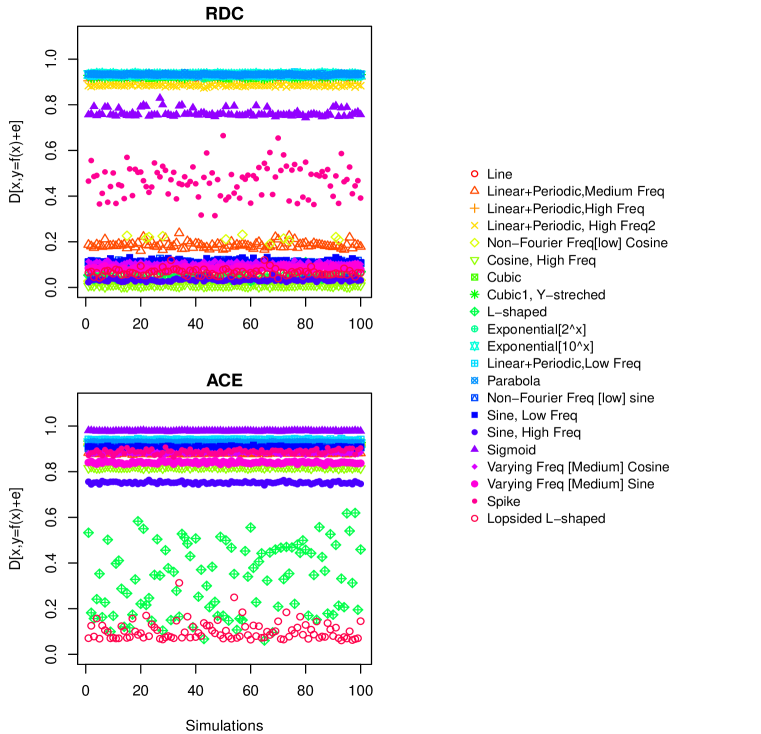
Figure 1: (color online) Equitability of ACE and RDC with mean(MSNR)=11.529, sd(MSNR)=0.233. The simulation is based on 21 types of relationship (Definitions are given in Appendix). MSNR is controlled using (5). According to the definition of equitability, they are both not equitable. In addition, RDC gives different scores to functional type ‘Spike’ in 100 simulations, and ACE gives different scores to ‘L-shaped’.

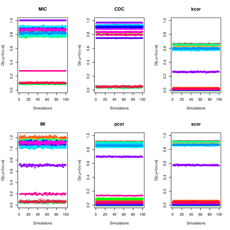
Figure 2: (color online) Equitability of MIC, MI, CDC, pcor, kcor, scor with mean(MSNR)=11.529, sd(MSNR)=0.233 (Legends are the same as that in Figure 1). The simulation is based on 21 types of functional relationships (Definitions are given in Appendix). MSNR is controlled using (5). According to the definition of equitability, these methods are not equitable. MI is equitable in a small set of functional types except four types: Sigmoid, Lopsided L-shaped, L-shaped and Spike. The performance of MIC is similar to MI, its values on these functional types except four of them are located in a small range. Especially, MIC values locate in $[0.78,0.94]$, and MI values in $[1,1.21]$.

3.3 Weak-Equitable

In this part, we discussed the weak-equitable of some popular dependence measures. In our simulation, we set MSNR ranging from 0.75 to 3. The results given in Figure 3, Figure 4, and Figure 5 show that HHG is almost power-equitable, and ACE is secondary to HHG. However ACE is sensitive to outliers, we recommend to use CDC in large data sets for association detecting.

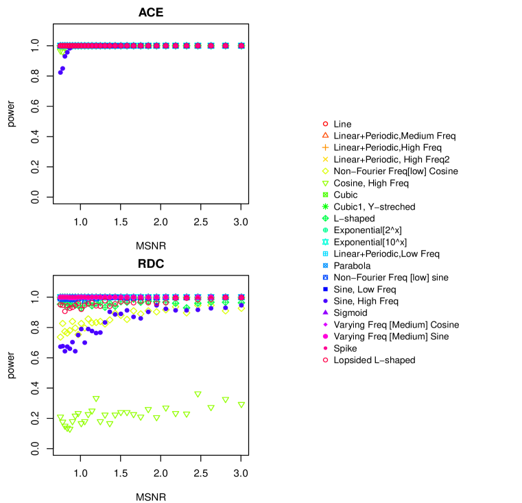
Figure 3: (color online) Weak-Equitable of ACE and RDC with mean MSNR ranges from 0.75 to 3 (Legends are the same as that in Figure 1). The simulation is based on 21 types of relationship (Definitions are given in Appendix). MSNR is controlled using (5). We can see from the results that ACE is much more equitable than RDC in this range of MSNR.

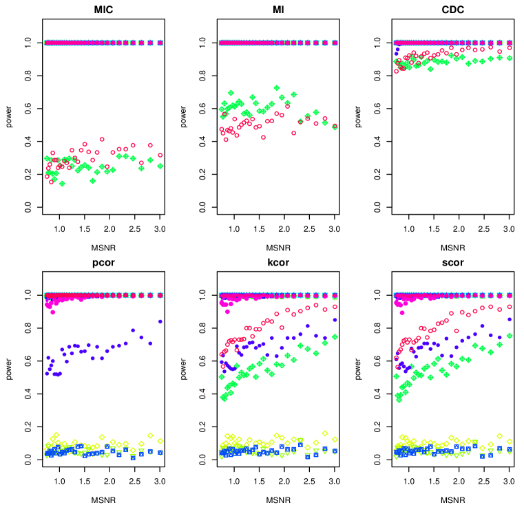
Figure 4: (color online) Weak-Equitable of MIC, MI, CDC, pcor, kcor and scor with mean MSNR range from 0.75 to 3 (Legends are the same as that in Figure 1). The simulation is based on 21 types of relationship (Definitions are given in Appendix). MSNR is controlled using (5). We can see from the results that CDC is much more equitable than others in this range of MSNR. For MI and MIC, their power-equitable property is very similar. It seems that MI is more powerful than MIC, since MI has a higher power on L-shaped and Lopsided L-shaped than MIC.

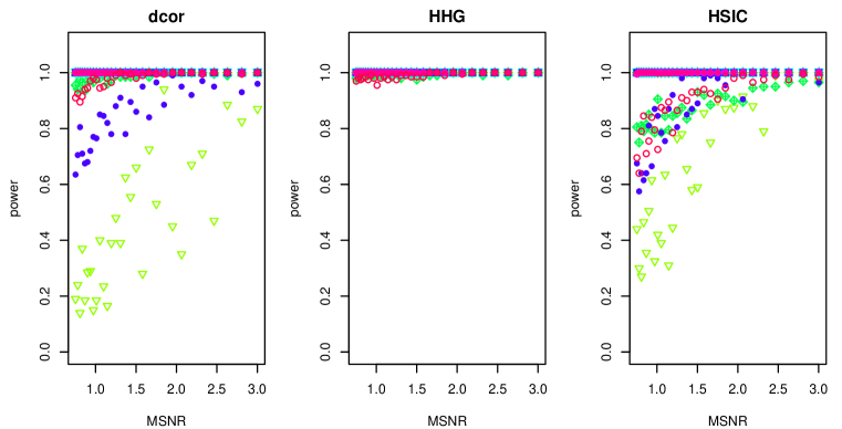
Figure 5: (color online) Weak-Equitable of dcor, HHG, and HSIC with mean MSNR range from 0.7509836 to 3.0057 (Legends are the same as that in Figure 1). The simulation is based on 21 types of relationship (Definitions are given in appendix), MSNR is controlled using (5),and simulation details are given in section 3.1. We can see from the results that HHG is much more equitable than others in that range of MSNR, here we emphasize on the range of MSNR because if there is a very small MSNR for the data, then all of the methods will have a very small power.

4 Conclusion

In this paper, we discussed the equitability and weak-equitability (power-equitability) of some common dependence measures, such as MIC, MI, dcor, CDC, ACE, RDC, HHG, Pearson correlation coefficient (pcor), Spearman rank correlation (scor), kendall’s $\tau$, and HSIC. The equitability requires a dependence measure giving similar scores to equally noisy data sets no matter what kind of functional relationship is underlying them, this requirement is so strong that it can not be satisfied by any dependence measure. Therefore, we introduced power-equitability, which only requires that all kinds of functional relationship, linear or non-linear, can be detected with the same possibility by the dependence measure. It is also called as weak-equitability because if $D$ is equitable, then it is power-equitable.

Self-equitable is the basic requirement for a dependence measure to be used as a noise measure. However, a self-equitable measure, such as MI, may not have a satisfying power in finding relationships as shown in our simulation results (see Figure 4).

Based on our simulation, we find that MI is more equitable than MIC, HHG is power-equitable, and ACE/CDC is secondary to HHG.

5 Appendix

5.1 Definition of functions

1. Line: $y=x$

2. Linear+Periodic, Low Freq: $y=0.2\sin(4(2x-1))+\frac{11}{10}(2x-1)$

3. Linear+Periodic, Medium Freq: $y=\sin(10\pi x)+x$

4. Linear+Periodic, High Freq: $y=0.1\sin(10.6(2x-1))+\frac{11}{10}(2x-1)$

5. Linear+Periodic, High Freq: $y=0.2\sin(10.6(2x-1))+\frac{11}{10}(2x-1)$

6. Non-Fourier Freq [Low] Cosine: $y=\cos(7\pi x)$

7. Cosine, High Freq: $y=\cos(14\pi x)$

8. Cubic: $y=4x^{3}+x^{2}-4x$

9. Cubi, Y-stretched: $y=41(4x^{3}+x^{2}-4x)$

10. L-shaped: $y=x/99I(x\leq\frac{99}{100})+I(x>\frac{99}{100})$

11. Exponential [$2^{x}$] : $y=2^{x}$

12. Exponential [$10^{x}$] : $y=10^{x}$

13. Parabola: $y=4x^{2}$

14. Non-Fourier Freq [Low] Sine: $y=\sin(9\pi x)$

15. Sine, Low Freq: $y=\sin(8\pi x)$

16. Sine, High Freq: $y=\sin(16\pi x)$

17. Sigmoid: $y=[50(x-0.5)+0.5]I(\frac{1}{20}\leq x\leq\frac{51}{100})+I(x>\frac{51}{100})$

18. Varying Freq [Medium] Cosine: $y=\sin(5\pi x(1+x))$

19. Varying Freq [Medium] Sine: $y=\sin(6\pi x(1+x))$

20. Spike: $y=20I(x<\frac{1}{20})+[-18x+\frac{19}{10}]I(\frac{1}{20}\leq x<\frac{1}{10})+[-\frac{x}{9}+\frac{1}{9}]I(x\geq\frac{1}{10})$

21. Lopsided L-shaped: $y=200xI(x<\frac{1}{200})+[-198x+\frac{199}{100}]I(\frac{1}{200}\leq x<\frac{1}{100})+[-\frac{x}{99}+\frac{1}{99}]I(x\geq\frac{1}{100})$

where $I(\cdot)$ is the indicator function.

References

- [1] A.Renyi. On Measures of Dependence. Acta Math.Acad.Sci. Hungar, 10:441-451, 1959.
- [2] A.Kolmogorove. Grundbegriffe der wahrcheinlichkeitsrechnung, Ergebnisse der(1933) Math.u. Grenzgebiete, Berlin
- [3] L.M.Gelfand, A.M. Jaglom and A.N.Kolmogorove,Zur allgemeinen Definition der Information. Arbeiten zur Informationstheorie, 1959, p57-60.
- [4] Gabor Szekely and Maria L.rizzo. Brownian Distance Covariance. The Annals of applied statistics 2009. Vol.3 No.4 1236-1265
- [5] Ruth Heller, Yair Heller, Malka Gorfine. A consistent multivariate test of association based on ranks of distances. arXiv:1201.3522v1.
- [6] C.E.Shannon. A mathematical theory of communication. Mobile computing and communication review, Volume5, Number1
- [7] R.Steuer, J.Kurths, C.O.Daub, J.Weise and J. Selbig,(2002) The mutual information: Detecting and evaluating dependencies between variables. BIOINFORMATICS. Vol.18 Suppl.2.S231-S240
- [8] E.H.Linfoot. An information measure of correlation. Information and Control,1(1957),p85-89
- [9] Young-I1 Moon, Balaji Rajagopalan, and Upmanu Lall. Estimation of mutual information using kernel density estimators. PHYSICAL REVIEW E. VOLUME 52. NUMBER 3. 1995.
- [10] David N.Reshef, et al. Detecting Novel Associations in Large Data Sets. Science.334,1518.
- [11] Noah Simon and Robert Tibshirani. COMMENT ON ”Detecting Novel Associations in Large Data Sets”
- [12] Trevor Hastie, Robert Tibshirani, Jerome Friedman. The Elements of Statistical Learning. Springer.2001
- [13] Delicado P, Smrekar M. Measuring non-linear dependence for two random variables distributed along a curve[J]. Statistics and Computing, 2009, 19(3): 255-269.
- [14] Yin X. Canonical correlation analysis based on information theory[J]. Journal of Multivariate Analysis, 2004, 91(2): 161-176.
- [15] Lopez-Paz, David, Philipp Hennig, and Bernhard Schlkopf. ”The randomized dependence coefficient.” Advances in Neural Information Processing Systems. 2013.
- [16] Arthur Gretton, Karsten M. Borgwardt, Malte J. Rasch, Bernhard Schlkopf, Alexander Smola. A Kernel Two-Sample Test. Journal of Machine Learning Research. 13(2012):723-773.
- [17] P czos B, Ghahramani Z, Schneider J. Copula-based kernel dependency measures[J]. arXiv preprint arXiv:1206.4682, 2012.
- [18] Renyi A. On measures of entropy and information[C]//Fourth Berkeley Symposium on Mathematical Statistics and Probability. 1961: 547-561.
- [19] Tsallis,C. Possible generalization of boltzmann-gibbs statistics. J. Statis. Phys. 52(1-2):479-487, 1988
- [20] Fernandes A D, Gloor G B. Mutual information is critically dependent on prior assumptions: would the correct estimate of mutual information please identify itself?[J]. Bioinformatics, 2010, 26(9): 1135-1139.
- [21] Khan, Shiraj; Bandyopadhyay, Sharba; Ganguly, Auroop R.; Saigal, Sunil; Erickson, David J. III; Protopopescu, Vladimir; and Ostrouchov, George, ”Relative performance of mutual information estimation methods for quantifying the dependence among short and noisy data” (2007). Civil and Environmental Engineering Faculty Publications.
- [22] Alexander Kraskov, Harald Stogbauer, and Peter Grassberger. Estimating Mutual Information.
- [23] Tan Q, Jiang H, Ding Y. Model selection method based on maximal information coefficient of residuals[J]. Acta Mathematica Scientia, 2014, 34(2): 579-592.
- [24] Nelsen R B. An introduction to copulas[M]. Springer, 1999.
- [25] Bach, Francis R. Kernel independent compoenent analysis. JMLR, 3:1-18,2002
- [26] Gretton, A., Herbrich R., and Smola, A. The kernel mutual information. In Proc. ICASSP, 2003.
- [27] Gretton,A., Bousquet, O., Smola, A. and Scholkopf, B. Measuring statistical dependence with Hilbert-Schmidt norms. In ALT, pp. 63-77, 2005.
- [28] B. Schweizer and E.F.Wolff. On nonparametric measures of dependence for random variables. The Annals of statistics, 1981, Vol.9, No.4,879-885.
- [29] Amir Dembo, Abram Kagan, Lawrence A. Shepp. Remarks on the Maximum Correlation Coefficient. Bernoulli, Vol.7, No.2 (Apr., 2001), pp. 343-350
- [30] Nickos Papadatos, Tatiana Xiafara. A simpe method for obtaining the maximal correlation coefficient and related charaterizations. Journal of Multivariate Analysis 118(2013) 102-114.
- [31] Wlodzimierz Bryc, Amir Dembo, Abram Kagan. On the maximum correlation coefficient. Technical Report No. 2002-25 August 2002.
- [32] Masashi Sugiyama, Makoto Yamada. On kernel parameter selection in Hibert-Schmidt Independent Criterion. IEICE Transactions on Information and Systems, Vol.E95-D, no.10, pp.2564-2567, 2012
- [33] Arthur Gretton, Ralf Herbrich, Alexander Smola etal. Kernel Methods for Measuring Independence. Journal of Machine Learning Research 6(2005) 2075-2129.
- [34] Dino Sejdinovic, Bharath Sriperumbudur, Arthur Gretton, Kenji Fukumizu. Equivance of distance-based and RKHS-based statistics in hypothesis testing. arXiv: arXiv:1207.6067
- [35] Charles A.Micchelli, Yuesheng Xu, Haizhang Zhang. Universal kernels. Journal of Machine Learning Reasearch 7(2006) 2651-2667.
- [36] Reshef DN, Reshef Y, Mitzenmacher M, Sabeti P (2013) Equitability analysis of the maximal information coefficient with comparisons arXiv:1301.6314v1
- [37] Justin B. Kinney and Gurinder S. Atwal Equitability, mutual information, and the maximal information coefficient PNAS 2014 111 (9) 3354-3359;
- [38] Hangjin Jiang, Yiming Ding. Dependence Measure: A comparative Study.
- [39] Reshef, David N., et al. ”Cleaning up the record on the maximal information coefficient and equitability.” Proceedings of the National Academy of Sciences 111.33 (2014): E3362-E3363.