Spontaneous symmetry breaking and inversion-line spectroscopy in gas mixtures

Abstract

According to quantum mechanics chiral molecules, that is molecules that rotate the polarization of light, should not exist. The simplest molecules which can be chiral have four or more atoms with two arrangements of minimal potential energy that are equivalent up to a parity operation. Chiral molecules correspond to states localized in one potential energy minimum and can not be stationary states of the Schrödinger equation. A possible solution of the paradox can be founded on the idea of spontaneous symmetry breaking. This idea was behind work we did previously involving a localization phase transition: at low pressure the molecules are delocalized between the two minima of the potential energy while at higher pressure they become localized in one minimum due to the intermolecular dipole-dipole interactions. Evidence for such a transition is provided by measurements of the inversion spectrum of ammonia and deuterated ammonia at different pressures. A previously proposed model gives a satisfactory account of the empirical results without free parameters. In this paper, we extend this model to gas mixtures. We find that also in these systems a phase transition takes place at a critical pressure which depends on the composition of the mixture. Moreover, we derive formulas giving the dependence of the inversion frequencies on the pressure. These predictions are susceptible to experimental test.

I Introduction

The existence of chiral molecules, that is molecules that rotate the polarization of light, has so far no universally accepted explanation. Hund was the first to point out in 1927 that such molecules according to quantum mechanics should not exist as the corresponding Hamiltonian is invariant under mirror reflection Hund . This problem became known as Hund’s paradox and was discussed in the physico-chemical literature for decades. A possible solution of the paradox can be founded on the idea of spontaneous symmetry breaking (SSB) once we take into account that the experiments deal with a large number of molecules and that their interactions are sufficient to keep them in the chiral state. This idea was behind work done previously Anderson ; jonaclaverie ; jonaclaverie2 ; Wightman ; gm ; jptprl ; Jona where the explanation of the existence was based on a localization phenomenon.

Pyramidal molecules, i.e., molecules of the kind $XY_{3}$ such as ammonia $\mathrm{NH}_{3}$, phosphine $\mathrm{PH}_{3}$, arsine $\mathrm{AsH}_{3}$, are potentially chiral. Suppose that we replace two of the hydrogens with different atoms such as deuterium and tritium: we obtain a molecule of the form $XYWZ$. This is called an enantiomer, that is a molecule whose mirror image can not be superimposed to the original one. These molecules are optically active in states where the atom X is localized on one side of the $YWZ$ plane. In the following we shall refer to potentially chiral molecules such as ammonia as pre-chiral molecules. Another example of pre-chiral molecule, not pyramidal, is deuterated disulfane $\mathrm{D}_{2}\mathrm{S}_{2}$ (see Fig. 1).

According to quantum mechanics chiral molecules should not exist as stable stationary states. Consider a pyramidal molecule $XY_{3}$. The two possible positions of the $X$ atom with respect to the plane of the $Y$ atoms are separated by a potential barrier and can be connected via tunneling. This gives rise to stationary wave functions delocalized over the two minima of the potential and of definite parity. In particular, the ground state is expected to be even under parity. Tunneling induces a doublet structure of the energy levels.

On the other hand, the existence of chiral molecules can be interpreted as a phase transition. In fact, isolated molecules do not exist in nature and the effect of the environing molecules must be taken into account. This interpretation underlies a simple mean-field model that we have developed jptprl to describe the transition of a gas of $\mathrm{NH}_{3}$ molecules from a nonpolar phase to a polar one through a localization phenomenon which gives rise to the appearance of an electric dipole moment. Even if ammonia molecules are only pre-chiral, the mechanism, as emphasized in jptprl , provides the key to understand the origin of chirality.

A quantitative discussion of the collective effects induced by coupling a molecule to the environment constituted by the other molecules of the gas was made in jonaclaverie . In this work it was shown that, due to the instability of tunneling under weak perturbations, the order of magnitude of the molecular dipole-dipole interaction may account for localized ground states. This suggested that a transition to localized states should happen when the interaction among the molecules is increased.

Evidence for such a transition was provided by measurements of the dependence of the doublet frequency under increasing pressure: the frequency vanishes for a critical pressure $P_{\mathrm{cr}}$ different for $\mathrm{NH}_{3}$ and $\mathrm{ND}_{3}$. The measurements were taken at the end of the 1940s and beginning of the 1950s Bleaney-Loubster.1948 ; Bleaney-Loubster.1950 ; Birnbaum-Maryott.1953b but no quantitative theoretical explanation was given for 50 years. Our model jptprl gives a satisfactory account of the empirical results. A remarkable feature of the model is that there are no free parameters. In particular, it describes quantitatively the shift to zero-frequency of the inversion line of $\mathrm{NH}_{3}$ and $\mathrm{ND}_{3}$ on increasing the pressure.

In this paper, we extend our model to gas mixtures. This case may be of interest, among other things, for the interpretation of the astronomical data such as those from Galileo spacecraft HSK which measured the absorption spectrum of $\mathrm{NH}_{3}$ in the Jovian atmosphere.

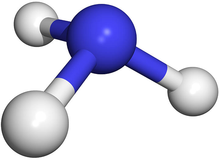
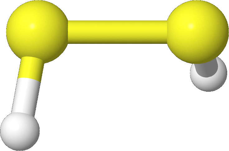
Figure 1: (Color online) Molecular structures of ammonia ($\mathrm{NH_{3}}$, left) and deuterated disulfane ($\mathrm{D_{2}S_{2}}$, right) in one of their two localized states.

The main results of this work are as follows.

(i) Also in the case of mixtures there is a quantum phase transition between a delocalized (or achiral, or nonpolar) phase and a localized (or chiral, or polar) phase. At fixed temperature, the crossover between the two phases is determined by a properly defined critical pressure $P_{\mathrm{cr}}$.

(ii) We derive formulas expressing the critical pressure of the mixture in terms of the doublet splittings of the isolated chiral molecules and the fractions of the constituents. For a binary mixture with fractions $x_{1}$ and $x_{2}$ of the two species, we have

$$\frac{1}{P_{\mathrm{cr}}}=\sum_{i=1}^{2}x_{i}\frac{1}{P^{(i)}_{\mathrm{cr}}}.$$

Supposing that species 1 is chiral, $P^{(1)}_{\mathrm{cr}}$ is the critical pressure of the pure unmixed species, namely, $P^{(1)}_{\mathrm{cr}}=\Delta E_{1}/(2\gamma_{11})$, with $\Delta E_{1}$ being the rarefied-gas doublet splitting and $\gamma_{11}$ given in terms of the temperature and other microscopic parameters, i.e., the electric dipole moment and the collision diameter of molecules 1 [see Eq. (24)]. If species 2 is non polar, then $P^{(2)}_{\mathrm{cr}}=\Delta E_{1}/(2\gamma_{12})$ with $\gamma_{12}$ expressing the polarization of molecules of species 2 by the chiral molecules of species 1 [see Eq. (10)]. If species 2 is chiral, then $P^{(2)}_{\mathrm{cr}}=\Delta E_{2}/(2\gamma_{22})$ with $\gamma_{22}$ expressing the self-consistent interaction among the molecules of species 2 [see Eq. (24)]. In both cases, the inverse critical pressure of the mixture is the fraction-weighted average of the inverse critical pressures of its components. The result is easily generalized to mixtures made up of an arbitrary number of components.

(iii) We derive formulas giving the dependence of the inversion frequencies on the pressure [see Eqs. (12) and Sec. V.2]. These results are susceptible to experimental test.

The paper is structured as follows. In the next section we briefly recall the mean-field model for a single gas of molecules exhibiting inversion doubling such as ammonia. In particular, we discuss the interaction mechanism and the strength of the interaction leading to a localization quantum phase transition with the disappearance of the inversion line. In Sec. III, we describe the well known reaction field mechanism which provides exactly the same interaction strength. The reason for arguing in terms of the reaction field is its simplicity especially in view of its extension to gas mixtures. In Sec. IV, we consider mixtures of a chiral gas with non polar molecules, such as, for instance, $\mathrm{NH}_{3}$–$\mathrm{H}_{2}$–$\mathrm{He}$. In Sec. V, we consider mixtures of chiral gases. For convenience of the reader, we have added three appendixes. They give details on the model jptprl and the comparison with the experiments Bleaney-Loubster.1948 ; Bleaney-Loubster.1950 ; Birnbaum-Maryott.1953b .

II Chiral molecules as a case of spontaneous symmetry breaking

We model a gas of pre-chiral, e.g., pyramidal, molecules as a set of two-level quantum systems, that mimic the inversion degree of freedom of an isolated molecule, mutually interacting via the dipole-dipole electric force.

The Hamiltonian for the single isolated molecule is assumed of the form $-\sigma^{x}\Delta E/2$, where $\Delta E$ is the inversion energy splitting measured in a rarefied gas of the considered species and

$$\sigma^{x}=\left(\begin{array}[]{cc}0&1\\ 1&0\end{array}\right)$$

is the Pauli matrix with symmetric and antisymmetric delocalized tunneling eigenstates $\varphi_{+}$ and $\varphi_{-}$:

$$\varphi_{+}=\frac{1}{\sqrt{2}}\left(\begin{array}[]{c}1\\ 1\end{array}\right),\qquad\varphi_{-}=\frac{1}{\sqrt{2}}\left(\begin{array}[]{c}\phantom{-}1\\ -1\end{array}\right).$$

Since the rotational degrees of freedom of an isolated molecule are faster than the inversion ones, on the time scales of the inversion dynamics, namely, $\hbar/\Delta E$, the molecules in a gas feel an attraction arising from the angle averaging of the effective dipole-dipole interaction at the actual temperature of the gas Keesom . The localizing effect of the dipole-dipole interaction between two molecules $i$ and $j$ can be represented by an interaction term of the form $-\mathfrak{g}_{ij}\sigma^{z}_{i}\otimes\sigma^{z}_{j}$, with $\mathfrak{g}_{ij}>0$, where

$$\sigma^{z}=\left(\begin{array}[]{cc}1&\phantom{-}0\\ 0&-1\end{array}\right)$$

is the Pauli matrix with left and right localized eigenstates $\varphi_{L}$ and $\varphi_{R}$

$$\varphi_{L}=\left(\begin{array}[]{c}1\\ 0\end{array}\right),\qquad\varphi_{R}=\left(\begin{array}[]{c}0\\ 1\end{array}\right).$$

The Hamiltonian for $N$ interacting molecules then reads as

$$H=-\frac{\Delta E}{2}\sum_{i=1}^{N}\sigma^{x}_{i}-\sum_{i=1}^{N}\sum_{j=i+1}^{N}\mathfrak{g}_{ij}\,\sigma^{z}_{i}\otimes\sigma^{z}_{j}.$$ (1)

For a gas of moderate density, we approximate the behavior of the $N\gg 1$ molecules with the mean-field Hamiltonian

$$h(\psi)=-\frac{\Delta E}{2}\sigma^{x}-\frac{G}{N}\langle\psi,\sigma^{z}\psi\rangle\sigma^{z},$$ (2)

where $\psi$ is the mean-field molecular state to be determined self-consistently by solving the nonlinear eigenvalue problem associated with Eq. (2) and the normalization condition $\langle\psi,\psi\rangle=N$. The scalar product between two Pauli spinors $\psi$ and $\phi$ is defined in terms of their two components in the standard way

$$\langle\psi,\phi\rangle=\overline{\psi}_{1}\phi_{1}+\overline{\psi}_{2}\phi_{2}.$$

The parameter $G$ accounts for the effective dipole interaction energy of a single molecule with the rest of the gas. It must be identified with a sum over all possible molecular distances and all possible dipole orientations calculated assuming that, concerning the translational, vibrational, and rotational degrees of freedom, the $N$ molecules behave as an ideal gas at thermal equilibrium at temperature $T$. This assumption relies on a sharp separation (decoupling) between these degrees of freedom and the inversion motion Townes-Schawlow .

We now discuss the calculation of $G$ following Keesom Keesom . An alternative derivation of $G$ will be shown later based on the so called reaction field mechanism.

Let us define an effective interaction potential $V(r)$ between two electric dipoles at distance $r$ via the formula

$$e^{-V(r)/k_{B}T}=\langle e^{-V(r,\boldsymbol{\mu}_{1},\boldsymbol{\mu}_{2})/k_{B}T}\rangle,$$

where

$$V(r,\boldsymbol{\mu}_{1},\boldsymbol{\mu}_{2})=\frac{\boldsymbol{\mu}_{1}\cdot\boldsymbol{\mu}_{2}-3(\boldsymbol{\mu}_{1}\cdot\boldsymbol{r})(\boldsymbol{r}\cdot\boldsymbol{\mu}_{2})r^{-2}}{4\pi\varepsilon_{0}r^{3}}$$

is the standard dipole-dipole interaction potential and $\langle\dots\rangle$ denotes the average over all possible orientations of the vectors $\boldsymbol{\mu}_{1}$ and $\boldsymbol{\mu}_{2}$. Assuming that $V(r)\ll k_{B}T$ and observing that $\langle V(r,\boldsymbol{\mu}_{1},\boldsymbol{\mu}_{2})\rangle=0$, we approximately evaluate the effective potential as

$$V(r) =-\frac{1}{2}\left\langle\left(\frac{V(r,\boldsymbol{\mu}_{1},\boldsymbol{\mu}_{2})}{k_{B}T}\right)^{2}\right\rangle k_{B}T$$

$$=-\frac{\mu_{1}^{2}\mu_{2}^{2}}{3(4\pi\varepsilon_{0})^{2}k_{B}Tr^{6}}.$$

In the case of a gas of molecules with dipole moments $\mu$, the effective interaction energy of one molecule with the rest of the gas amounts to $-G$, where

$$G =\int_{d}^{\infty}\rho(r)\frac{\mu^{4}}{3(4\pi\varepsilon_{0})^{2}k_{B}Tr^{6}}4\pi r^{2}\mathrm{d}{r}$$

$$=\frac{4\pi}{9}\frac{\mu^{4}P}{(4\pi\varepsilon_{0}k_{B}T)^{2}d^{3}}.$$ (3)

To get the above result we used $\rho(r)=P/k_{B}T$, the ideal gas density at pressure $P$ and temperature $T$. Note that $d$ is the minimal distance at which two molecules can be found, namely, the so called molecular collision diameter. At fixed temperature, the effective interaction constant $G$ increases linearly with the gas pressure $P$.

The nonlinear eigenvalue problem associated with Eq. (2) is solved in detail in Appendix A. There exists a critical value of the interaction strength, $G_{\mathrm{cr}}=\Delta E/2$, such that for $G<G_{\mathrm{cr}}$ the mean-field eigenstate with minimal energy is $\psi=\sqrt{N}\varphi_{+}$, with delocalized molecules, whereas for $G>G_{\mathrm{cr}}$ there are two degenerate states of minimal energy. These are chiral states transformed into each other by the parity operator $\sigma^{x}$ approaching the localized states $\varphi_{L},\varphi_{R}$ for $G\gg G_{\mathrm{cr}}$. We thus have a quantum phase transition between a delocalized (or achiral, or nonpolar) phase and a localized (or chiral, or polar) phase. In view of the dependence of $G$ on $P$, we can define a critical pressure at which the phase transition takes place

$$P_{\mathrm{cr}}=\frac{9}{8\pi}\frac{\Delta Ed^{3}(4\pi\varepsilon_{0}k_{B}T)^{2}}{\mu^{4}}.$$ (4)

In Table 1 we report the values of $P_{\mathrm{cr}}$ calculated for different pre-chiral molecules.

Table 1: Rarefied-gas energy splitting $\Delta E$, electric dipole moment $\mu$, and collision diameter $d$ measured for different pre-chiral molecules Townes-Schawlow ; HCP . In the fourth column, we report the critical pressure $P_{\mathrm{cr}}$ evaluated by Eq. (4) at $T=300$ K.

	$\Delta E$ (cm-1)	$\mu$ (Debye)	$d$ (Å)	$P_{\mathrm{cr}}$ (atm)
$\mathrm{NH_{3}}$	0.81	1.47	4.32	1.69
$\mathrm{ND_{3}}$	0.053	1.47	4.32	0.11
$\mathrm{D_{2}S_{2}}$	$10^{-9}$	1.56	5.97	$4.3\times 10^{-9}$

In Appendix B we show that in the delocalized phase the inversion angular frequency of the interacting molecules depends on the pressure as

$$\hbar\overline{\omega}=\Delta E\sqrt{1-\frac{P}{P_{\mathrm{cr}}}}.$$ (5)

This formula is interesting as it expresses the ratio of two microscopic quantities, $\hbar\overline{\omega}$ and $\Delta E$, as a universal function of the ratio of the macroscopic variables $P$ and $P_{\mathrm{cr}}$. Furthermore, it provides a very good representation of some spectroscopic data, namely, the shift to zero frequency of the inversion line of $\mathrm{NH}_{3}$ or $\mathrm{ND}_{3}$, as it appears from Fig. 11, see Appendix C for more details.

III The reaction field mechanism

The mean-field coupling constant $G$ introduced in Section II can be estimated, obtaining the same result, using a different argument which can be easily generalized. This is the reaction field mechanism widely used in physics and chemistry Onsager ; Bottcher .

Let us consider a spherical cavity of radius $a$ in a homogeneous dielectric medium characterized by a relative dielectric constant $\varepsilon_{r}$. An electric dipole $\boldsymbol{\mu}$ placed at the center of the cavity polarizes the dielectric medium inducing inside the sphere a reaction field $\boldsymbol{R}$ proportional to $\boldsymbol{\mu}$:

$$\boldsymbol{R}=\frac{2(\varepsilon_{r}-1)}{2\varepsilon_{r}+1}\frac{\boldsymbol{\mu}}{4\pi\varepsilon_{0}a^{3}}.$$

As a result, the dipole acquires an energy

$$\mathscr{E}=-\frac{1}{2}\boldsymbol{\mu}\cdot\boldsymbol{R}=-\frac{\varepsilon_{r}-1}{2\varepsilon_{r}+1}\frac{\mu^{2}}{4\pi\varepsilon_{0}a^{3}}.$$ (6)

By using the Clausius–Mossotti relation

$$\frac{\varepsilon_{r}-1}{\varepsilon_{r}+2}=\frac{1}{3}\rho\left(\alpha+\alpha^{\mathrm{D}}\right),$$

where $\alpha$ is the molecular polarizability and $\alpha^{\mathrm{D}}=\mu^{2}/(3\varepsilon_{0}k_{B}T)$ is the Debye (orientation) polarizability, and observing that for a chiral gas $\alpha^{\mathrm{D}}\gg\alpha$ (for instance, in the case of $\mathrm{NH}_{3}$ we have $\alpha\simeq 2~{}\mbox{\AA}^{3}$ whereas $\alpha^{\mathrm{D}}\simeq 217~{}\mbox{\AA}^{3}$ at $T=300~{}\mathrm{K}$), we get

$$\mathscr{E}=-\frac{4\pi}{9}\frac{\mu^{4}P}{(4\pi\varepsilon_{0}k_{B}T)^{2}a^{3}}.$$

In all the above expressions we have $\varepsilon_{r}\simeq 1$ so that we approximated $\varepsilon_{r}+2\simeq 2\varepsilon_{r}+1\simeq 3$.

We exactly have $\mathscr{E}=-G$ provided $a=d$, where $d$ is the molecular collision diameter introduced in Eq. (II) as the minimum distance between two interacting molecules. In fact, the size of the spherical cavity is not arbitrary. Microscopic arguments Hynne-Bullough ; Linder show that $a$ must be identified with the radius of an effective hard core, namely, the molecular collision diameter $d$.

IV Mixtures of a chiral gas with non polar molecules

By using the reaction field approach to the coupling constant $G$, we now generalize the mean-field model of Section II to the case of a mixture of chiral with non polar molecules. Consider a gas mixture of two species labeled 1 and 2. In this case, the Clausius-Mossotti relation reads as

$$\frac{\varepsilon_{r}-1}{\varepsilon_{r}+2}=\frac{1}{3}\left(\rho_{1}\left(\alpha_{1}+\alpha^{\mathrm{D}}_{1}\right)+\rho_{2}\left(\alpha_{2}+\alpha^{\mathrm{D}}_{2}\right)\right).$$

If species $1$ is pre-chiral, i.e., polar, $\alpha_{1}$ can be neglected with respect to $\alpha^{\mathrm{D}}_{1}$ and if species $2$ is non polar $\alpha^{\mathrm{D}}_{2}=0$. The energy acquired by one molecule of the polar species, having electric dipole moment $\mu_{1}$, then is

$$\mathscr{E}_{1}=-\frac{1}{3}\rho_{1}\alpha^{\mathrm{D}}_{1}\frac{\mu_{1}^{2}}{4\pi\varepsilon_{0}d_{11}^{3}}-\frac{1}{3}\rho_{2}\alpha_{2}\frac{\mu_{1}^{2}}{4\pi\varepsilon_{0}d_{12}^{3}},$$ (7)

where $d_{11}$ and $d_{12}$ are the diameters of the molecular collisions $1$-$1$ and $1$-$2$, namely, $d_{11}=2r_{1}$ and $d_{12}=r_{1}+r_{2}$, $r_{1}$ and $r_{2}$ being the hard sphere radii of the molecules 1 and 2. If the density $\rho_{1}$ is such that $\rho_{1}\alpha^{\mathrm{D}}_{1}\ll\rho_{2}\alpha_{2}$, the above formula reduces to

$$\mathscr{E}_{1}=-\frac{1}{3}\rho_{2}\alpha_{2}\frac{\mu_{1}^{2}}{4\pi\varepsilon_{0}d_{12}^{3}}.$$

This formula approximates the case of a single polar molecule immersed in a non polar gas.

For a mixture of chiral and non polar molecules, the mean-field molecular state of the chiral species 1, $\psi_{1}$, is determined similarly to the case of a single chiral gas. The only degree of freedom of the non polar molecules is the deformation which, in turn, is proportional to the electric dipole moment of the chiral molecules. Therefore, we assume the following nonlinear Hamiltonian similar to Eq. (2)

$$h_{1}(\psi_{1})=-\frac{\Delta E_{1}}{2}\sigma_{1}^{x}-\frac{G_{1}}{N_{1}}\langle\psi_{1},\sigma_{1}^{z}\psi_{1}\rangle\sigma_{1}^{z}.$$ (8)

The mean-field molecular state $\psi_{1}$ is normalized to the number of molecules of the species 1, namely, $\langle\psi_{1},\psi_{1}\rangle=N_{1}$. The parameter $G_{1}$ accounts for the effective dipole interaction energy of a single chiral molecule with the rest of the gas constituted by polar and non polar species. According to the reaction field arguments, we have just to identify $G_{1}=-\mathscr{E}_{1}$, where $\mathscr{E}_{1}$ is given by Eq. (7). Thus we see that $G_{1}$ is the sum of two contributions

$$G_{1}=G_{11}+G_{12},$$

where

$$G_{11}=\frac{4\pi}{9}\frac{\mu_{1}^{4}P_{1}}{(4\pi\varepsilon_{0}k_{B}T)^{2}d_{11}^{3}}=\gamma_{11}P_{1}$$ (9)

is the energy provided by the interaction with the chiral species and

$$G_{12}=\frac{1}{3}\frac{\alpha_{2}\mu_{1}^{2}P_{2}}{4\pi\varepsilon_{0}k_{B}Td_{12}^{3}}=\gamma_{12}P_{2}$$ (10)

the energy due to the presence of the non polar molecules. In the above expressions we used the ideal gas relations $\rho_{1}=P_{1}/k_{B}T$ and $\rho_{2}=P_{2}/k_{B}T$, $P_{1}$ and $P_{2}$ being the partial pressures of the species 1 and 2.

The analysis of the mean-field Hamiltonian (8) is identical to the case of a single chiral gas. We have a localization phase transition when $G_{1}$ becomes equal to ${G_{1}}_{\mathrm{cr}}=\Delta E_{1}/2$. The transition can be considered as a function of the total pressure $P=P_{1}+P_{2}$ of the mixture and of the fractions of the two species $x_{1}=P_{1}/P$ and $x_{2}=P_{2}/P$. In this case, an important prediction is that, instead of a unique critical pressure, we have a critical line parametrized by $x_{1}$ (or $x_{2}=1-x_{1}$):

$$P_{\mathrm{cr}}(x_{1})=\frac{\Delta E_{1}}{2x_{1}\gamma_{11}+2(1-x_{1})\gamma_{12}},$$ (11)

where $\gamma_{11}=G_{11}/P_{1}$ and $\gamma_{12}=G_{12}/P_{2}$ with $G_{11}$ and $G_{12}$ as in Eqs. (9) and (10).

The inversion frequency of the chiral species 1 can be evaluated as in the case of a single chiral gas. The result is formally identical to that in Eq. (5),

$$\hbar\overline{\omega}_{1}=\Delta E_{1}\sqrt{1-\frac{P}{P_{\mathrm{cr}}(x_{1})}},$$ (12)

with the angular frequency $\overline{\omega}_{1}$ which is now a function of the pressure $P$ of the mixture and of the fraction $x_{1}$ of the chiral species. However, for any fixed value of $x_{1}$, the ratio $\hbar\overline{\omega}_{1}/\Delta E_{1}$ is still a universal function of $P/P_{\mathrm{cr}}$ independent of the nature of species 1.

In Fig. 2, we show the variation of the critical pressure as a function of the fraction $x$ of the chiral species for the mixtures NH₃–He and D₂S₂–He. The value of $P_{\mathrm{cr}}$ at $x=1$ coincides with that reported in Table 1 for a pure chiral gas, whereas for $x\to 0$ the critical pressure approaches a much higher value. The ratio

$$\frac{\lim_{x\to 0}P_{\mathrm{cr}}(x)}{P_{\mathrm{cr}}(1)}=\frac{4\pi}{3}~{}\frac{\mu_{1}^{2}/(4\pi\varepsilon_{0}d_{11}^{3})}{k_{B}T}~{}\frac{d_{12}^{3}}{\alpha_{2}}$$

amounts to about 400 in the examples of Fig. (2).

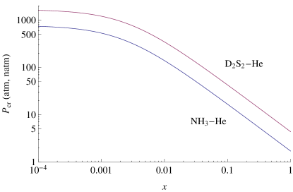
Figure 2: (Color online) Critical pressure $P_{\mathrm{cr}}$ as a function of the chiral species fraction $x$ for NH₃–He (bottom) and D₂S₂–He (top) mixtures at $T=300$ K. Note that pressure units are atm in the case of NH₃–He and natm in the case of D₂S₂–He.

The above analysis is immediately generalized to a mixture containing one chiral gas and an arbitrary number of non polar gases. As an example, for a ternary mixture (as before, species 1 is the chiral one) we have a surface of critical pressures

$$P_{\mathrm{cr}}(x_{1},x_{2})=\frac{\Delta E_{1}}{2x_{1}\gamma_{11}+2x_{2}\gamma_{12}+2(1-x_{1}-x_{2})\gamma_{13}},$$

where $\gamma_{13}=G_{13}/P_{3}$ with $G_{13}$ given by an expression analogous to Eq. (10). This term expresses the polarization of the molecules of species 3 by the chiral molecules of species 1.

The above results may be of interest, among other things, in the interpretation of astronomical data such as those from Galileo spacecraft HSK which measured the absorption spectrum of NH₃ in the Jovian atmosphere. Note that, since the atmosphere of Jupiter is mostly made of molecular hydrogen and helium in roughly solar proportions whereas ammonia has a tiny fraction, the critical pressure of the mixture is drastically different if compared with the $1.69~{}\mathrm{atm}$ value of ammonia. For fractions $x_{\mathrm{NH}_{3}}\simeq 0.01$, $x_{\mathrm{H}_{2}}\simeq 0.86$ and $x_{\mathrm{He}}\simeq 0.13$, we estimate $P_{\mathrm{cr}}$ ranging from $15~{}\mathrm{atm}$ at $T=100~{}\mathrm{K}$ to $165~{}\mathrm{atm}$ at $T=400~{}\mathrm{K}$. This implies that no ammonia inversion line shift can be observed in microwave absorption measurements performed in the atmosphere of Jupiter.

V Mixtures of chiral gases

It is possible to extend our mean-field approach to gas mixtures made of several chiral species. We start considering the simplest case of two species.

In Sec. V.1, we illustrate the model and evaluate the stationary molecular states of the mixture. In a first reading, one can skip the discussion after Eq. (18) and look at the results summarized in Table 2. As in the case of a single chiral gas, the mixture undergoes a localization phase transition at a critical pressure $P_{\mathrm{cr}}$. For $0<P<P_{\mathrm{cr}}$, the lowest-energy molecular state of the mixture, named $d_{++}$, corresponds to molecules of both species in a delocalized symmetric configuration. For $P>P_{\mathrm{cr}}$, new minimal-energy molecular states appear with twofold degeneracy. These states, named $c_{LL}$ and $c_{RR}$, correspond to molecules of both species in a chiral configuration of type $L$ or $R$. Equation (25) provides a simple formula for $P_{\mathrm{cr}}$. The inverse critical pressure of the mixture is the fraction-weighted average of the inverse critical pressures of its components.

In Sec. V.2, we evaluate the excitation energies of a two-species mixture by using the linear-response theory. The results are summarized by Eq. (43). We have two normal modes which at low pressure reduce to the inversion of the component species. By increasing the pressure, the energy of both modes decreases, the smaller one vanishing at $P=P_{\mathrm{cr}}$, the larger one approaching for $P\gg P_{\mathrm{cr}}$ the asymptotic value given by Eq. (44). An example of this behavior is shown in Figs. 5 and 6 in the case of a $\mathrm{NH}_{3}$–$\mathrm{ND}_{3}$ mixture.

Finally, in Sec. V.3, we discuss the consistency of the developed theory by considering the absorption coefficient and two limits in which it must reduce to that of a single chiral gas, namely, the limit of zero fraction of one species and the limit of equal species. We also discuss the possibility of experimental tests for the considered $\mathrm{NH}_{3}$–$\mathrm{ND}_{3}$ mixture.

All the above results can be generalized to mixtures of several chiral gases.

V.1 Molecular states

For a mixture of two chiral gases, the Clausius-Mossotti relation reads as

$$\frac{\varepsilon_{r}-1}{\varepsilon_{r}+2}=\frac{1}{3}\left(\rho_{1}\alpha^{\mathrm{D}}_{1}+\rho_{2}\alpha^{\mathrm{D}}_{2}\right),$$

where the Debye polarizations $\alpha_{i}^{\mathrm{D}}=\mu_{i}^{2}/(3\varepsilon_{0}k_{B}T)$, $i=1,2$, are given in terms of the molecular electric-dipole moments, $\mu_{1}$ and $\mu_{2}$, of the two species. According to Eq. (6), due to mutual interactions the molecules of species 1 and 2 acquire the energies

$$\mathscr{E}_{1}=-\frac{4\pi}{9}\frac{\mu_{1}^{2}\mu_{1}^{2}Px_{1}}{(4\pi\varepsilon_{0}k_{B}T)^{2}d_{11}^{3}}-\frac{4\pi}{9}\frac{\mu_{1}^{2}\mu_{2}^{2}Px_{2}}{(4\pi\varepsilon_{0}k_{B}T)^{2}d_{11}^{3}},$$

$$\mathscr{E}_{2}=-\frac{4\pi}{9}\frac{\mu_{2}^{2}\mu_{2}^{2}Px_{2}}{(4\pi\varepsilon_{0}k_{B}T)^{2}d_{22}^{3}}-\frac{4\pi}{9}\frac{\mu_{2}^{2}\mu_{1}^{2}Px_{1}}{(4\pi\varepsilon_{0}k_{B}T)^{2}d_{22}^{3}}.$$

As usual, we used the ideal gas relations $\rho_{i}=P_{i}/k_{B}T$, $i=1,2$, and introduced the fractions $x_{1}=P_{1}/P$ and $x_{2}=P_{2}/P$, where $P$ is the total pressure of the mixture.

We describe the inversion degrees of freedom of the two species by mean-field molecular states $\psi_{1},\psi_{2}$ normalized to the number of molecules of the corresponding species, $\langle\psi_{1},\psi_{1}\rangle=N_{1}$, $\langle\psi_{2},\psi_{2}\rangle=N_{2}$. Here, $\psi_{1}$ and $\psi_{2}$ are Pauli spinors and the scalar product is defined as in Section II. By writing $\mathscr{E}_{i}=-\sum_{j=1}^{2}G_{i,j}$, $i=1,2$, where

$$G_{ij}=\frac{4\pi}{9}\frac{\mu_{i}^{2}\mu_{j}^{2}Px_{j}}{(4\pi\varepsilon_{0}k_{B}T)^{2}d_{ii}^{3}},$$ (13)

and reasoning as in Sec. II, we introduce the following set of two nonlinear Hamiltonians:

$$h_{1}(\psi_{1},\psi_{2}) =-\frac{\Delta E_{1}}{2}\sigma_{1}^{x}-\sum_{j=1}^{2}\frac{G_{1j}}{N_{j}}\langle\psi_{j},\sigma_{j}^{z}\psi_{j}\rangle\sigma_{1}^{z},$$ (14a)

$$h_{2}(\psi_{1},\psi_{2}) =-\frac{\Delta E_{2}}{2}\sigma_{2}^{x}-\sum_{j=1}^{2}\frac{G_{2j}}{N_{j}}\langle\psi_{j},\sigma_{j}^{z}\psi_{j}\rangle\sigma_{2}^{z}.$$ (14b)

Pauli operators now have a label $i=1,2$ relative to the species they refer to. Stationary states are obtained by solving the eigenvalue problem

$$h_{1}(\psi_{1},\psi_{2})\psi_{1} =\lambda_{1}\psi_{1},$$ (15a)

$$h_{2}(\psi_{1},\psi_{2})\psi_{2} =\lambda_{2}\psi_{2},$$ (15b)

where $\lambda_{1},\lambda_{2}$ are the Lagrange multipliers associated with the conservation of the particle number of species 1 and 2, separately. In fact, the molecules of the two species can not be transformed into each another.

As discussed in the case of a single chiral gas (see Appendix A) the molecules of the species 1 and 2 will occupy the eigenstate having the lowest energy

$$\mathcal{E}(\psi_{1},\psi_{2})= -\sum_{i=1}^{2}\frac{\Delta E_{i}}{2}\langle\psi_{i},\sigma_{i}^{x}\psi_{i}\rangle$$

$$-\sum_{i=1}^{2}\sum_{j=1}^{2}\frac{G_{ij}}{2N_{j}}\langle\psi_{i},\sigma_{i}^{z}\psi_{i}\rangle\langle\psi_{j},\sigma_{j}^{z}\psi_{j}\rangle.$$ (16)

In virtue of the symmetry property $G_{12}/N_{2}=G_{21}/N_{1}$, the above energy is a constant of motion of the infinite-dimensional Hamiltonian system

$$i\hbar\frac{\mathrm{d}}{\mathrm{d}{t}}\psi_{1}=h_{1}(\psi_{1},\psi_{2})\psi_{1},$$

$$i\hbar\frac{\mathrm{d}}{\mathrm{d}{t}}\psi_{2}=h_{2}(\psi_{1},\psi_{2})\psi_{2}.$$

Notice, in fact, that $\delta\mathcal{E}(\psi_{1},\psi_{2})/\delta\overline{\psi}_{i}=h_{i}(\psi_{1},\psi_{2})\psi_{i}$.

To solve the eigenvalue problem (15), we write

$$\psi_{i}=a_{i}\varphi_{+}^{(i)}+b_{i}\varphi_{-}^{(i)},\qquad i=1,2.$$ (18)

The coefficients $a_{i}$ and $b_{i}$ can be chosen real and are normalized to the number of molecules of each species, $a_{i}^{2}+b_{i}^{2}=N_{i}$. Up to an irrelevant global sign, we can also choose $a_{1}$ and $a_{2}$ non-negative. By inserting the expressions (18) into Eq. (15), we find that $a_{1},b_{1},a_{2},b_{2}$ are the solutions of the system of equations

$$\Delta E_{i}a_{i}b_{i}=\sum_{j=1}^{2}2g_{ij}\left(a_{i}^{2}-b_{i}^{2}\right)a_{j}b_{j},\qquad i=1,2,$$ (19)

where $g_{ij}=G_{ij}/N_{j}$. Once a solution of this system is found, the corresponding energy can be evaluated as

$$\mathcal{E}=-\sum_{i=1}^{2}\frac{\Delta E_{i}}{2}\left(a_{i}^{2}-b_{i}^{2}\right)-\sum_{i=1}^{2}\sum_{j=1}^{2}2g_{ij}a_{i}b_{i}a_{j}b_{j}.$$

It is convenient to discuss the solutions of Eq. (19) in function of the parameter $P\in[0,\infty)$. In fact, the matrix elements $g_{ij}$ are proportional to the pressure. For any value of $P$, Eq. (19) admits solutions such that $a_{1}b_{1}=0$ and $a_{2}b_{2}=0$. There are four different solutions satisfying this condition and the normalization rule (see Table 2). The solution

$$a_{1}=\sqrt{N_{1}},\quad b_{1}=0,\quad a_{2}=\sqrt{N_{2}},\quad b_{2}=0$$ (20)

is that with the lowest energy $\mathcal{E}=-N(x_{1}\Delta E_{1}/2+x_{2}\Delta E_{2}/2)$. We name this solution $d_{++}$ because it corresponds to molecules of both species in a delocalized symmetric configuration.

Table 2: Stationary molecular states for a mixture of two chiral gases with fractions $x_{1}=N_{1}/N$ and $x_{2}=N_{2}/N$, $N=N_{1}+N_{2}$ being the total number of molecules. The states are classified in column 1 as delocalized ($d$) even ($+$) or odd ($-$) and chiral ($c$) left ($L$) or right ($R$). This classification results from the decomposition of the two-species molecular states in terms of the delocalized eigenfunctions of $\sigma^{x}$ via the coefficients $a_{1},b_{1},a_{2},b_{2}$ as in Eq. (18). The values of $a_{1},b_{1},a_{2},b_{2}$ are found by solving Eq. (19) with the normalization conditions $a_{1}^{2}+b_{1}^{2}=N_{1}$ and $a_{2}^{2}+b_{2}^{2}=N_{2}$. The chiral solutions exist only for $P>P_{\mathrm{cr}}$ and are defined in terms of two parameters $q_{1}$ and $q_{2}$ shown in Fig. 4. The energy per unit molecule associated with each state [see Eq. (16)] is reported in the last column. For $P<P_{\mathrm{cr}}$ the solution of minimal energy is $d_{++}$ while for $P>P_{\mathrm{cr}}$ there are two degenerate solutions of minimal energy, namely, $c_{LL}$ and $c_{RR}$. Other higher-energy states bifurcating at pressures larger than $P_{\mathrm{cr}}$, see Fig. 3, are not reported in this table.

	$a_{1}$	$b_{1}$	$a_{2}$	$b_{2}$	$\mathcal{E}/N$
d++	$\sqrt{N_{1}}$	0$\sqrt{\frac{A_{B}}{C}}$	$\sqrt{N_{2}}$	0	$-\frac{x_{1}\Delta E_{1}}{2}-\frac{x_{2}\Delta E_{2}}{2}$
d+-	$\sqrt{N_{1}}$	0$\sqrt{\frac{A_{B}}{C}}$	0	$\sqrt{N_{2}}$	$-\frac{x_{1}\Delta E_{1}}{2}+\frac{x_{2}\Delta E_{2}}{2}$
d-+	0$\sqrt{\frac{A_{B}}{C}}$	$\sqrt{N_{1}}$	$\sqrt{N_{2}}$	0	$+\frac{x_{1}\Delta E_{1}}{2}-\frac{x_{2}\Delta E_{2}}{2}$
d–	0$\sqrt{\frac{A_{B}}{C}}$	$\sqrt{N_{1}}$	0	$\sqrt{N_{2}}$	$+\frac{x_{1}\Delta E_{1}}{2}+\frac{x_{2}\Delta E_{2}}{2}$
cLL	$\sqrt{\frac{N_{1}}{2}(1+q_{1})}$	$\sqrt{\frac{N_{1}}{2}(1-q_{1})}$	$\sqrt{\frac{N_{2}}{2}(1+q_{2})}$	$\sqrt{\frac{N_{2}}{2}(1-q_{2})}$	$-\sum_{i}\frac{x_{i}q_{i}\Delta E_{i}}{2}-\sum_{i,j}\frac{x_{i}x_{j}\sqrt{1-q_{i}^{2}}\sqrt{1-q_{j}^{2}}\gamma_{ij}P}{2}$
cRR	$\sqrt{\frac{N_{1}}{2}(1+q_{1})}$	$-\sqrt{\frac{N_{1}}{2}(1-q_{1})}$	$\sqrt{\frac{N_{2}}{2}(1+q_{2})}$	$-\sqrt{\frac{N_{2}}{2}(1-q_{2})}$	$-\sum_{i}\frac{x_{i}q_{i}\Delta E_{i}}{2}-\sum_{i,j}\frac{x_{i}x_{j}\sqrt{1-q_{i}^{2}}\sqrt{1-q_{j}^{2}}\gamma_{ij}P}{2}$

If $a_{1}b_{1}=0$ and $a_{2}b_{2}\neq 0$ or, vice versa, $a_{1}b_{1}\neq 0$ and $a_{2}b_{2}=0$, Eq. (19) has no solutions. In fact, if $a_{1}b_{1}=0$ then $a_{1}^{2}-b_{1}^{2}=\pm N_{1}$ and Eq. (19) for $i=1$ gives $0=\pm 2g_{12}N_{1}a_{2}b_{2}$ which can not be solved for $a_{2}b_{2}\neq 0$.

Equation (19) admits solutions with $a_{1}b_{1}\neq 0$ and $a_{2}b_{2}\neq 0$ if and only if

$$\left[\Delta E_{1}-2g_{11}(a_{1}^{2}-b_{1}^{2})\right]\left[\Delta E_{2}-2g_{22}(a_{2}^{2}-b_{2}^{2})\right]$$

$$\qquad-4g_{12}g_{21}(a_{1}^{2}-b_{1}^{2})(a_{2}^{2}-b_{2}^{2})=0.$$ (21)

In fact, think of Eq. (19) as a linear homogeneous system of equations in the two unknowns $a_{1}b_{1}$ and $a_{2}b_{2}$. This system admits a nontrivial solution $(a_{1}b_{1},a_{2}b_{2})\neq(0,0)$ if and only if its determinant is 0, namely, Eq. (21). Any non trivial solution is necessarily of the form $a_{1}b_{1}\neq 0$ and $a_{2}b_{2}\neq 0$ because we have already established that Eq. (19) does not have solutions with just one term between $a_{1}b_{1}$ and $a_{2}b_{2}$ equal to 0.

If $(a_{1},b_{1},a_{2},b_{2})$ is a solution of Eq. (19), that is true also for $(a_{1},-b_{1},a_{2},-b_{2})$ and these two solutions have the same energy. Therefore, each eigenstate obtained for $a_{1}b_{1}\neq 0$ and $a_{2}b_{2}\neq 0$ has a twofold degeneracy.

Observing that $g_{11}g_{22}-g_{12}g_{21}=0$, Eq. (21) can be rewritten as

$$4g_{11}a_{1}^{2}\Delta E_{2}+4g_{22}a_{2}^{2}\Delta E_{1}$$

$$\qquad=2g_{11}N_{1}\Delta E_{2}+2g_{22}N_{2}\Delta E_{1}+\Delta E_{1}\Delta E_{2}.$$ (22)

The left-hand-side of Eq. (22) is manifestly positive, therefore we must conclude that also the right-hand-side is so. In terms of $P$, remember that $g_{ij}\propto P$, this condition implies that the pressure has to be larger than the critical value

$$P_{\mathrm{cr}}=\left(\sum_{i=1}^{2}\frac{2x_{i}\gamma_{ii}}{\Delta E_{i}}\right)^{-1},$$ (23)

where we set

$$\gamma_{ij}=\frac{N}{P}g_{ij}=\frac{N}{N_{j}P}G_{ij}=\frac{4\pi}{9}\frac{\mu_{i}^{2}\mu_{j}^{2}}{(4\pi\varepsilon_{0}k_{B}T)^{2}d_{ii}^{3}}.$$ (24)

For $x_{1}=1$ or $x_{2}=1$, Eq. (23) reduces to the critical pressure (4) for the single species 1 or 2.

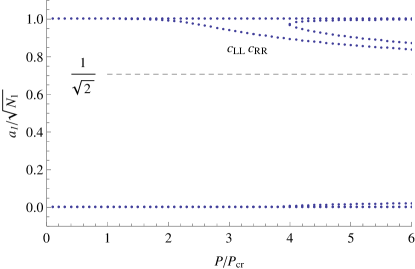
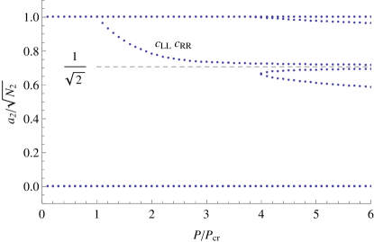
Figure 3: (Color online) Coefficients $a_{1}/\sqrt{N_{1}}$ and $a_{2}/\sqrt{N_{2}}$ defining the molecular states $\psi_{1},\psi_{2}$ of a two-species mixture as a function of $P/P_{\mathrm{cr}}$. The coefficients have been obtained by solving numerically Eq. (19) in the case of a $\mathrm{NH}_{3}$–$\mathrm{ND}_{3}$ mixture ($\mathrm{ND}_{3}$ is species $i=2$) with $x_{2}=0.1$ at temperature $T=300~{}\mathrm{K}$. The coefficients bifurcating at $P=P_{\mathrm{cr}}$ and tending for $P\gg P_{\mathrm{cr}}$ to $1/\sqrt{2}$ (dashed line) describe two degenerate molecular states, named $c_{LL}$ and $c_{RR}$, with molecules of both species in a chiral configuration of type $L$ or $R$. Notice further bifurcations appearing at $P\simeq 4P_{\mathrm{cr}}$, they correspond to stationary states of higher energy.

In conclusion, similarly to the case of a single chiral gas, it exists a critical pressure $P_{\mathrm{cr}}$ and a quantum phase transition taking place at $P=P_{\mathrm{cr}}$. For $0<P<P_{\mathrm{cr}}$, the lowest-energy stationary state of the mixture is the delocalized $d_{++}$ configuration given by Eq. (20). At $P=P_{\mathrm{cr}}$ a bifurcation occurs and two new energy-degenerate stationary states appear (see Fig. 3 for an example). We call them $c_{LL}$ and $c_{RR}$ because they correspond to molecules of both species in a chiral configuration of type $L$ or $R$ (see Table 2), achieving a complete localization for $P\gg P_{\mathrm{cr}}$. The value of $P_{\mathrm{cr}}$ is given by Eq. (23). This formula says that the inverse critical pressure of the mixture is the fraction-weighted average of the inverse critical pressures of its components,

$$\frac{1}{P_{\mathrm{cr}}}=\sum_{i=1}^{2}x_{i}\frac{1}{P^{(i)}_{\mathrm{cr}}},\qquad P^{(i)}_{\mathrm{cr}}=\frac{\Delta E_{i}}{2\gamma_{ii}}.$$ (25)

The difference between the lowest-energy stationary solutions of the two phases, namely, $d_{++}$ and $c_{LL},c_{RR}$, can be entirely encoded in the parameters

$$q_{i}=\left\{\begin{array}[]{ll}1,&\qquad P<P_{\mathrm{cr}},\\ 2a_{i}^{2}/N_{i}-1,&\qquad P>P_{\mathrm{cr}},\end{array}\right.,\qquad i=1,2,$$

(see Table 2). An example of the behavior of $q_{1}$ and $q_{2}$ as a function of the pressure is shown in Fig. 4. Each parameter $q_{i}$ vanishes for $P\to\infty$. More precisely, by using Eq. (19) it is simple to show that at the leading order for $P$ large one has

$$q_{i}=\frac{\gamma_{ii}}{\sum_{j=1}^{2}\gamma_{ij}x_{j}}~{}\frac{P_{\mathrm{cr}}^{(i)}}{P},$$ (26)

where $P_{\mathrm{cr}}^{(i)}$ is the critical pressure of the $i$th species as given by Eq. (25).

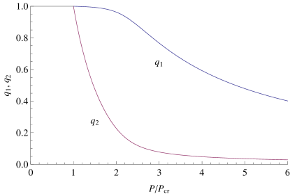
Figure 4: (Color online) Parameters $q_{1},q_{2}$ encoding the difference between the delocalized symmetric state $d_{++}$ and the chiral states $c_{LL}$ and $c_{RR}$ of Table 2 evaluated numerically for the same mixture of Fig. 3.

V.2 Excitation energies: Normal modes, inversion frequencies

As in the case of a single chiral species, we can determine the excitation energies from the ground state of a binary mixture by evaluating the linear response to an external time-dependent perturbation representing an electro-magnetic radiation. In detail, we modify the Hamiltonians (14) by adding for each species $i=1,2$ a perturbation of the form $\mu_{i}F(t)\sigma_{i}^{z}$ with the field $F(t)=F\cos(\omega t)$ sufficiently small so that effects of order $O(F^{2})$ are negligible. The perturbation induces a modified time evolution of the unperturbed ground state of the system which we evaluate as follows.

For $P<P_{\mathrm{cr}}$, the ground state of the mixture at zero external field is the symmetric delocalized state $d_{++}$ defined by the coefficients $(a_{1},b_{1},a_{2},b_{2})$ given by Eq. (20). For $P>P_{\mathrm{cr}}$, the unperturbed mixture has two lowest-energy degenerate stationary states, namely, the states $c_{LL}$ and $c_{RR}$, defined by the two sets of coefficients $(a_{1},b_{1},a_{2},b_{2})$ and $(a_{1},-b_{1},a_{2},-b_{2})$ given in Table 2 in terms of the parameters $q_{1},q_{2}$. For a racemic mixture, which is usually the case of concern, we may assume that the unperturbed ground state of species $i=1,2$ in the localized phase is represented by the stationary density matrix obtained by summing with equal weights the pure chiral states of types $L$ and $R$

$$\varrho_{i}^{(0)} =\frac{1}{2}\left(\begin{array}[]{c}a_{i}\\ b_{i}\end{array}\right)\left(\begin{array}[]{cc}a_{i}&b_{i}\end{array}\right)+\frac{1}{2}\left(\begin{array}[]{c}a_{i}\\ -b_{i}\end{array}\right)\left(\begin{array}[]{cc}a_{i}&-b_{i}\end{array}\right)$$ (33)

$$=\frac{N_{i}}{2}\left(\mathbb{1}_{i}+q_{i}\sigma_{i}^{x}\right).$$ (34)

Since for $P<P_{\mathrm{cr}}$ we have $q_{1}=q_{2}=1$, Eq. (34) represents the ground-state density matrix of the species $i=1,2$ also in the delocalized phase. In conclusion, we can analyze simultaneously both phases $P\gtrless P_{\mathrm{cr}}$ assuming that the unperturbed lowest-energy stationary state is given by the density matrices $\varrho_{1}^{(0)},\varrho_{2}^{(0)}$ of Eq. (34).

Under the effect of the perturbation, the time evolution of the density matrices of the two species is governed by the equations

$$i\hbar\frac{\mathrm{d}}{\mathrm{d}{t}}\varrho_{1}(t) =[h_{1}(\varrho_{1}(t),\varrho_{2}(t))+\mu_{1}F(t)\sigma_{1}^{z},\varrho_{1}(t)],$$ (35a)

$$i\hbar\frac{\mathrm{d}}{\mathrm{d}{t}}\varrho_{2}(t) =[h_{2}(\varrho_{1}(t),\varrho_{2}(t))+\mu_{2}F(t)\sigma_{2}^{z},\varrho_{2}(t)],$$ (35b)

where the mean-field Hamiltonians $h_{i}(\varrho_{1},\varrho_{2})$, $i=1,2$, are the same as Eq. (14) only rewritten in terms of the density matrices $\varrho_{1},\varrho_{2}$

$$h_{i}(\varrho_{1},\varrho_{2})=-\frac{\Delta E_{i}}{2}\sigma_{i}^{x}-\sum_{j=1}^{2}g_{ij}\mathop{\mathrm{tr}}\limits\left(\sigma_{j}^{z}\varrho_{j}\right)\sigma_{i}^{z}.$$ (36)

The density matrix of the $i$th species at time $t$ is written as

$$\varrho_{i}(t)=\varrho_{i}^{(0)}+x_{i}(t)\sigma_{i}^{x}+y_{i}(t)\sigma_{i}^{y}+z_{i}(t)\sigma_{i}^{z}.$$ (37)

Neglecting second order terms in the perturbation, the Bloch vector $(x_{i}(t),y_{i}(t),z_{i}(t))$ is determined by the system of differential equations

$$\begin{array}[]{l}\hbar x^{\prime}_{i}(t)=0\\ \hbar y^{\prime}_{i}(t)=\Delta E_{i}z_{i}(t)-\sum_{j=1}^{2}2N_{i}q_{i}g_{ij}z_{j}(t)+N_{i}q_{i}\mu_{i}F(t)\\ \hbar z^{\prime}_{i}(t)=-\Delta E_{i}y_{i}(t)\end{array},$$

obtained by plugging the definition (37) into Eq. (35).

We are interested in evaluating the electric dipole moments of each species $i=1,2$, namely,

$$p_{i}(t)=\mu_{i}\mathop{\mathrm{tr}}\limits\left(\sigma_{i}^{z}\varrho_{i}(t)\right)=2\mu_{i}z_{i}(t).$$

From the differential equations for the Bloch vector, we find that the Fourier transforms $\tilde{p}_{1}(\omega),\tilde{p}_{2}(\omega)$ are given by the system of algebraic equations

$$\left(\hbar^{2}\omega^{2}-\Delta E_{i}^{2}\right)\tilde{p}_{i}(\omega)+\sum_{j=1}^{2}2N_{i}q_{i}\Delta E_{i}g_{ij}\tilde{p}_{j}(\omega)$$

$$\qquad=2\mu_{i}^{2}N_{i}q_{i}\Delta E_{i}\tilde{F}(\omega),\qquad i=1,2,$$ (38)

where $\tilde{F}(\omega)$ is the Fourier transform of the applied field. The frequency-dependent electric susceptibility of the $i$th species is finally evaluated as the ratio between the Fourier transform of the polarization density of that species and the Fourier transform of the applied field,

$$\chi_{i}(\omega)=\frac{\tilde{p}_{i}(\omega)/(N/\rho)}{\varepsilon_{0}\tilde{F}(\omega)},$$

where $N/\rho$ is the volume occupied by the mixture and $\varepsilon_{0}$ the vacuum dielectric constant note.units . As usual, the density of the mixture at pressure $P$ and temperature $T$ is assumed to be $\rho=P/k_{B}T$. By determining $\tilde{p}_{1}(\omega)$ and $\tilde{p}_{2}(\omega)$ from Eq. (38), we find that the susceptibility of the mixture, $\chi=\chi_{1}+\chi_{2}$, is given by

$$\chi(\omega)= \frac{\rho}{\varepsilon_{0}}\frac{C(\omega)}{D(\omega)},$$ (39)

where

$$C(\omega)= \ \xi_{1}\mu_{1}^{2}\left[\hbar^{2}\omega^{2}-\Delta E_{2}^{2}+\xi_{2}\left(\gamma_{22}-\gamma_{12}\right)P\right]$$

$$+\xi_{2}\mu_{2}^{2}\left[\hbar^{2}\omega^{2}-\Delta E_{1}^{2}+\xi_{1}\left(\gamma_{11}-\gamma_{21}\right)P\right],$$ (40)

$$D(\omega)= \left(\hbar^{2}\omega^{2}-\Delta E_{1}^{2}+\xi_{1}\gamma_{11}P\right)$$

$$\times\left(\hbar^{2}\omega^{2}-\Delta E_{2}^{2}+\xi_{2}\gamma_{22}P\right)-\xi_{1}\xi_{2}\gamma_{12}\gamma_{21}P^{2},$$ (41)

$$\xi_{i}= \ 2x_{i}q_{i}\Delta E_{i},\qquad i=1,2.$$ (42)

The poles of the linear-response function (39) provide the excitation energies from the ground state predicted by our mean-field model Blaizot-Ripka . It is worth to explore first two limit cases.

For noninteracting molecules, namely, $\gamma_{ij}=0$, $i,j=1,2$, we have

$$\chi(\omega)=\frac{\rho}{\varepsilon_{0}}\left(\frac{\xi_{1}\mu_{1}^{2}}{\hbar^{2}\omega^{2}-\Delta E_{1}^{2}}+\frac{\xi_{2}\mu_{2}^{2}}{\hbar^{2}\omega^{2}-\Delta E_{2}^{2}}\right).$$

As expected, the response to an electromagnetic radiation incident on the mixture would, in this case, provide excitation energies $\Delta E_{1}$ and $\Delta E_{2}$ corresponding to the inversion of isolated molecules of species 1 and 2.

For a gas with just one chiral species, let us say $x_{2}=0$, Eq. (39) reduces to

$$\chi(\omega)=\frac{\rho\mu_{1}^{2}}{\varepsilon_{0}}\frac{2q_{1}\Delta E_{1}}{\hbar^{2}\omega^{2}-\left(\Delta E_{1}^{2}-2q_{1}\Delta E_{1}\gamma_{11}P\right)}.$$

In this case we also have nota.gaspuro $q_{1}=1$ for $P<P_{\mathrm{cr}}$ and $q_{1}=\Delta E_{1}/(2G_{11})$ for $P>P_{\mathrm{cr}}$, where $G_{11}=\gamma_{11}P$, so that we recover the result of Eq. (56). The same conclusion is obtained if we consider a single chiral gas as the mixture of two identical species with arbitrary fractions $x_{1}$ and $x_{2}$ such that $x_{1}+x_{2}=1$.

For a general mixture, no partial cancellation of zeros between numerator and denominator of $\chi(\omega)$ takes place as in the above two limit cases. The poles of the electric susceptibility coincide with the zeros of $D(\omega)$. By using the property $\gamma_{11}\gamma_{22}-\gamma_{12}\gamma_{21}=0$, we find that the bi-quadratic equation $D(\omega)=0$ has solutions with modulus $\overline{\omega}_{\pm}$ given by

$$2\hbar^{2}\overline{\omega}_{\pm}^{2}= A_{12}\pm\sqrt{{A_{12}}^{2}-4B_{12}},$$ (43)

where

$$A_{12} =\Delta E_{1}^{2}+\Delta E_{2}^{2}-(\xi_{1}\gamma_{11}+\xi_{2}\gamma_{22})P,$$

$$B_{12} =\Delta E_{1}^{2}\Delta E_{2}^{2}-(\xi_{1}\gamma_{11}\Delta E_{2}^{2}+\xi_{2}\gamma_{22}\Delta E_{1}^{2})P.$$

Clearly, the excitation energies of the mixture $\hbar\overline{\omega}_{\pm}$ are functions of the pressure.

At $P=0$, the normal modes represent the inversion of isolated molecules of species 1 or 2, namely,

$$\hbar\overline{\omega}_{\pm}(0)=\Delta E_{i_{\pm}},$$

where $i_{+}=1$ and $i_{-}=2$ if $\Delta E_{1}>\Delta E_{2}$ and $i_{+}=2$ and $i_{-}=1$ if $\Delta E_{2}>\Delta E_{1}$.

In the delocalized phase $0<P<P_{\mathrm{cr}}$, we have

$$B_{12}(P)=\Delta E_{1}^{2}\Delta E_{2}^{2}\left(1-P/P_{\mathrm{cr}}\right),$$

in virtue of the fact that $q_{1}=q_{2}=1$. For the same reason we also have that $\xi_{1}$ and $\xi_{2}$ are constant in this phase so that $A_{12}(P)$ decreases linearly with $P$. As a result, we find that $\hbar\overline{\omega}_{\pm}(P)$ decrease from their $P=0$ value according to

$$\hbar\overline{\omega}_{\pm}(P)\simeq\Delta E_{i_{\pm}}\sqrt{1-\frac{P}{P_{\mathrm{cr}}^{(i_{\pm})}}}.$$

These approximated relations, which are merely the inversion frequency laws for the pure species [see Eq. (58)], are valid for $P$ small. The larger is the fraction of the species $i_{\pm}$, the wider is the range of $P$ where the approximation is adequate.

At $P=P_{\mathrm{cr}}$, we have $B_{12}(P_{\mathrm{cr}})=0$ and, according to Eq. (43), the energy $\hbar\overline{\omega}_{-}$ vanishes with an infinite slope. The energy of the other mode attains the finite value $\hbar\overline{\omega}_{+}=\sqrt{A_{12}(P_{\mathrm{cr}})}$.

In the localized phase $P>P_{\mathrm{cr}}$, where $q_{i}=2a_{i}^{2}/N_{i}-1$, $i=1,2$, with $a_{1}^{2}$ and $a_{2}^{2}$ satisfying Eq. (22), we have $B_{12}(P)=0$ for any value of $P$. It follows that $\hbar\overline{\omega}_{-}=0$ throughout this phase. The energy of the other mode persists in decreasing and for $P\gg P_{\mathrm{cr}}$ approaches the asymptotic value

$$\hbar\overline{\omega}_{+}^{\mathrm{as}}=\sqrt{\frac{\Delta E_{1}^{2}\gamma_{12}x_{2}}{\gamma_{11}x_{1}+\gamma_{12}x_{2}}+\frac{\Delta E_{2}^{2}\gamma_{21}x_{1}}{\gamma_{22}x_{2}+\gamma_{21}x_{1}}}.$$ (44)

This value corresponds to $\sqrt{A_{12}}$ evaluated with the leading order expressions of $q_{1},q_{2}$ as in Eq. (26).

In Figs. 5 and 6 we show the excitation energies $\hbar\overline{\omega}_{\pm}$ calculated for a $\mathrm{NH}_{3}$–$\mathrm{ND}_{3}$ mixture with 10% and 0.01% deuterated ammonia fraction, respectively.

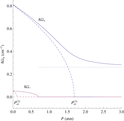
Figure 5: (Color online) Energies $\hbar\overline{\omega}_{\pm}$ of the excitation normal modes as a function of pressure $P$ in the case of a $\mathrm{NH}_{3}$–$\mathrm{ND}_{3}$ mixture ($\mathrm{ND}_{3}$ is species $i=2$) with $x_{2}=0.1$ at $T=300~{}\mathrm{K}$. The horizontal dotted line is the asymptotic value $\hbar\overline{\omega}_{+}^{\mathrm{as}}$. The dashed lines which vanish at $P_{\mathrm{cr}}^{(1)}=1.69~{}\mathrm{atm}$ and $P_{\mathrm{cr}}^{(2)}=0.11~{}\mathrm{atm}$ correspond to the inversion frequencies of pure species. The critical pressure of the mixture, point where $\hbar\overline{\omega}_{-}$ vanishes, is $P_{\mathrm{cr}}=0.70~{}\mathrm{atm}$. Energy is measured in $\textrm{cm}^{-1}$.

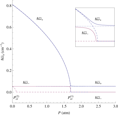
Figure 6: (Color online) As in Fig. 5 for $x_{2}=0.0001$. For such small value of $x_{2}$ the critical pressure of the mixture is $P_{\mathrm{cr}}\simeq P_{\mathrm{cr}}^{(1)}$ and we have $\hbar\overline{\omega}_{+}^{\mathrm{as}}\simeq\Delta E_{i_{-}}$. Inset is a zoomed in view of the region $P\simeq P_{\mathrm{cr}}$.

V.3 Consistency of the model: Absorption coefficient

We have already discussed the consistency of our model by considering two limiting cases in which it must recover the single gas case. In fact, we have observed that the susceptibility of a binary mixture reduces to that of a single chiral gas in the limit of fraction of one species tending to zero or in the limit in which the parameters defining the two species become equal. Here, we study in deeper details this limiting behavior by taking into account the absorption coefficient associated with the evaluated susceptibility.

According to the Beer-Lambert law, the intensity of a monochromatic radiation of angular frequency $\omega$ propagating for a length $\ell$ into the mixture is decreased by a factor $e^{-\kappa(\omega)\ell}$ due to the excitation of the normal modes. Neglecting deexcitation from these modes, i.e., spontaneous and stimulated reemission of radiation, the absorption coefficient is

$$\kappa(\omega)=\frac{\omega}{c}\mathop{\rm Im}\chi(\omega),$$ (45)

with $c$ speed of light and $\chi(\omega)$ as in Eq. (39). The imaginary part of susceptibility is evaluated with the prescription $\omega\to\omega-i\eta$ where $\eta\to 0^{+}$. The result is

$$\kappa(\omega)= I_{+}\left[\delta(\hbar\omega-\hbar\overline{\omega}_{+})+\delta(\hbar\omega+\hbar\overline{\omega}_{+})\right]$$ (46)

$$+I_{-}\left[\delta(\hbar\omega-\hbar\overline{\omega}_{-})+\delta(\hbar\omega+\hbar\overline{\omega}_{-})\right],$$

where the intensities $I_{\pm}$ are

$$I_{\pm}=\frac{\pi\rho}{2\varepsilon_{0}c\hbar}~{}\frac{C(\overline{\omega}_{\pm})}{\hbar^{2}\overline{\omega}_{\pm}^{2}-\hbar^{2}\overline{\omega}_{\mp}^{2}},$$ (47)

with $C(\omega)$ given by Eq. (40). These intensities depend on the pressure and for $P\to 0$ at the leading order they are

$$I_{\pm}(P)=x_{i_{\pm}}\frac{\pi\Delta E_{i_{\pm}}\mu_{i_{\pm}}^{2}}{\varepsilon_{0}c\hbar k_{B}T}P.$$ (48)

We have assumed, as usual, $\rho=P/(k_{B}T)$ and used the property $\hbar\overline{\omega}_{\pm}\to\Delta E_{i_{\pm}}$ for $P\to 0$. Thus, when the density vanishes and the inter-molecular interactions can be neglected, the absorption coefficient of the mixture is the sum of the absorption coefficients of the two isolated species weighted by the corresponding fractions.

Note that for non-interacting molecules, i.e., $\gamma_{ij}=0$, $i,j=1,2$, the intensities $I_{\pm}$ are as in Eq. (48), i.e., the absorption coefficient grows indefinitely with the pressure. On the other hand, for interacting molecules we obtain that for $P\to\infty$ the absorption coefficient approaches a constant value with asymptotic intensities

$$I_{+}^{\textrm{as}}= \ x_{1}\frac{\pi\Delta E_{1}\mu_{1}^{2}}{\varepsilon_{0}c\hbar k_{B}T}P_{\mathrm{cr}}^{(1)}\frac{\gamma_{11}}{\gamma_{11}x_{1}+\gamma_{12}x_{2}}\left[1-\left(\frac{\Delta E_{2}}{\hbar\overline{\omega}_{+}^{\mathrm{as}}}\right)^{2}\right]$$

$$+x_{2}\frac{\pi\Delta E_{2}\mu_{2}^{2}}{\varepsilon_{0}c\hbar k_{B}T}P_{\mathrm{cr}}^{(2)}\frac{\gamma_{22}}{\gamma_{22}x_{2}+\gamma_{21}x_{1}}\left[1-\left(\frac{\Delta E_{1}}{\hbar\overline{\omega}_{+}^{\mathrm{as}}}\right)^{2}\right],$$

$$I_{-}^{\textrm{as}}= \ x_{1}\frac{\pi\Delta E_{1}\mu_{1}^{2}}{\varepsilon_{0}c\hbar k_{B}T}P_{\mathrm{cr}}^{(1)}\frac{\gamma_{11}}{\gamma_{11}x_{1}+\gamma_{12}x_{2}}\left(\frac{\Delta E_{2}}{\hbar\overline{\omega}_{+}^{\mathrm{as}}}\right)^{2}$$

$$+x_{2}\frac{\pi\Delta E_{2}\mu_{2}^{2}}{\varepsilon_{0}c\hbar k_{B}T}P_{\mathrm{cr}}^{(2)}\frac{\gamma_{22}}{\gamma_{22}x_{2}+\gamma_{21}x_{1}}\left(\frac{\Delta E_{1}}{\hbar\overline{\omega}_{+}^{\mathrm{as}}}\right)^{2}.$$

To understand the limit of the absorption coefficient for, e.g., $x_{2}\to 0$, observe that when the fraction of species 2 vanishes we have $P_{\mathrm{cr}}\to P_{\mathrm{cr}}^{(1)}$ and the limit frequencies are

$$\hbar\overline{\omega}_{+}\to\left\{\begin{array}[]{ll}\Delta E_{1}\sqrt{1-P/P_{\mathrm{cr}}^{(1)}},&\qquad P<P_{\mathrm{cr}}^{(1)}\\ \Delta E_{2},&\qquad P>P_{\mathrm{cr}}^{(1)}\end{array}\right.,$$

$$\hbar\overline{\omega}_{-}\to\left\{\begin{array}[]{ll}\Delta E_{2},&\qquad P<P_{\mathrm{cr}}^{(1)}\\ 0,&\qquad P>P_{\mathrm{cr}}^{(1)}\end{array}\right.,$$

if $\Delta E_{1}>\Delta E_{2}$, whereas for $\Delta E_{2}>\Delta E_{1}$ we have

$$\hbar\overline{\omega}_{+}\to\Delta E_{2},$$

$$\hbar\overline{\omega}_{-}\to\left\{\begin{array}[]{ll}\Delta E_{1}\sqrt{1-P/P_{\mathrm{cr}}^{(1)}},&\qquad P<P_{\mathrm{cr}}^{(1)}\\ 0,&\qquad P>P_{\mathrm{cr}}^{(1)}\end{array}\right..$$

From Eq. (47) it follows that

$$I_{+}\to\frac{\pi\Delta E_{1}\mu_{1}^{2}}{\varepsilon_{0}c\hbar k_{B}T}\left\{\begin{array}[]{ll}P,&\qquad P<P_{\mathrm{cr}}^{(1)}\\ 0,&\qquad P>P_{\mathrm{cr}}^{(1)}\end{array}\right.,$$

$$I_{-}\to\frac{\pi\Delta E_{1}\mu_{1}^{2}}{\varepsilon_{0}c\hbar k_{B}T}\left\{\begin{array}[]{ll}0,&\qquad P<P_{\mathrm{cr}}^{(1)}\\ P_{\mathrm{cr}}^{(1)},&\qquad P>P_{\mathrm{cr}}^{(1)}\end{array}\right.,$$

if $\Delta E_{1}>\Delta E_{2}$, whereas for $\Delta E_{2}>\Delta E_{1}$ we have

$$I_{+}\to 0,$$

$$I_{-}\to\frac{\pi\Delta E_{1}\mu_{1}^{2}}{\varepsilon_{0}c\hbar k_{B}T}\left\{\begin{array}[]{ll}P&\qquad P<P_{\mathrm{cr}}^{(1)}\\ P_{\mathrm{cr}}^{(1)}&\qquad P>P_{\mathrm{cr}}^{(1)}\end{array}\right..$$

In both cases, we recover the intensity of the pure chiral gas 1, increasing linearly with $P$ in the delocalized phase and locked at a constant value in the localized one.

In the limit $x_{1}\to 0$ one has similar formulas which can be obtained from the above ones by exchanging the indices $1\leftrightarrow 2$.

An example of the behavior of the intensities $I_{\pm}$ as a function of pressure $P$ is illustrated in Figs. 7 and 8 for the same $\mathrm{NH}_{3}$–$\mathrm{ND}_{3}$ mixtures considered in Figs. 5 and 6, respectively. In this case we have $\Delta E_{1}>\Delta E_{2}$ and the fraction $x_{2}$ decreases form $0.1$, Figs. 5 and 7, to $0.0001$, Figs. 6 and 8. The dominant intensity, $I_{+}$ or $I_{-}$, is mainly due to the more abundant species $i=1$.

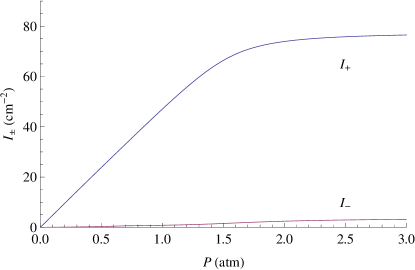
Figure 7: (Color online) Intensities $I_{\pm}$ of the absorption coefficient as a function of pressure $P$ for the mixture of Fig. 5. Energy is measured in $\textrm{cm}^{-1}$ and intensities, which have dimensions energy divided by length, are given in $\textrm{cm}^{-2}$.

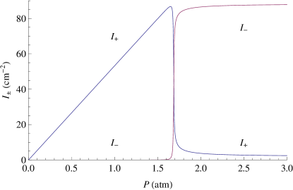
Figure 8: (Color online) As in Fig. 7 for the mixture of Fig. 6.

We now discuss the limit in which $\Delta E_{1},\Delta E_{2}\to\Delta E$, $\mu_{1},\mu_{2}\to\mu$ and $\gamma_{i,j}\to\gamma$, $i,j=1,2$, whereas $x_{1}$ and $x_{2}$ are arbitrary with $x_{1}+x_{2}=1$. In this case we have

$$\hbar\overline{\omega}_{+}\to\Delta E,$$

$$\hbar\overline{\omega}_{-}\to\left\{\begin{array}[]{ll}\Delta E\sqrt{1-P/P_{\mathrm{cr}}},&\qquad P<P_{\mathrm{cr}}\\ 0,&\qquad P>P_{\mathrm{cr}}\end{array}\right.,$$

where $P_{\mathrm{cr}}=\Delta E/(2\gamma)$. It is simple to verify that

$$I_{+}\to 0,$$

$$I_{-}\to\frac{\pi\Delta E\mu^{2}}{\varepsilon_{0}c\hbar k_{B}T}\left\{\begin{array}[]{ll}P,&\qquad P<P_{\mathrm{cr}}\\ P_{\mathrm{cr}},&\qquad P>P_{\mathrm{cr}}\end{array}\right.,$$

which is again the result for a single species characterized by the parameters $\Delta E$, $\mu$ and $\gamma$.

Due to line broadening, which in the microwave region of interest for a $\mathrm{NH}_{3}$–$\mathrm{ND}_{3}$ mixture is mostly due to molecular scattering, the absorption coefficient discussed above can not be directly compared with that measured in an experiment. However, a test of the excitation energies (43) could be done in an indirect way as in Bleaney-Loubster.1948 ; Bleaney-Loubster.1950 ; Birnbaum-Maryott.1953b . In these experiments the spectrum of the absorption coefficient measured for $\mathrm{NH}_{3}$ or $\mathrm{ND}_{3}$ at different pressures was fitted by a Van Vleck–Weisskopf formula VVW in which the center line frequency is considered a fitting parameter. The results of the fit are in excellent agreement with the predictions of our model for a single chiral gas, see jptprl or Appendix C. In the case of a $\mathrm{NH}_{3}$–$\mathrm{ND}_{3}$ mixture the situation is not different. If our model is correct, with a 10% $\mathrm{ND}_{3}$ fraction one should measure an absorption spectrum, mainly due to the $\hbar\overline{\omega}_{+}$ excitation mode, see Fig. 7, centered at a frequency which at high pressures approaches the value of $0.26~{}\textrm{cm}^{-1}$, see Fig. 5. This is a striking difference with respect to the case of a pure $\mathrm{NH}_{3}$ gas in which the center line frequency of the absorption spectrum vanishes for $P>1.69~{}\textrm{atm}$. Also the behavior of $\hbar\overline{\omega}_{-}(P)$ is rather different from the inversion frequency of pure $\mathrm{ND}_{3}$. In fact, the two frequencies vanish at $0.70~{}\textrm{atm}$ and $0.11~{}\textrm{atm}$, respectively. However, this effect should be more difficult to measure as the intensity $I_{-}$ is much lower than $I_{+}$, see Fig. 7.

VI Final remarks

Our approach to the existence of chiral molecules is based on ideas of equilibrium statistical mechanics. One may be surprised by the presence of a quantum phase transition at room temperatures. We emphasize that the transition takes place only in the inversion degrees of freedom. The dynamics of these degrees of freedom is affected by temperature only through the values of the coupling constants. A derivation of our approach from first principles is an open question. As we have discussed, in the case of a pure gas of ammonia or deuterated ammonia, our model compares very well with experimental results.

The problem of existence of chiral molecules has been approached also from a dynamical point of view TH ; BB ; CGG in terms of the quantum linear evolution with a Lindblad term. The question asked by these authors is how long a molecule in a chiral localized state remains in this state considering the interaction with the environment. This question had already been posed by Hund Hund without, however, any quantitative estimate. In Refs. TH ; BB , a calculation ab initio is discussed exploiting a mechanism whose basic idea goes back to Simonius ; Harris-Stodolsky : through repeated scatterings in a host gas, a molecule is blocked in a localized state. A detailed analysis of the decoherence of a two-state tunneling molecule due to collisions with a host gas is given in CGG in terms of a succession of quantum states of the molecule satisfying the conditions for a consistent family of histories.

Effective nonlinearities, closer to our interpretation, were considered in a dynamical context by Silbey-Harris and qualitatively connected to the disappearance of the inversion line. However, no quantitative estimate was attempted. In gsjpa dissipative effects are included in a nonlinear time-dependent model obtaining qualitative conclusions similar to jptprl . What is missing is a theory of the parameters of the model.

An important test of the present theory is to verify the shift of the critical pressure depending on the percentage of the two species in a binary mixture, e.g., $\mathrm{NH}_{3}$–$\mathrm{ND}_{3}$. As we have shown an addition of 10% of $\mathrm{ND}_{3}$ is sufficient to halve the critical pressure of pure $\mathrm{NH}_{3}$ and to appreciably change the dependence on pressure of the inversion frequencies of both species.

The interpretation of the experimental data Bleaney-Loubster.1948 ; Bleaney-Loubster.1950 ; Birnbaum-Maryott.1953b is based on the Van Vleck–Weisskopf formula. The inversion line measured at sufficiently high pressures consists actually of a band of lines close to each other arising from different angular momentum states. At low pressures these lines can be resolved Bleaney-Penrose.1947 . We may ask the question whether this case can be discussed in terms of a mixture of different pre-chiral gases corresponding to ammonia molecules in different angular momentum states and study the crossover to higher pressures.

Appendix A Stationary states of a chiral gas

The nonlinear eigenvalue problem associated with Eq. (2) and the normalization condition, namely,

$$h(\psi_{\lambda})\psi_{\lambda}=\lambda\psi_{\lambda},\qquad\langle\psi_{\lambda},\psi_{\lambda}\rangle=N,$$ (49)

where

$$h(\psi)=-\frac{\Delta E}{2}\sigma^{x}-\frac{G}{N}\langle\psi,\sigma^{z}\psi\rangle\sigma^{z},$$

has different solutions depending on the value of the ratio $G/\Delta E$. To see it, let us write

$$\psi_{\lambda}=a_{\lambda}\varphi_{+}+b_{\lambda}\varphi_{-}.$$

The coefficients $a_{\lambda}$ and $b_{\lambda}$ can be chosen real and are normalized to the number of molecules in the gas, $a_{\lambda}^{2}+b_{\lambda}^{2}=N$. By inserting this expression into Eq. (49), we find that $a_{\lambda},b_{\lambda}$ are the solutions of the equation

$$\Delta Ea_{\lambda}b_{\lambda}=\frac{G}{N}\left(a_{\lambda}^{2}-b_{\lambda}^{2}\right)2a_{\lambda}b_{\lambda}.$$ (50)

Once a solution of this system is found, the corresponding eigenvalue is given by

$$\lambda N=-\frac{\Delta E}{2}\left(a_{\lambda}^{2}-b_{\lambda}^{2}\right)-\frac{4G}{N}a_{\lambda}^{2}b_{\lambda}^{2}.$$

For any value of $G$, Eq. (50) always admits solutions such that $a_{\lambda}b_{\lambda}=0$. Up to an irrelevant sign, there are two different solutions which satisfy this condition and the normalization rule, namely, the delocalized eigenstates

$$\psi_{\lambda_{1}}=\sqrt{N}\varphi_{+},\qquad\lambda_{1}=-\Delta E/2,$$ (51)

$$\psi_{\lambda_{2}}=\sqrt{N}\varphi_{-},\qquad\lambda_{2}=+\Delta E/2.$$ (52)

If $G>\Delta E/2$, there appear two further solutions such that $a_{\lambda}b_{\lambda}\neq 0$, namely, the roots of

$$2a_{\lambda}^{2}/N-1=\Delta E/(2G).$$ (53)

The corresponding eigenstates are

$$\psi_{\lambda_{3}}=\sqrt{N}\left(\sqrt{\frac{1}{2}+\frac{\Delta E}{4G}}~{}\varphi_{+}+\sqrt{\frac{1}{2}-\frac{\Delta E}{4G}}~{}\varphi_{-}\right),$$

$$\lambda_{3}=-G,$$ (54)

$$\psi_{\lambda_{4}}=\sqrt{N}\left(\sqrt{\frac{1}{2}+\frac{\Delta E}{4G}}~{}\varphi_{+}-\sqrt{\frac{1}{2}-\frac{\Delta E}{4G}}~{}\varphi_{-}\right).$$

$$\lambda_{4}=-G,$$ (55)

We call these states chiral in the sense that $\psi_{\lambda_{3}}=\sigma^{x}\psi_{\lambda_{4}}$ and $\psi_{\lambda_{4}}=\sigma^{x}\psi_{\lambda_{3}}$. In the limit $G\gg\Delta E$, the eigenstates $\psi_{\lambda_{3}}$ and $\psi_{\lambda_{4}}$ approach the localized states $\sqrt{N}\varphi_{L}$ and $\sqrt{N}\varphi_{R}$, respectively.

The states $\psi_{\lambda}$ determined above, are the stationary solutions $\psi(t)=\exp(-i\lambda t/\hbar)\psi_{\lambda}$ of the time-dependent nonlinear Schrödinger equation

$$i\hbar\frac{\mathrm{d}}{\mathrm{d}t}\psi(t)=h(\psi)\psi(t)$$

and the eigenvalue $\lambda$ is the Lagrange multiplier fixing the conservation of the number of molecules. Associated with any solution $\psi(t)$ of this equation there is a conserved energy given by

$$\mathcal{E}(\psi)=-\frac{\Delta E}{2}\langle\psi,\sigma^{x}\psi\rangle-\frac{G}{2N}\langle\psi,\sigma^{z}\psi\rangle^{2}.$$

The value of this functional calculated at the stationary solutions (51)–(55), i.e.,

$$\mathcal{E}(\psi_{\lambda})=-\frac{\Delta E}{2}\left(a_{\lambda}^{2}-b_{\lambda}^{2}\right)-\frac{2G}{N}a_{\lambda}^{2}b_{\lambda}^{2},$$

provides the corresponding single-molecule energies $e_{i}=\mathcal{E}(\psi_{\lambda_{i}})/N$, $i=1,\dots,4$,

$$e_{1}=-\frac{\Delta E}{2}$$

$$e_{2}=+\frac{\Delta E}{2}$$

$$e_{3}=e_{4}=-\frac{\Delta E}{2}-\frac{1}{2G}\left(\frac{\Delta E}{2}-G\right)^{2}.$$

These energies are plotted in Fig. 9 as a function of $G$. The molecular state effectively assumed by the gas is that with the minimal energy, namely, the symmetric delocalized state $\psi_{\lambda_{1}}$ for $G<\Delta E/2$, or one of the two degenerate chiral states $\psi_{\lambda_{3}}$, $\psi_{\lambda_{4}}$ for $G>\Delta E/2$.

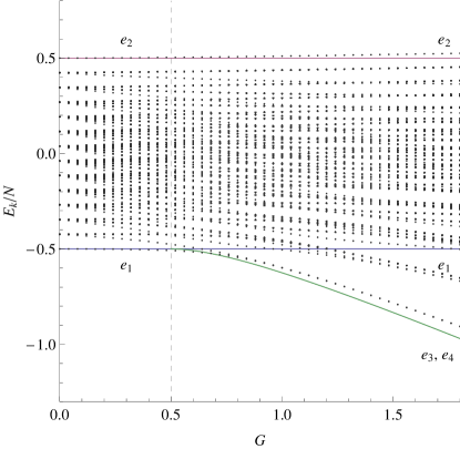
Figure 9: (Color online) Eigenvalues $E_{k}$, $k=1,\dots,2^{N}$, divided by $N$, of the $N$-body Hamiltonian of Eq. (1) with $\mathfrak{g}_{ij}=G/N$ and $N=13$ calculated numerically for different values of $G$ (dots). The solid lines are the single-molecule energies $e_{i}=\mathcal{E}(\psi_{\lambda_{i}})/N$ associated with the mean-field stationary states $\psi_{\lambda_{i}}$, $i=1,\dots,4$.

The above results imply a bifurcation of the mean-field ground state at a critical interaction strength $G_{\mathrm{cr}}=\Delta E/2$. According to Eq. (II), this transition can be obtained for a given molecular species by increasing the gas pressure above the critical value $P_{\mathrm{cr}}$ given by Eq. (4).

Appendix B Excitations from the ground state

It is interesting to compare the mean-field molecular states described in the previous section with the eigenstates of the $N$-body model (1). In the latter case, the Hamiltonian is represented by a $2^{N}\times 2^{N}$ matrix which, if $N$ is not too large, can be diagonalized numerically. For a meaningful comparison with the mean field we set $\mathfrak{g}_{ij}=G/N$. The eigenvalues obtained for $N=13$ are shown in Fig. 9 as a function of $G$. We see that there is a strict correspondence between the smallest and largest eigenvalues of (1) and the smallest and largest conserved energies associated with the mean-field eigenstates of (2). Assuming that the eigenstates of (1) are ordered according to their magnitude, $E_{1}<E_{2}<\dots,E_{2^{N}}$, we have

$$E_{1}\simeq\left\{\begin{array}[]{ll}\mathcal{E}(\psi_{\lambda_{1}}),&\quad G<\Delta E/2,\\ \mathcal{E}(\psi_{{\lambda_{3}},{\lambda_{4}}}),&\quad G>\Delta E/2,\end{array}\right.$$

$$E_{2^{N}}\simeq\mathcal{E}(\psi_{\lambda_{2}}).$$

By increasing the size $N$ of the system we find that the differences between the $N$-body and mean-field energies indicated above increase slower than $N$. Assuming that these differences are $o(N)$, in Fig. 9 we compare single-particle rescaled values, namely, $E_{k}/N$, $k=1,\dots,2^{N}$, and $e_{i}=\mathcal{E}(\psi_{\lambda_{i}})/N$, $i=1,\dots,4$. The results shown for $N=13$ already give an idea of what to expect for $N\to\infty$.

The diagonalization of the Hamiltonian (1) provides a full description of the excitation modes. The energy gap between the ground state and the first excited one, namely, $E_{2}-E_{1}$, is the inversion doubling, namely, the excitation of one quasi-molecule from the state $\varphi_{+}$ to the state $\varphi_{-}$. For $G=0$, the gap amounts exactly to $\Delta E$ and the excited level is $N$-fold degenerate. Due to the attractive dipole-dipole interaction, the value of the gap evaluated for $G>0$ is decreased with respect to the noninteracting case by an amount of the order of $G$. For $G$ large the ground state becomes two-fold degenerate and the gap vanishes. In Fig. 10 we show the value of $E_{2}-E_{1}$ evaluated as a function of $G$ for systems of increasing size $N$.

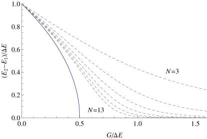
Figure 10: (Color online) Energy gap $E_{2}-E_{1}$ of the $N$-body Hamiltonian (1) with $\mathfrak{g}_{ij}=G/N$ and $N=3$, 5, 7, 9, 11, 13 (dashed lines from top to bottom) as a function of the ratio $G/\Delta E$. The solid line represents $\hbar\overline{\nu}/\Delta E$, where $\overline{\nu}$ is the inversion doubling frequency predicted by Eq. (57).

For any value of $N$ the gap vanishes smoothly at $G\gg\Delta E$, however, by increasing $N$ such smoothness becomes paler and paler. What is the behavior that we should expect in the $N\to\infty$ limit? As we will see in a moment, the mean-field indicates that $E_{2}-E_{1}$ sharply vanishes at $G=\Delta E/2$ thus suggesting that for $N\to\infty$ a phase transition takes place.

In general, the excitation energies from the ground state can be evaluated as the poles of the Fourier transform of the linear-response function Blaizot-Ripka . In jptprl , we have evaluated the linear response of the mean-field Hamiltonian (2) to a time-dependent perturbation which corresponds to an electro-magnetic radiation coupling with the electric dipole of the molecules. For a gas in the mean-field $\psi_{\lambda_{1}}$, the Fourier transform of the linear-response function is noteRCHI

$$\mathcal{R}(\omega)=\frac{2\Delta E}{(\hbar\omega)^{2}-(\Delta E^{2}-2G\Delta E)},$$ (56)

which has two simple poles at angular frequency $\pm\overline{\omega}$, $\overline{\omega}=\sqrt{\Delta E^{2}-2G\Delta E}/\hbar$. We conclude that, in the region $0\leq G<\Delta E/2$ where the gas is at equilibrium in the molecular state $\psi_{\lambda_{1}}$, the mean-field model predicts an inversion doubling frequency $\overline{\nu}=\overline{\omega}/(2\pi)$ given by

$$\overline{\nu}=\frac{\Delta E}{h}\sqrt{1-\frac{2G}{\Delta E}},$$ (57)

which vanishes at $G=\Delta E/2$. This behavior of $h\overline{\nu}$ is compatible with the $N\to\infty$ limit of the gap $E_{2}-E_{1}$ which can be envisaged from Fig. 10.

Appendix C Pressure dependence of $\mathrm{NH}_{3}$ and $\mathrm{ND}_{3}$ inversion lines: comparison with experiments

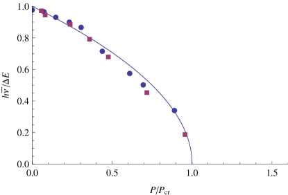
Figure 11: (Color online) Plot of the universal function of Eq. (58). Points are the experimental results for $\mathrm{NH}_{3}$ (circles) or $\mathrm{ND}_{3}$ (squares) available from Ref. Bleaney-Loubster.1948 ; Bleaney-Loubster.1950 and Birnbaum-Maryott.1953b , respectively. The experimental data have been scaled using the values of $\Delta E$ and $P_{\mathrm{cr}}$ from Table 1.

.

In jptprl , we have compared the mean-field theoretical prediction for the inversion frequency with the spectroscopic data available for ammonia Bleaney-Loubster.1948 ; Bleaney-Loubster.1950 and deuterated ammonia Birnbaum-Maryott.1953b . In these experiments, the central frequency of the inversion peak was measured at different pressures. The frequency is found to decrease by increasing $P$ and vanishes for pressures greater than a critical value. This behavior is very well accounted for by the mean-field prediction (57) for $\overline{\nu}$. In fact, an important feature of this equation is the statement that the ratio between the frequency $\overline{\nu}$ of a measured spectroscopic inversion line and the energy splitting $\Delta E$ of an isolated molecule,

$$\frac{h\overline{\nu}}{\Delta E}=\sqrt{1-\frac{P}{P_{\mathrm{cr}}}},$$ (58)

is a universal function of $P/P_{\mathrm{cr}}$ independent of the kind of chiral species considered. In Fig. 11, we show the values of $h\overline{\nu}/\Delta E$ measured at different pressures $P$ in the case of ammonia and deuterated ammonia. The superposition of the two sets of data plotted as a function of $P/P_{\mathrm{cr}}$ and the agreement with formula (58) is impressive.

Some comments are in order. The mean-field prediction (58) does not contain free parameters. The value of $P_{\mathrm{cr}}$ is evaluated from the electric dipole $\mu$ of the molecule, its collision diameter $d$ and inversion energy splitting $\Delta E$, and the temperature $T$ of the gas, see Eq. (4) and Table 1. We remark, however, that the experimental points shown in Fig. 11 are the result of an indirect measurement. More precisely, in experiments Bleaney-Loubster.1948 ; Bleaney-Loubster.1950 ; Birnbaum-Maryott.1953b the line shape of the absorption coefficient measured for $\mathrm{NH}_{3}$ and $\mathrm{ND}_{3}$ at different pressures $P$ is fitted by a Van Vleck–Weisskopf formula VVW in which $\overline{\nu}$ is a considered a fitting parameter.

References

- (1) F. Hund, Z. Phys. 43, 805 (1927).
- (2) P.W. Anderson, Phys. Rev. 75, 1450 (1949).
- (3) P. Claverie and G. Jona-Lasinio, Phys. Rev. A 33, 2245 (1986).
- (4) G. Jona-Lasinio and P. Claverie, Prog. Theor. Phys. Suppl. 86, 54 (1986).
- (5) A. S. Wightman, Il nuovo Cimento 110 B, 751 (1995).
- (6) V. Grecchi and A. Martinez, Comm. Math. Phys. 166, 533 (1995).
- (7) G. Jona-Lasinio, C. Presilla, and C. Toninelli, Phys. Rev. Lett. 88, 123001 (2002).
- (8) G. Jona-Lasinio, Prog. Theor. Phys. 124, 731 (2010).
- (9) B. Bleaney and J. H. Loubster, Nature 161, 522 (1948).
- (10) B. Bleaney and J. H. Loubster, Proc. Phys. Soc. (London) A63, 483 (1950).
- (11) G. Birnbaum and A. Maryott, Phys. Rev. 92, 270 (1953).
- (12) T. R. Hanley, P.G. Steffes, and B. M. Karpowicz, Icarus 202, 316 (2009).
- (13) W. H. Keesom, Physik. Z. 22, 129 (1921).
- (14) C. H. Townes and A. L. Schawlow, Microwave Spectroscopy (Mc Graw-Hill, New York, 1955).
- (15) CRC Handbook of Chemistry and Physics, edited by D. R. Lide (CRC Press, New York, 1995), 76th ed..
- (16) L. Onsager, J. Am. Chem. Soc. 58, 1486 (1936).
- (17) C. T. F. Böttcher, Theory of Electric Polarization (Elsevier, Amsterdam, 1973).
- (18) B. Linder and D. Hoernschemeyer, J. Chem. Phys. 46, 784 (1966).
- (19) F. Hynne and R. K. Bullough, J. Phys. A 5, 1272 (1972).
- (20) We use SI units. The expression of in the Gauss system of units is obtained by changing .
- (21) J. P. Blaizot and G. Ripka, Quantum Theory of Finite Systems (The MIT Press, Cambridge, MA, 1986).
- (22) For a single chiral gas in the localized phase we have , see Eq. (53).
- (23) J. H. Van Vleck and V. F. Weisskopf, Rev. Mod. Phys. 17, 227 (1945).
- (24) J. Trost and K. Hornberger, Phys. Rev. Lett. 103, 023202 (2009).
- (25) M. Bahrami and A. Bassi, Phys. Rev. A 84, 062115 (2011).
- (26) P. J. Coles, V. Gheorghiu, and R. B. Griffiths, Phys. Rev. A 86, 042111 (2012).
- (27) M. Simonius, Phys. Rev. Lett. 40, 980 (1978).
- (28) R. A. Harris and L. Stodolsky, Phys. Lett. B 78, 313 (1978); J. Chem. Phys. 74, 2145 (1981); Phys. Lett. B 116, 464 (1982); J. Chem. Phys. 78, 7330 (1983).
- (29) R. Silbey, R. A. Harris, J. Phys. Chem. 93, 7062 (1989).
- (30) V. Grecchi and A. Sacchetti, J. Phys. A 37, 3527 (2004).
- (31) B. Bleaney and R. P. Penrose, Proc. Roy. Soc. A189, 358 (1947).
- (32) The linear-response function coincides up to a constant, namely, , with the single-species limit of the susceptibility determined in Section V.2. Note that has been evaluated in jptprl only in the delocalized phase , while is given also in the localized phase.