Submm-bright X-ray absorbed QSOs at z$\sim$2: insights into the co-evolution of AGN and star-formation

Abstract

We have assembled a sample of 5 X-ray-absorbed and submm-luminous type 1 QSOs at $z\sim 2$ which are simultaneously growing their central black holes through accretion and forming stars copiously. We present here the analysis of their rest-frame UV to submm Spectral Energy Distributions (SEDs), including new Herschel data. Both AGN (direct and reprocessed) and Star Formation (SF) emission are needed to model their SEDs. From the SEDs and their UV-optical spectra we have estimated the masses of their black holes $M_{BH}\sim 10^{9}-10^{10}\,M_{\odot}$, their intrinsic AGN bolometric luminosities $L_{BOL}\sim(0.8-20)\times 10^{13}L_{\odot}$, Eddington ratios $L_{BOL}/L_{Edd}\sim 0.1-1.1$ and bolometric corrections $L_{BOL}/L_{X,2-10}\sim 30-500$. These values are common among optically and X-ray-selected type 1 QSOs (except for RX J1249), except for the bolometric corrections, which are higher. These objects show very high far-infrared luminosities $L_{FIR}\sim$ (2 - 8)$\times 10^{12}\,M_{\odot}$ and Star Formation Rates SFR$\sim 1000M_{\odot}/$y. From their $L_{FIR}$ and the shape of their FIR-submm emission we have estimated star-forming dust masses of $M_{DUST}\sim 10^{9}\,M_{\odot}$. We have found evidence of a tentative correlation between the gas column densities of the ionized absorbers detected in X-ray (N${}_{H_{ion}}$) and $SFR$. Our computed black hole masses are amongst the most massive known.

1 Introduction

In the last two decades, it has become clear that most local spheroidal galaxy components (elliptical galaxies and the bulges of spiral galaxies) contain a super massive black hole (SMBH) in their centres. The proportionality between black hole (BH) and spheroid mass suggests a direct link between the growth of the black hole as an Active Galactic Nucleus (AGN) and the stellar mass of the spheroid (e.g. Marconi et al. 2004, Kormendy & Ho 2013). Identifying the main mechanisms for formation and evolution of galaxies, and their interrelation to that of the growth of their central black holes is a major issue in Astrophysics and Cosmology.

In the last decade, deep surveys at submillimetre (submm) and millimetre (mm) wavelengths have identified a high-redshift population of massive dusty galaxies that are undergoing extreme starbursts. Since prodigious star formation (SF) is often obscured by dust, these galaxies are luminous in the mm though far-infrared (FIR) wavebands where the starlight absorbed by dust grains is re-emitted. Likewise, the hotter dust heated in the circumnuclear environment of an AGN will emit at mid-infrared (MIR) wavelengths. Therefore, submm and MIR observations can be combined to study activity in galaxies due to dust-obscured starbursts and AGN. The launch of the Herschel Space Observatory data (Pilbratt et al., 2010) allow obtaining more accurate and deeper measurements in the FIR, permitting better determinations of the luminosity due to SF ($L_{SF}$) and hence the SFR. In recent years there have been many studies in which the SFR was compared with the growth of the central BH (Rovilos et al. 2012, Page et al. 2012, Rosario et al. 2012, Lutz et al. 2008) with conflicting results about the relationship between AGN luminosity and $L_{SF}$ .

In this paper, we have studied a sample of X-ray-obscured QSOs, described by Page et al. (2004) and Stevens et al. (2005), and studied by Stevens et al. (2004); Stevens et al. (2010), Page et al. (2011) and Carrera et al. (2011) (20 unabsorbed objects), at z$\sim$1-3 when most of the SF and BH growth are occurring in the Universe. Stevens et al. (2005) found six detections at $>5\sigma$ significance at 850$\mu$m (SCUBA). These QSOs have strong submm emission, much higher than typically found in QSOs at similar redshifts and luminosities. However for one of them (RX J110431.75 + 355208.5) a synchrotron origin for the detected 850$\mu$m emission cannot be ruled out, so we have not followed up RX J110431.75 in this work, and our sample consists of the other five sources. They were specifically targeted with Herschel Space Observatory data OT 1 (PI: F.J. Carrera).

The ultraviolet (UV) and X-ray spectra of our QSOs show evidence for strong ionized winds which produce the X-ray obscuration (Page et al., 2011). Piecing all these clues together, we inferred that the host galaxies of these QSOs are undergoing strong SF, while the central SMBH are also growing through accretion. In principle the ionized winds are strong enough to quench the SF (Page et al., 2011) so, given that the QSOs have powerful submm emission, these objects are then caught at a special time, perhaps emerging from a strongly obscured accretion state in an evolutionary stage which might last about 10-15 per cent of the QSO lifetime (Hopkins et al., 2008), which tallies nicely with X-ray absorbed broad line AGN being about 15 per cent of the X-ray broad line population (e.g. Page, Mittaz, & Carrera 2000; Mateos et al. 2010; Corral et al. 2011; Scott et al. 2011; Scott, Stewart, & Mateos 2012). Alternatively, the ionized winds are de-coupled from the SF, but then why only X-ray-absorbed AGN are submm-luminous remains to be explained. Some geometrical effect might be invoked, but it is difficult to see how to reconcile the dramatically different scales at which both processes are expected to happen.

Here, we endeavour to get the physical properties of the central QSOs (luminosities, BH masses, Eddington ratios, etc.) and their host galaxies (SFR, $M_{DUST}$, $M_{GAS}$, etc.) and their mutual relationships (or lack thereof). In addition, we will try to fathom their place in AGN-host galaxy co-evolution models.

The paper is organized as follows. In Section 2, we present our sample and summarize the data used. In Section 3, we present the Spectral Energy Distributions (SEDs) of all our objects, explain how we have made fits to several representative templates and obtained results from them. Moreover, we calculate the Black Hole properties from UV-Optical spectra and we study the time scales of the evolution of the AGN and the host galaxy. In section 4, we discuss all results and compare them with those found in other samples. Finally, we summarize our findings in Section 5.

We have assumed throughout this paper a Hubble constant $H_{0}=70$ km/s/Mpc, and density parameters $\Omega_{\mathrm{m}}=0.3$ and $\Omega_{\Lambda}=0.7$.

2 Data

We present in Table 1 Herschel Space Observatory data for the fields around our QSOs (RX J0057, RX J0941, RX J1218, RX J1249, RX J1633). These data include two photometric bands (100$\mu$m and 160$\mu$m) from the PACS instrument (Poglitsch et al., 2010) and three photometric SPIRE bands (250$\mu$m, 350$\mu$m and 500$\mu$m); Griffin et al. (2010), see Table 2. The PACS observations were performed in two scan orientations (70ºand 110º) for each band and field. These images were combined using the standard pipeline of Herschel Interactive Processing Environment (HIPE v8 and v10). The SPIRE were undertaken in smallmap mode. We used directly Level 2 data obtained from the Herschel Archive and implemented a script to remove the background from the data (UKIRT Newsletter., 2010). We also present here new optical imaging data (R filter) from the William Herschel Telescope for RX J1249. The observations were taken on 20th May of 2010. The reduction and calibration were carried out using standard iraf procedures (see Carrera et al. 2011 for details).

In addition, part of the data used in this paper have been used or obtained in other studies: X-ray spectroscopic observations from XMM-Newton and optical-UV spectra from Page et al. (2001, 2011), Spitzer and SCUBA photometric data from Stevens et al. (2004); Stevens et al. (2010) and optical and infrared photometric data for RX J0941 from Carrera et al. (2011). Finally, we have also used public data from different catalogues (SDSS, 2MASS, SUPERCOSMOS, WISE, GALEX and OM-SUSS), see Table 2.

We have used Sloan PSF magnitudes, converting them to fluxes directly using $m_{AB}=-2.5\log(F_{\nu})-48.60$ with $f_{\nu_{0}}=3.63\times 10^{3}$Jy. For $u$ and $z$ we have converted previous to AB magnitude using :

$$u_{AB}=u_{SDSS}-0.04\\ z_{AB}=z_{SDSS}+0.02$$ (1)

For non-AB magnitudes we have used :

$$F_{\nu}=F_{\nu,0}\times 10^{-0.4m}$$ (2)

where $F_{\nu,0}$ are given in column 3 in Table 2 for each band.

A conservative 5 per cent error was added in quadrature to the Herschel (extracted from HIPE documentation), SDSS and SUPERCOSMOS (Hambly, Irwin, & MacGillivray, 2001) catalogued flux errors to account for the uncertainties in the zero-points. In addition, we have also added in quadrature a 2 per cent error for the 2MASS data (Cohen, Wheaton, & Megeath, 2003). Regarding data from WISE, we have added a 1.5 per cent uncertainty to the catalogued flux errors in all bands to account for the overall systematic uncertainty from the Vega spectrum in the flux zero-points. Additionally we have added a 10 per cent uncertaintyto the 12 µm and 22 µm fluxes (Wright et al., 2010) to account the existing discrepancy between the red and blue calibrators used for the conversion from magnitudes to Janskys.

Table 1: Summary of the Herschel observations on our fields.

Object	$RA$	$DEC$	z	OBSID PACS	Date Obs.	OBSID SPIRE	Date Obs.
RX J0057	$00:57:34.94$	$-27:28:28.0$	2.19	1342225345-6	2011-07-23	1342234705	2011-12-18
RX J0941	$09:41:44.61$	$+38:54:39.1$	1.82	1342232387-8	2011-11-17	1342246614	2012-06-03
RX J1218	$12:18:04.54$	$+47:08:51.0$	1.74	1342233430-1	2011-12-02	1342222665	2011-06-15
RX J1249	$12:49:13.85$	$-05:59:19.4$	2.21	1342235124-5	2011-12-24	1342224978	2011-07-31
RX J1633	$16:33:08.59$	$+57:02:54.8$	2.80	1342223963-4	2011-07-11	1342219634	2011-04-26

Table 2: Photometric data used in this work. All the new data presented in this paper take into account systematic or calibration errors. These were added in quadrature to the catalogue errors.

Filter / Band	Wavelength	$F_{\nu,0}$	RX J0057	RX J0941	RX J1218	RX J1249	RX J1633
	($\mu$m)	(Jy)	(mJy)	(mJy)	(mJy)	(mJy)	(mJy)
Ba	0.44	4270	$0.125\pm 0.007$	–	–	–	–
V∗	0.55	3670	–	–	–	$0.76\pm 0.04$	–
Rb	0.70	2840	–	$0.040\pm 0.003$	–	–	–
Rf	0.70	2840	–	–	–	$0.972\pm 0.05$	–
Ia	0.90	2250	$0.152\pm 0.009$	–	–	–	–
ib	0.78	–	–	$0.072\pm 0.006$	–	–	–
u′c	0.3551	–	–	$0.0078\pm 0.0010$	$0.0130\pm 0.0012$	$0.391\pm 0.02$	$0.011\pm 0.0014$
g′c	0.4686	–	–	$0.0175\pm 0.0010$	$0.0268\pm 0.0015$	$0.715\pm 0.04$	$0.0365\pm 0.0019$
r′c	0.6165	–	–	$0.038\pm 0.007$	$0.035\pm 0.002$	$1.02\pm 0.05$	$0.0448\pm 0.0008$
i′c	0.7481	–	–	$0.071\pm 0.004$	$0.043\pm 0.003$	$1.13\pm 0.06$	$0.045\pm 0.002$
z′c	0.8931	–	–	$0.101\pm 0.007$	$0.043\pm 0.004$	$1.37\pm 0.08$	$0.052\pm 0.004$
Jb	1.25	1650	–	$0.14\pm 0.02$	–	–	–
Kb	2.2	673	–	$0.175\pm 0.018$	–	–	–
Jd	1.235	1594	$0.18\pm 0.05$	–	–	$1.55\pm 0.07$	–
Hd	1.662	1024	$0.36\pm 0.07$	–	–	$1.96\pm 0.07$	–
K${}_{s}^{d}$	2.159	667.7	$0.30\pm 0.07$	–	–	$2.54\pm 0.11$	–
WISE1g	3.5	309.540	$0.306\pm 0.014$	$0.311\pm 0.012$	$0.338\pm 0.012$	$2.06\pm 0.06$	$0.086\pm 0.004$
WISE2g	4.60	171.787	$0.55\pm 0.02$	$0.68\pm 0.02$	$0.328\pm 0.016$	$3.75\pm 0.10$	$0.101\pm 0.006$
WISE3g	11.56	31.674	$2.43\pm 0.3$	$2.4\pm 0.3$	$1.06\pm 0.16$	$17\pm 2$	$0.23\pm 0.05$
WISE4g	22.09	8.363	$4.4\pm 1.0$	$8.4\pm 1.3$	$4.4\pm 1.0$	$34\pm 4$	$0.8\pm 0.3$
IRAC Ch2	4.5	–	$0.476\pm 0.015$	$0.713\pm 0.019$	$0.149\pm 0.009$	$3.67\pm 0.04$	$0.083\pm 0.006$
IRAC Ch4	8	–	$1.53\pm 0.03$	$2.13\pm 0.04$	$0.363\pm 0.015$	$12.76\pm 0.09$	$0.153\pm 0.010$
MIPS	24	–	$4.11\pm 0.11$	$5.25\pm 0.18$	$3.28\pm 0.15$	$26.31\pm 0.13$	$0.71\pm 0.04$
PACS100	100	–	$18\pm 8$	$21\pm 7$	$11\pm 5$	$89\pm 10$	$8\pm 5$
PACS160	160	–	$31\pm 10$	$39\pm 10$	$34\pm 11$	$98\pm 10$	$9\pm 6$
SPIRE250	250	–	$60\pm 7$	$89\pm 5$	$84\pm 5$	$111\pm 6$	$14\pm 3$
SPIRE350	350	–	$44\pm 4$	$90\pm 5$	$71\pm 5$	$72\pm 5$	$11\pm 3$
SPIRE500	500	–	$25\pm 4$	$68\pm 5$	$47\pm 5$	$32\pm 4$	$11\pm 4$
SCUBA450	450	–	$32\pm 10$	$45\pm 10$	–	$35\pm 8$	–
SCUBA850	850	–	$7.8\pm 1.0$	$12.4\pm 1.0$	–	$11.0\pm 0.7$	$6.9\pm 0.7$

^a SUPERCOSMOS.
^b Carrera et al. 2011.
^c SDSS DR7.
^d 2MASS.
^f William Herschel Telescope.
^∗ NED.
^g WISE All-Sky.

3 Results

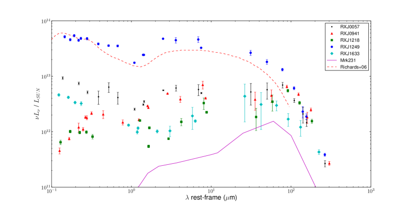
Figure 1: SEDs of our five QSOs, compared with a standard QSO template (Richards et al. 2006, dashed line, normalized to our most luminous object at $\sim$2000 Å) and the observed SED of Mrk 231 (a prototype ULIRG containing an AGN).

We have constructed the spectral energy distributions of all our objects, in $\nu L_{\nu}$ versus rest-frame wavelength in $\mu$m (Figure 1). We also show the observed SED (from NED) of Mrk 231: an ultraluminous infrared galaxy (ULIRG), without any renormalization. The average type 1 QSO template of Richards et al. (2006) is shown too. They constructed the SED from 259 quasars with SDSS and Spitzer photometry, supplemented by near-IR, GALEX, VLA and ROSAT data, where available. We have rescaled this template to be close to the observed SED of our brightest object (RX J1249), whose UV-FIR shape it closely matches.

All objects clearly show at least two components: UV-NIR contribution attributable to direct accretion disk emission (as expected from their type 1 nature), intrinsically absorbed in the cases of RX J0941 and RX J1218; and a reprocessed thermal component in the MIR region from warm optically thick dust further away from the nucleus (the torus). In all of them we also observe an additional FIR/submm component associated to cooler dust, heated by star formation (SF). We thus confirm the presence of strong FIR emission due to SF in these objects, at the ULIRG/HLIRG level (compared to e.g. Mrk 231).

3.1 Fit models

Our next goal is to make fits to our data with different templates to extract quantitative information about our objects. We use relatively simple empirical and theoretical templates, aiming at reproducing the general shape of the SEDs of our objects. We do not attempt to extract detailed physical information about our objects from those templates, since our data do not warrant such undertaking, and the underlying physics is likely to be more complex than that considered in the models. We have selected the Sherpa: CIAO’s modeling & fitting package (Freeman, Doe, & Siemiginowska, 2001) module for the Python platform (Doe et al., 2007) to perform the fitting. SEDs were fitted in $\nu L_{\nu}$ versus rest-frame $\lambda$. We have fitted only rest-frame wavelengths longer than 1218 Å, to avoid issues with the Ly-$\alpha$ forest. We have corrected for extinction in our Galaxy using the $A(\lambda)/A(V)$ values from Table 21.6 in Cox (2000) in the observer frame, assuming $R_{V}=3.1$ and $A(V)/N(H)\sim 5.3\times 10^{-22}$ cm^-2, extrapolating for wavelengths longer than 250 $\mu$m assuming $A(\lambda)\propto\lambda^{-2}$.

We have modelled the distinct constituents that can be appreciated in the SEDs of our objects (see above and Figure 1) with three different components:

• An AGN accretion disk component: This template models the direct emission from the accretion disk of the AGN (sub-parsec scales). We use the pure disk newAGN4 template from Rowan-Robinson et al. (2008), affected by intrinsic extinction (see below). The only free parameter is the normalization of the template. We have normalized the template to its integral in the 0.12-100 $\mu$m range (standard limits used to estimate the accretion disk luminosity). From the fits we directly obtain the value of the disk luminosity in that range, $L_{DISK}$.

• A torus component: This template models the re-emission from the warm and hot dust (on tens of parsecs scales, beyond the sublimation radius, see Antonucci 1993) that is warmed by the accretion disk emission. We have used both an empirical template from Rowan-Robinson et al. (2008) (dusttor, based on an average quasar spectrum) and three dusty clumpy torus models from Nenkova et al. (2008) found by Roseboom et al. (2013) to represent the average properties of type 1 QSOs (torus1, torus2 and torus3). The templates from Nenkova et al. (2008) have $N_{0}\sim 5-15$ dusty clouds along radial equatorial rays. The angular distribution of the clouds must have a soft edge, and the radial distribution decreases as $1/r$ or $1/r^{2}$.

  The difference of the latter model with the others is fundamentally that it has a higher inclination of the torus with respect to the line of sight (20 deg versus 0 deg), a larger number of absorbing clouds (by a factor of three) and a different distribution of the clouds (constant versus declining with distance as $1/r$).

  Similarly, we have normalized them to their integral in the 1-300 $\mu$m range (again, standard limits used for the torus luminosity), so the only free parameter is $L_{TORUS}$.

• A SF component: we have used a subset of the Siebenmorgen & Krügel (2007) spherical smooth models, found by Symeonidis et al. (2013) to encompass the observed SEDs of star-forming galaxies at least up to $z\sim 2$. The full Siebenmorgen & Krügel (2007) models have five free parameters to obtain their 7000 templates. The subset of templates recommended by Symeonidis et al. (2013) (around 2000 templates) are divided into 11 sub-grids, depending on the maximum radius and different star populations. For each source, we found the best-fit template for each of these 11 sub-grids. We did not attempt to extract detailed physical information from the particular best-fit templates, since instead we were looking for physically-motivated templates that reproduced the spectral shape of the data. Therefore, the only parameter that we obtained from these fits, apart from the best-fit templates, was the integrated FIR luminosity (40-500$\mu$m) $L_{FIR}$, since all templates were normalized in that spectral range. In addition, we have found the optically-thin greybody (GB) model (with free temperature $T$ and slope $\beta$) that best matches each best-fit SF templates at wavelengths longer than 40 $\mu$m rest-frame, providing two more “parameters” associated to each fit: $T$ and $\beta$.

The direct AGN accretion disk component was affected by intrinsic extinction modelled in terms of the hydrogen column density $N_{H}$, so that absorption $\propto\exp(-\sigma(\lambda)N_{H})$, where

$$\sigma(\lambda)={\log_{e}10\over 2.5}{A_{V}\over N_{H}}{A(\lambda)\over A(V)}$$ (3)

We have used $A_{V}/N_{H}=0.76\times 10^{-22}$ and the $A(\lambda)/A(V)$ values from the Gordon et al. (2003) SMC results for $\lambda<8100$ Å, and from Cox (2000) for longer wavelengths, both parametrizations merging smoothly at that wavelength.

In summary, we have 4 free parameters in the fits: the three luminosities ($L_{DISK}$, $L_{TORUS}$ and $L_{FIR}$) and the intrinsic extinction ($N_{H}$). In total, we have 44 (4 torus models $\times$11 SF models) possible combinations of all possible components and models.

We have minimized the usual $\chi^{2}$ statistics to choose between different models. Attending to the fact that there are many “hidden” parameters in our modelling (the different torus templates, and the many parameters in the Nenkova et al. 2008 and Siebenmorgen & Krügel 2007 models) and to the bad reduced $\chi^{2}$ values of our best fits ($2-135$), we have neither attempted to use the parameters of the absolute best-fitting template as the best value of the parameters, nor used $\Delta\chi^{2}$ to estimate the uncertainties in those. Instead, we have taken into account both the dispersion of the parameter values among models and the relative errors on the photometric points.

We have inspected the distribution of $\chi^{2}$ values for each source, finding that there were “families” of models that produced quite different values of that statistics. For each source (see below) we have chosen the family of models with the lowest $\chi^{2}$. Table 3 shows the average values of the luminosities and $N_{H}$ values among each best-fit family for each source and the minimum value of $\chi^{2}$ for each best-fit family. We have estimated the uncertainties in those values from the standard deviation.

Since have only included among those “families” one model for the direct AGN emission and only one or two models for the reprocessed AGN emission, the above dispersion gives rise to a unreasonably low uncertainty in the corresponding luminosities. Hence, we have used the average relative error on the relevant photometric points to estimate an additional relative uncertainty in all luminosities. We have calculated the average relative error in the rest-frame ranges 1218-10000 Å, 3-30 $\mu$m and $>100\,\mu$m for the direct AGN, reprocessed AGN and SF components, respectively. Those average relative values were multiplied by the corresponding average luminosities, finally adding them in quadrature to the above standard deviation.

We believe that these values and their uncertainties are fair estimates of the luminosities of each component and of the effects of the photometric errors and our lack of an accurate physical model for what is really happening in each source.

The shape of most of our SEDs in Figure 1 is very similar to the Richards et al. (2006) (R06) QSO template (UV-MIR region), but with an excess in the region of star formation (far-IR $/$submm region). So we have repeated the fits replacing the obscured disk and torus components, with intrinsic extinction, type 1 QSO SED template from Richards et al. (2006), keeping the SF component (a total of 11 sub-grids per fit). We have obtained $\chi^{2}$ values and FIR luminosities which are quite similar and compatible with the previous three-component ones. From these results we can draw two main ideas:

• The shape of our objects is well modelled (except perhaps for RX J1633, see below) by the Richards et al. (2006) template (UV-MIR region) and SF component, with some intrinsic extinction in two cases: they do not appear to be unusual in the UV-MIR region. Fits with separate disk and torus components are similarly good. In what follows we quote the latter results because they allow a more straightforward estimation of the direct and reprocessed AGN emission, and because they are clearly better for RX J1633.

• There is an excess in the far-IR $/$submm region that does not look like emission from the torus, indeed it is fitted very well with SF templates. We obtain quite similar FIR luminosities using accretion disk and torus models together or Richards et al. (2006) template.

On the other hand, all of our objects (except RX J1633) prefer the torus models dusttor, torus1 and torus2 which have similar shape. However RX J1633 clearly prefers the torus3 model. This torus model is one of the most extreme from Nenkova et al. (2008) with respect to the cold gas emission: it has a peak at higher wavelengths, but it is not enough to model our excess in far-IR $/$submm region. Summarizing, this (together with the discussion at the beginning of the Section 3.5) reinforces our idea that the excess far-IR $/$submm region corresponds to SF emission and not to the reprocessed AGN emission.

In the following, we have used the full three component fits for all QSOs because they treat the direct and indirect AGN components separately, allowing a comparison between them.

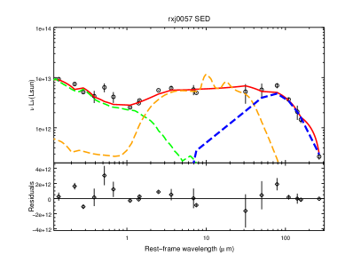
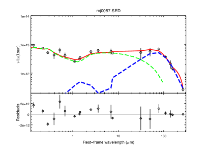
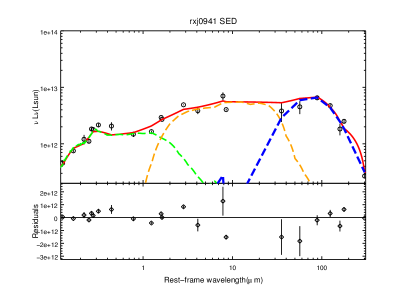
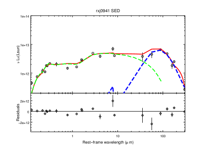
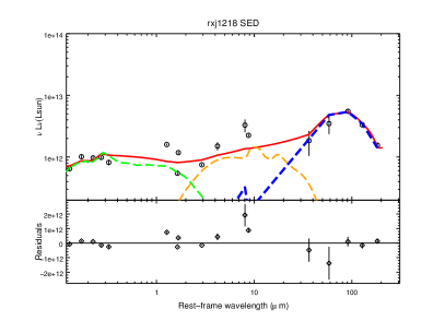
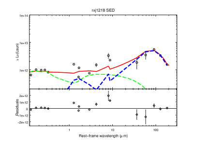
Figure 2: Best-fit SEDs to each source (one row per source) in two columns: on the left separate direct AGN (green dashed line), reprocessed AGN (torus, orange dashed line) and SF (blue dashed line) components; on the right, total AGN R06 (green dashed line) and SF (blue dashed line) components. We also indicate for each source which is the best-fit torus model. First row: RX J0057: Torus1. Second row: RX J0941: Dusttor. Third row: RX J1218: Torus2. Fourth row: RX J1249: Torus1. Fifth row: RX J1633: Torus3.

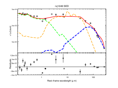
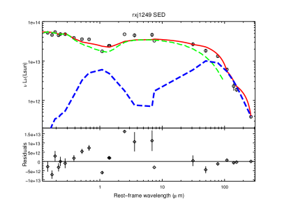
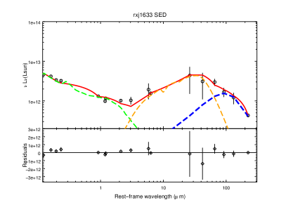
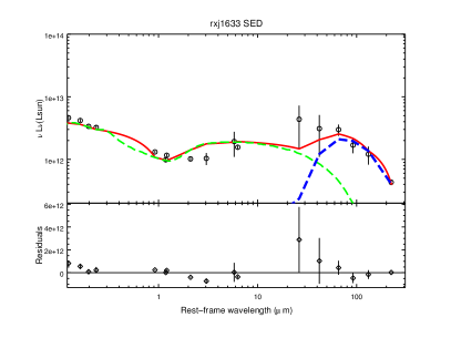
Figure 3: continued

Table 3: Average results and their uncertainties of fit parameters for each QSO, except for the X-ray AGN luminosity $L_{X,AGN}$ which comes from Page et al. 2011. $\chi^{2}$ represents the minimum value for each best-fit family and $N$ represents the number of photometric points that we have for each object.

Object	$L_{X,AGN}$	$N_{H}$	$L_{DISK}$	$L_{TORUS}$	$L_{FIR}$	$L_{IR}$	$T$	$\beta$	$\chi^{2}$ / N
	($10^{11}L_{\odot}$)	($10^{20}\,cm^{-2}$)	($10^{11}L_{\odot}$)	($10^{11}L_{\odot}$)	($10^{11}L_{\odot}$)	($10^{11}L_{\odot}$)	(K)
RX J0057	2.93	$0.01\pm 0.05$	$125\pm 17$	$190\pm 30$	$49\pm 10$	$170\pm 40$	$38\pm 4$	$1.1\pm 0.2$	159 / 20
RX J0941	0.93	$0.77\pm 0.11$	$100\pm 10$	$150\pm 20$	$78\pm 11$	$180\pm 30$	$36\pm 3$	$1.2\pm 0.2$	347 / 23
RX J1218	2.33	$0.39\pm 0.08$	$42\pm 7$	$25\pm 5$	$63\pm 6$	$90\pm 19$	$36.0\pm 1.7$	$1.2\pm 0.2$	414 / 17
RX J1249	3.69	$0.14\pm 0.03$	$1230\pm 90$	$1160\pm 100$	$70\pm 15$	$780\pm 90$	$39\pm 4$	$1.2\pm 0.2$	3109 / 23
RX J1633	5.85	$0.003\pm 0.002$	$65\pm 6$	$70\pm 30$	$22\pm 5$	$90\pm 30$	$36\pm 2$	$1.00\pm 0.11$	29 / 17

Table 4: Additional physical quantities derived from the average values and their uncertainties of the best-fit parameters.

Object	$L_{BOL}$	CF	$SFR$	$M_{DUST}$	$\Lambda_{EDD}$	$\dot{M}$	$k_{BOL}$
	($10^{11}L_{\odot}$)		($M_{\odot}y^{-1}$)	($10^{9}M_{\odot}$)
RX J0057	$250\pm 30$	$0.78\pm 0.15$	$840\pm 170$	$2.5\pm 0.8$	$0.09_{-0.07}^{+0.05}$	$17\pm 2$	$85\pm 10$
RX J0941	$169\pm 13$	$0.87\pm 0.14$	$1350\pm 190$	$4.1\pm 1.3$	$0.09_{-0.08}^{+0.05}$	$11.5\pm 0.9$	$182\pm 14$
RX J1218	$78\pm 7$	$0.32\pm 0.07$	$1090\pm 100$	$4.6\pm 1.6$	$0.13_{-0.12}^{+0.08}$	$5.3\pm 0.5$	$33\pm 3$
RX J1249	$1890\pm 90$	$0.61\pm 0.06$	$1200\pm 300$	$3.8\pm 0.9$	$0.61_{-0.6}^{+0.4}$	$128\pm 6$	$512\pm 8$
RX J1633	$186\pm 15$	$0.40\pm 0.16$	$380\pm 90$	$2.0\pm 0.7$	$1.1_{-0.9}^{+0.6}$	$12.6\pm 1.0$	$32\pm 3$

3.2 Luminosities from SED fits

We show in Table 3 the average value of the 8-1000 $\mu$m luminosity $L_{IR}$, calculated by integrating the torus and SF templates in that range and adding both contributions. Its uncertainty has been calculated in a similar way to those of the best-fit luminosities (see above), using both the standard deviation among the best-fit families and the relevant photometric errors (using this time the 8-1000 $\mu$m range), adding them in quadrature.

We define $L_{BOL}$ as the integrated 100 keV-to-100 $\mu$m luminosity from the AGN. We estimate this quantity using the observed absorption-corrected 2-10 keV (obtained from XMM-Newton spectra in Page et al. 2011) and 0.12-100 $\mu$m luminosities of our objects. For wavelengths longer than 0.12 $\mu$m we have integrated the fitted disk template. At wavelengths shorter than 0.0035 $\mu$m (0.35 keV) we have approximated the source continuum emission by a power-law $L_{\nu}\propto\nu^{-1}$, normalized to the observed absorption-corrected 2-10 keV luminosities (Page et al., 2011). Between those two wavelengths we have interpolated linearly in log-log (equivalent to assuming a power-law shape). Most of the final bolometric luminosity comes from the disk component (50-70 percent, except for RX J1633, for which this is 34 percent), so the exact parametrization of the higher energies does not have a strong influence on our results. We have calculated $L_{BOL}$ for each best-fit family, showing in Table 4 their average and its uncertainty, coming again from the dispersion among the best-fit families and the average relative photometric errors (using the same range as the one for the direct AGN component), adding them in quadrature.

3.3 Black Hole masses and related quantities from optical spectral fits

We have estimated the BH masses of our objects from the MgII and CIV emission lines from the optical-UV spectra in Page et al. (2011). The latter is usually preferred in the literature over the former because it presents lower complexity and wider scatter. Unfortunately, MgII is only covered by our spectra for RX J0941; for this source we have estimated the BH mass using both lines, to gauge the difference between using them. There are a number of different parametrizations of the BH mass as a function of the width of those lines and the luminosity in neighbouring wavelengths. We have chosen those used in Shen et al. (2011):

$$\log\left({M_{BH}\over M_{\odot}}\right)=2\log\left({FWHM\over 1000\,\mathrm{km/s}}\right)+$$

$$+0.50\log\left({\lambda L_{\lambda}\over 10^{44}\,\mathrm{erg/s}}\right)+6.86\,$$ (4)

for MgII (Vestergaard & Osmer, 2009), and

$$\log\left({M_{BH}\over M_{\odot}}\right)=2\log\left({FWHM\over 1000\,\mathrm{km/s}}\right)+$$

$$+0.53\log\left({\lambda L_{\lambda}\over 10^{44}\,\mathrm{erg/s}}\right)+6.66\,$$ (5)

for CIV (Vestergaard & Peterson, 2006), with rms values of 0.55 and 0.36 dex, respectively.

Table 5: Black hole masses from fits to the CIV line at 1548Å(except for the row marked with *, which comes from a fit to MgII at 2798Å), FWHM corresponding with each line, $\lambda F_{\lambda}$ the monochromatic luminosity corresponding with each line and the Eddington luminosity.

Object	FWHM	$\lambda F_{\lambda}$	$\log(M_{BH})$	$\log(L_{EDD})$
	(Å)	($10^{44}$erg/s)	($\log(M_{\odot})$	($\log(L_{\odot})$)
RX J0057	146$\pm$3	419$\pm$ 18	9.94$\pm$0.36	14.45$\pm$0.36
RX J0941	113$\pm$24	322 $\pm$29	9.77$\pm$0.40	14.27$\pm$0.40
RX J0941*	106$\pm$7	202 $\pm$18	9.22$\pm$0.55	13.72$\pm$0.55
RX J1218	77$\pm$23	150 $\pm$28	9.28$\pm$0.45	13.79$\pm$0.45
RX J1249	86$\pm$26	3731$\pm$392	9.99$\pm$0.45	14.49$\pm$0.45
RX J1633	53.9$\pm$1.2	178 $\pm$6	8.73$\pm$0.36	13.24$\pm$0.36

To obtain the $FWHM$ of the MgII and CIV lines, we have followed the technique outlined in Shen et al. (2011), which we summarize here. For MgII we have fitted, over the 2700-2900 Å rest-frame range, one narrow Gaussian component with $FWHM({\mathrm{k}m/s})=\max(\Delta\lambda,500)$ where $\Delta\lambda$ is the spectral resolution as given in Page et al. (2011) and one broad component, plus four Fe “humps” at rest-frame wavelengths of 2630, 2740, 2886 and 2950 Å. The continuum has been modelled as the best-fit power-law over the rest-frame range 2200-2700 Å (since the additional 2900-2090 Å range is not covered in our spectrum of RX J0941). For CIV we have fitted three Gaussians (only one was necessary for RX J0941) over the range corresponding to the expected position of CIV at the redshift of the source $\pm 20000\,{\mathrm{k}m/s}$, forcing their central wavelengths to be in the range 1500-1600 Å. The continuum has been modelled as the best-fit power-law over the rest-frame ranges 1445-1465 and 1700-1705 Å, see Figure 4.

In addition, the spectra of our sources presented a number of narrow and broad absorption lines, which we have modelled as multiplicative absorbing Gaussians $M(\lambda)=\left(1-A\exp\left(-{(\lambda-\lambda_{0})^{2}\over 2\sigma^{2}}\right)\right)$ with $0\leq A\leq 1$. We needed 3, 5, 7, 3 and 6 such components for RX J0057, RX J0941, RX J1218, RX J1249 and RX J1633 (respectively) around CIV, and 2 for RX J0941 around MgII.

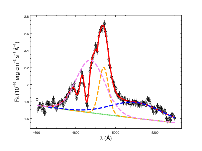
Figure 4: An example of the fits made to estimate the FWHM of the CIV emission line. We have modelled this feature for RX J0057 with three additive Gaussians (blue, orange and violet dashed lines), a power-law continuum (dotted green line) and three absorbing Gaussians (not shown individually). The total best-fit model is shown as a red solid line.

For RX J0941 we have obtained the $1-\sigma$ uncertainty on the $FWHM$ directly from that of the $\sigma$ of the single broad line fitted to the MgII and CIV lines, obtained in turn from the $\Delta\chi^{2}=1$ interval around the best fit value. Unfortunately, for the rest of the sources this is not so straightforward, since the CIV emission is modelled as the sum of three Gaussians, and there is no analytic expression relating the overall $FWHM$ to the best fit parameters of those three Gaussians (nine in total: three each of central wavelength, width and normalization). We have therefore sampled the parameter space, fixing those nine parameters to values around the best-fit ones, calculating the best-fit to each spectrum in the above range with the above constraints, calculating the $FWHM_{i}$ for each of those combinations of parameters, and assigning to each a probability $P_{i}=e^{(-\Delta\chi^{2}/2)}$ (Press et al. 1992). We have then estimated the variance on the $FWHM$ as $\sigma^{2}_{FWHM}=\langle FWHM-\langle FWHM\rangle\rangle\sim\sum_{i}P^{\prime}_{i}(FWHM_{i}-\langle FWHM\rangle)^{2}$ where $\langle FWHM\rangle\sim\sum_{i}P^{\prime}_{i}FWHM_{i}$ and $P^{\prime}_{i}=P_{i}/\sum_{i}P_{i}$ (to normalize the total probability to unity). For the sampling of each parameter we have used a Gaussian centred on the best-fit value with a dispersion set to (in decreasing order of choice) either the corresponding value of the covariance matrix (if defined), or to the $\Delta\chi^{2}=1$ interval (if defined), or to 10% of the best-fit value (1% in the case of the central wavelengths). The latter percentages were the rough averages of the dispersions of the similar parameters when they were defined. In any case, we checked that the final result did not depend on the particular choice of these dispersions, since they only serve to increase the efficiency of the sampling, favouring values close to the best-fit, where the highest probabilities should concentrate. We sampled 2000 combinations of parameters for each spectrum. We also checked that the dispersions did not depend on the exact number of sampling points.

The estimates of the continuum values $\nu L_{\nu}$ in the Eqs. 3.3, 3.3 (at rest-frame wavelengths of 1350 and 3000Å for CIV and MgII, respectively) have been obtained from the disk component that best fitted the overall SED of each source (see Section 3.1), which should provide a good estimate of the intrinsic disk emission, corrected for absorption. We have estimated the $1-\sigma$ uncertainties on those values from the dispersion in the values of the normalization of that component $L_{DISK}$ (see Section 3.1).

Finally, the uncertainties in $\log(M_{BH}/M_{\odot})$ have been estimated from those of $FWHM$ and of the continuum using the standard error propagation rules on the equations above (Bevington & Robinson 1992). We have added in quadrature the rms values in the equations above to get our rather conservative estimates of the total uncertainties. The BH mass estimates and the total uncertainties are given in Table 5. For RX J0941 we get $\log(M_{BH}/M_{\odot})=9.8\pm 0.4$ from CIV and $\log(M_{BH}/M_{\odot})=9.2\pm 0.6$ from MgII, which are within their mutual errors.

From the mass of the black hole we can calculate the Eddington luminosity using Eddington (1913):

$$L_{EDD}=3.2\times 10^{4}\frac{M_{BH}}{M_{\odot}}L_{\odot}$$ (6)

3.4 AGN-related quantities from SED fits

Once we have $L_{BOL}$ we can estimate naively the covering factor. Due to the anisotropy of the torus radiation we can only estimate the bolometric covering factor or apparent covering factor (Mor, Netzer, & Elitzur, 2009; Hönig et al., 2014) $CF$ as the ratio between the reprocessed emission from the torus and the total AGN bolometric luminosity:

$$CF=\frac{L_{Torus}}{L_{BOL}},$$ (7)

This gives us a measure of how much of the sky seen from the central source is intercepted by the torus. The values, shown in Table 4, have been calculated from the average values of $L_{TORUS}$ and $L_{BOL}$ and their uncertainties, using the standard propagation of errors.

The Eddington ratio would then be $\Lambda_{EDD}=L_{BOL}/L_{EDD}$. We show the values of $\Lambda_{EDD}$ in Table 4; they span the range $\sim 0.1-1.1$. The error bars on $L_{BOL}$ are symmetric in linear space, while those of $\log M_{BH}$ are large and symmetric in log space. The usual propagation of errors rules are only formally valid for small errors and using them would result in symmetric error bars for $\Lambda_{EDD}$ larger than the actual values. This does not make sense, since both the bolometric luminosity and the black hole mass are very significantly detected. To avoid these difficulties, we have estimated the uncertainties on the Eddington ratios sampling 10000 times the distribution of $L_{BOL}$ and $\log M_{BH}$ using Gaussians with the observed values, calculating the corresponding Eddington ratios, and finding the narrowest interval that included 68.3 percent of the sampled values. The resulting asymmetric error bars are those shown in Table 4.

3.5 Star-formation-related quantities from SED fits

Our SEDs require a contribution from cold dust, quantified by $L_{FIR}$. We have used the luminosities obtained in the previous Sections (given in tables 3.2 and 4) to check whether that cold dust could be powered by the AGN, following a simple energetic argument. We have compared $L_{BOL}$ (the total AGN power available) with $L_{TORUS}$ (AGN power already intercepted by the ”warm” reprocessing medium -the torus-) and $L_{FIR}$ (the observed power from cold dust): if $L_{BOL}$ is significantly larger than the sum of $L_{TORUS}$ and $L_{FIR}$, the AGN would have enough power to generate all the observed emission (with some to spare for the, mostly unobscured, observed UV-to-optical range). This can also be verified visually by looking at the SEDs in Fig. 2. It is clear that the AGN emission would be insufficient in RX J0057, RX J0941 and RX J1218. We have already discussed that the preferred torus model for RX J1633 includes a larger contribution from colder gas, producing a lower LFIR, so some of the putative AGN contribution would be already corrected for. As we will see below, RX J1249 is an exceptionally luminous QSO. However, its FIR emission is comparable to that of the other members of our sample, which would be unexpected it a significant contribution to that range came from such a powerful AGN. Concluding, the FIR emission observed in our objects likely predominantly comes from SF, as obviously it’s not just star-formation.

The SFR has been calculated from $L_{FIR}$ using the following expression from Kennicutt (1998),

$$SFR(M_{\odot}/\mathrm{y})=1.7217\times 10^{-10}L_{\mathrm{FIR}}(L_{\odot}),$$ (8)

We obtain values of $SFR\sim 1000M_{\odot}/\mathrm{y}$ (shown in Table 4). We confirm then our qualitative impression from Fig, 1: these objects are forming stars copiously.

Supernovae and binary stars associated with star formation produce X-rays. Symeonidis et al. (2011) found a tight correlation between X-ray luminosity and IR luminosity from ULIRGs, which can be expressed as $L_{X,SF}=(1.9\times 10^{26})L_{IR}^{0.3}+(4.15\times 10^{-5})L_{IR}$ (their equation 3). For the typical values of our QSOs of $L_{IR}\sim 10^{46}$, this corresponds to $L_{X,SF}\sim 10^{42}$ erg/s. Comparing these values with the AGN X-ray luminosities in the same band ($L_{X-AGN}\sim 4-20\times 10^{44}$ erg/s), we conclude that the contribution of the SF to the X-ray luminosity is very small and can be neglected.

In order to estimate the values of the dust mass associated with star formation, we have used the values of $L_{FIR}$, and the $T$ and $\beta$ obtained in Section 3.1 for each of the “good” sub-grids. We have related those three quantities to the dust mass $M_{DUST}$ using Equations 2 and 5 in Martínez-Sansigre et al. (2009). Their Equation 2 can be written as

$$L^{\prime}_{\mathrm{FIR}}={8\pi h\over c^{2}}{d_{L}^{2}(z)F_{\nu^{\prime}}\over(1+z)(\nu^{\prime}(1+z))^{\beta}B_{\nu}(T,\nu^{\prime}(1+z))}{1\over F}$$ (9)

where $F_{\nu^{\prime}}$ is the observed monochromatic flux at some reference observed frequency $\nu^{\prime}$ (in their case $\lambda^{\prime}=1.2$ mm), where

$$F=\int_{0}^{\infty}d\nu\frac{\nu^{3+\beta}}{\exp(h\nu/kT)-1}={\Gamma(\beta+4)\zeta(\beta+4)\over\left({h\over kT}\right)^{\beta+4}}$$ (10)

((Gradshteyn et al., 2007) FI II 792a) is the normalization of the greybody function to the full frequency range. Eq. 9 is simply the total luminosity of a greybody normalized to the observed value of $F_{\nu^{\prime}}$. We have called this quantity $L^{\prime}_{FIR}$ to emphasize the difference between this and the usual definition of $L_{FIR}$ over the 40 to 500 $\mu$m range.

Similarly, Eq. 5 in Martínez-Sansigre et al. (2009) can be written as

$$M_{\mathrm{DUST}}={d_{L}^{2}(z)F_{\nu^{\prime}}\over(1+z)\kappa(\nu^{\prime}(1+z))B_{\nu}(T,\nu^{\prime}(1+z))},$$ (11)

where

$$\kappa(\nu(1+z))=\kappa_{0}\times\left({\nu(1+z)\over\nu^{\prime}}\right)^{\beta},$$ (12)

We have used $\kappa_{0}=0.04$ m²/kg at $\lambda^{\prime}=$1.2 mm (Beelen et al., 2006). If we now divide Eq. 11 by Eq. 9, substituting Eq. 10, we get

$$M_{DUST}={c^{2}\over 8\pi h}{1\over\kappa_{0}\nu^{\prime-\beta}}{L^{\prime}_{FIR}\over\int_{0}^{\infty}d\nu\frac{\nu^{3+\beta}}{\exp(h\nu/kT)-1}}$$ (13)

where the last fraction is simply a normalization over the full frequency range.

We have instead used

$$M_{DUST}={c^{2}\over 8\pi h}{1\over\kappa_{0}\nu^{\prime-\beta}}{L_{FIR}\over\int_{40\,\mu\mathrm{m}}^{500\,\mu\mathrm{m}}d\nu\frac{\nu^{3+\beta}}{\exp(h\nu/kT)-1}}$$ (14)

using the usual definition of $L_{FIR}$, which we have obtained directly from our SED fits. We show in Table 4 the averages and standard deviations of the acceptable families of models. Our approach involves two approximations: replacing the renormalization over the full interval to that over the 40 to 500 $\mu$m interval, and replacing the FIR luminosity from a greybody with that from a fit to a more sophisticated SF model. We believe that we are justified to do both because, on the one hand, the greybody shape decreases very fast outside the usual FIR range and, on the other hand, the integrals over that range of the greybody fits to the SF templates gave very similar values to those of the actual templates.

We can also estimate the gas mass present in the starforming regions of those galaxies from the dust masses, assuming a gas-to-dust ratio of 54, deduced by Kovács et al. (2006) for $z=1-3$ SMG (with an uncertainty of about 20 per cent). This value is similar to the one obtained by Seaquist et al. (2004) for the central regions of nearby submm bright galaxies. For our typical dust mass of $\sim 10^{9}M_{\odot}$ this corresponds to a gas mass of $M_{GAS}\sim 10^{10}-10^{11}\,M_{\odot}$.

3.6 Time scales

Assuming an efficiency in conversion of accreted mass into radiation $\eta$ (we have assumed 10% e.g. Treister & Urry 2006) the mass accretion rate $\dot{M}$ can be related to the bolometric luminosity $L_{BOL}$ by:

$$L_{BOL}=\eta\dot{M}c^{2}$$ (15)

The relative speed of galaxy-building through star formation and black hole growth through accretion can be estimated from $SFR/\dot{M}$. Both quantities are included in Table 4, with errors derived using the standard propagation of errors.

Assuming a constant accretion rate, we can estimate the black hole mass doubling time $\tau$ as

$$\tau\sim\frac{M_{BH}}{\dot{M}}$$ (16)

and, defining the maximum mass of the black hole as $M_{BH,max}$ (which we take as $2\times 10^{10}\,M_{\odot}$, the maximum value of the observed black hole masses in the local Universe, NGC 4889, from column 10 in Table 2 of Kormendy & Ho 2013, McConnell et al. 2012), the time $\tau_{max}$ needed to reach it is

$$\tau_{max}\sim\frac{M_{BH,max}-M_{BH}}{\dot{M}}$$ (17)

Alternatively, we could have used in the numerator of Eq. 17 simply $M_{BH,max}$, but the masses of the black holes in the centres of our objects are already comparable to the maximum local black hole mass, so Eq. 17 is more accurate. We have again sampled the distribution of $\dot{M}$ and $\log M_{BH}$ to estimate the uncertainties in these two timescales, as discussed above.

Assuming again a maximum local black hole mass, we can estimate what would be its corresponding maximum host galaxy mass, $M_{BULGE,max}=8.53\times 10^{12}\,M_{\odot}$, using the Marconi & Hunt (2003) relation. From that value and the current SFR observed in our objects, assuming again constant SFR, we can estimate the time $\tau_{SB}$ needed to reach that maximum mass value as:

$$\tau_{SB}\sim\frac{M_{BULGE,max}}{SFR}$$ (18)

The values of all these timescales are shown in Table 6, along with the time between their epochs and now (“look-back time” ).

Table 6: Summary of timescales for QSOs and star formation, assuming constant mass accretion rates and SFR. $\tau$ is the black hole mass-doubling timescale, $\tau_{max}$ is the time needed to reach the maximum local black hole mass (see text), and $\tau_{SB}$ is the time needed to reach the corresponding maximum host galaxy mass. $t$ is the “look-back time” (see text).

Object	$\tau$	$\tau_{max}$	$\tau_{SB}$	$t$
	$(Gy)$	$(Gy)$	$(Gy)$	$(Gy)$
RX J0057	$0.5_{-0.4}^{+0.3}$	$0.7_{-0.4}^{+0.4}$	$10\pm 2$	10.6
RX J0941	$0.5_{-0.5}^{+0.3}$	$1.2_{-0.4}^{+0.5}$	$6.3\pm 0.9$	10.0
RX J1218	$0.4_{-0.3}^{+0.2}$	$3.4_{-0.5}^{+0.5}$	$7.8\pm 0.7$	9.9
RX J1249	$0.08_{-0.07}^{+0.05}$	$0.08_{-0.06}^{+0.07}$	$7.1\pm 1.8$	10.6
RX J1633	$0.04_{-0.04}^{+0.02}$	$1.55_{-0.15}^{+0.11}$	$22\pm 5$	11.3

4 Discussion

In this Section we will piece together the clues obtained above about the nature of our objects.

From the SED shapes and template fits, we see some differences in the properties of the objects in our sample: RX J0057 and RX J1249 have similar redshifts $z\sim 2.2$, small optical obscurations, the highest bolometric AGN luminosities and a preference for the first torus model in Roseboom et al. (2013). RX J0941 and RX J1218 have again similar redshifts $z\sim 1.8$, higher optical obscurations, the lowest bolometric AGN luminosities and also allow for the empirical Rowan-Robinson et al. (2008) and the second Roseboom et al. (2013) torus models. Finally, RX J1633 has the highest redshift $z=2.8$, small optical obscuration, intermediate bolometric AGN luminosity and a strong preference for the third torus model in Roseboom et al. (2013). This results in a higher torus contribution at longer wavelengths, intuitively corresponding to a higher probability of further reprocessing of the direct emission at larger distances and lower temperatures. Additional evidence for a (relative) higher inclination of RX J1633 comes from its radio morphology in FIRST images, which shows two diffuse blobs roughly symmetrical with respect to the optical position of the QSO, in contrast with the rest of our objects, which are either not detected (RX J0057 and RX J1218) or pointlike (RX J0941 and RX J1249).

The host galaxies of RX J0941 and RX J1218 seem to be growing much faster than their black holes, both in absolute terms and compared to the other objects. This is because their AGN are less luminous but have similar $SFR$ to the rest. The difference in AGN luminosities between the objects could be ascribed to the redshift, since those further away are also more luminous, as expected in a flux-limited sample, but this is belied by the intermediate luminosity of the highest redshift object RX J1633, which is also the one with the most discordant torus properties. In any case, with such a small sample it is impossible to assess the significance and implications of the differences observed.

4.1 AGN properties

In this section we want to study the main properties of the AGN. Taking the sample as a whole, we can compare their overall properties to those of type 1 QSO from the SDSS DR7 (Abazajian et al., 2009): bolometric luminosities (Shen et al., 2011), Eddington luminosities and ratios (Kelly & Shen, 2013) and covering factors (Roseboom et al., 2013).

As expected from the design of the sample (Page, Mittaz, & Carrera 2000), their X-ray and bolometric luminosities are similar to those of QSOs in their redshift ranges (using a range $\Delta z=0.4$), except for RX J1249, which is truly exceptional: there are only 50 objects brighter than RX J1249 ($<$0.05%) in the whole sample of Shen et al. (2011), and it is one of the most luminous object even comparing with the high-bolometric-luminosity-selected sample of Tsai et al. (2014). Also, as discussed above, the shape of their SEDs in the optical-MIR region is unexceptional.

From Table 4, three of our QSOs have Eddington ratios around 0.1 (RX J0057, RX J0941 and RX J1218), one has a value around 0.6 (RX J1249) and the last one is closer to unity (RX J1633), although with large error bars, specially in the last two. This range of values is compatible with that found by Kelly & Shen (2013), who have studied a sample of $\sim$ 58000 Type 1 QSO, also finding that $\Lambda_{EDD}\lesssim 0.1$ are significantly rarer at $z\sim 4$ compared to $z\lesssim 2$, while objects with $\Lambda_{EDD}\gtrsim 0.1$ are found similarly in both redshift ranges. This is also similar to what we see in our sample, where the four objects with $z\sim 2$ are compatible with $\Lambda_{EDD}\sim 0.1$, while RX J1633 at $z=2.8$ shows some preference for higher values of $\Lambda_{EDD}$. They conclude that Type 1 quasars radiating near the Eddington limited are extremely rare, suggesting that Type 1 quasars violating the Eddington limit do so only for a very brief period of time. RX J1633 could be in this situation.

Roseboom et al. (2013) have estimated the covering factors $CF$ of their WISE-UKIDSS-SDSS (WUS) quasar sample (5281 quasars) with $z<1.5$. They have found an average value of $CF=0.39$, but in addition they also get that two-thirds of type 1 quasars have $CF$ in the range 0.25 to 0.61, roughly as in our sample. Segregating the sources according to their bolometric luminosities, our four lower luminosity objects are in their $46<\log(L_{BOL})<47$ bin. A quick MonteCarlo sampling of the log-normal fit to their $CF$ distribution (calculating values from our sample with respect to the mean values of the distribution and five random distribution values with respect to the mean values too) shows than an unremarkable 40 per cent of the simulated samples have a similar distribution as our objects in this bin. In contrast, RX J1249 is in their highest luminosity bin ($\log(L_{BOL})\sim 48$), where only three percent of the objects have a higher $CF$ than this source: RX J1249 is not only one of the most luminous objects known, it also has an exceptionally high reprocessed-to-bolometric AGN luminosity ratio for its luminosity.

We have calculated the bolometric corrections to the X-ray luminosities for our sample defined as:

$$k_{BOL}=\frac{L_{BOL}}{L_{X,2-10}}$$ (19)

finding values $k_{BOL}\sim 30-500$ (see Table 4) for $\Lambda_{EDD}\sim 0.1-1$. Although at face value this looks very different from the results of Vasudevan & Fabian (2009), our three objects with $\Lambda_{EDD}\sim 0.1$ (RX J0057, RX J0941 and RX J1218) are well within the values spanned by the objects in their sample at similar Eddington ratios $k_{BOL}\sim 30-180$ (see their Fig. 6). The most discrepant objects are RX J1249 and RX J1633. The former presents an extremely high bolometric correction around 500, more in line with its BAL nature (Grupe, Leighly, & Komossa, 2008; Morabito et al., 2014). On the contrary, RX J1633, our highest redshift object, presents a bolometric correction of about 30 for an Eddington ratio of about 1. Only one object from Vasudevan & Fabian (2009) has a smaller correction for that ratio, although there are a few more with $\Lambda_{EDD}>0.1$ and $k_{BOL}\lesssim 40$ in their sample, so it is not exceptional. We have also compared our bolometric corrections with those of Marconi et al. (2004). Only RX J0057 is close to their relation and inside the dispersion region, RX J1249 and RX J0941 are above the relation and RX J1218 and RX J1633 are below the curve. Again the most discrepant sources are RX J1249 and RX J1633.

4.2 Star formation properties

Regarding now the star formation properties of our sample, we have obtained very high SFRs$\sim 1000M_{\odot}$/y: these objects are forming stars copiously and they are at the ULIRG/HLIRG level with strong FIR emission.

The distribution of greybody temperatures ($T=36-39$ K) of the SF templates of our sources seems to be closer to those of SMGs ($T\sim 35$ K, Beelen et al. 2006), than to those of other high redshift QSOs ($T\sim 47$ K, Kovács et al. 2006): the range of temperatures in the latter work is $T\sim 40-60$ K while only two of our sources have temperatures compatible with the lower bound of the interval (RX J0057 and RX J1249, the first subset discussed at the beginning of this section). On the other hand, we obtain greybody slopes ($\beta=1-1.2$) below those of typical SMG ($\beta=1.5$ Beelen et al. 2006) and high redshift QSOs ($\beta=1.6$ Kovács et al. 2006), even taking into account the substantial error bars. However, our temperatures and slopes could be affected by the limited wavelength range of the greybody fits to the SF templates, since the SF thermal bump in our sources is generally broader than in simple greybody models, and hence the fit tends towards low values of $T$ (to match the steep decline at the longest wavelengths) and low values of $\beta$, to accommodate the extra width at the shorter wavelengths. If we just use a simple greybody model to parametrize the SF, instead of the more elaborate templates of Siebenmorgen & Krügel (2007), we confirm the above tendency: both RX J0057 and RX J1249 prefer higher temperatures than in the limited-range-fit to the best-fit SF template, while the rest show similar or slightly lower temperatures. This would go in line with the fact that in the former two objects the maximum of the SF emission is lower than that of the torus emission, while in RX J0941 and RX J1218 the opposite happens. Finally, it might well happen that a single temperature fit without some modification at the high frequency end is not sufficiently accurate to allow a precise determination of $\beta$-T values. In any case, the exact values of those parameters in particular fits have a very limited impact in our inferred luminosities, since we derive quantities from averages and dispersions over the best group of fits.

4.3 AGN-SF relationship

In the context of possible evidence for an influence of the central AGN on the evolution of its host galaxy, it is interesting to compare the rate of black hole growth (as gauged from e.g. the X-ray luminosity $L_{X,2-10}$, the intrinsic bolometric luminosity from AGN $L_{BOL}$, or the accretion rate $\dot{M}$) to the rate of galaxy growth (from the SFR, the LIR or the monochromatic 60$\mu$m luminosity). Lutz et al. (2008) studied the correlation between $log(\nu L_{\nu}$) at 60$\mu$m and PAH emission (as proxies of the SF luminosity) and $log(\nu L_{\nu}$) at 5100Å(as a proxy for the AGN luminosity) for a sample of QSOs at similar $z$ to ours with Spitzer spectroscopic data in the rest-frame mid-infrared. They have found that, at high luminosities and $z$, there was a flattening of the relation between SF and AGN luminosity that is observed for lower redshift QSOs. Mullaney et al. (2012) used 100 and 160 $\mu$m fluxes from GOODS-Herschel finding no evidence of any correlation between the X-ray and infrared luminosities of moderate luminosity AGNs at any redshift. Rovilos et al. (2012) found a significant ($>$99%) correlation between $L_{X,2-10}$ and SFR (see Figure 5) in a deep GOODS-XMM-Newton-Herschel sample, taking into account the upper limits on the latter using the ASURV package (Lavalley, Isobe, & Feigelson 1992). They also found a significant correlation between the specific SFR (sSFR) and X-ray luminosity, taking into account both upper limits and a possible partial correlation with the redshift. Rosario et al. (2012) used the COSMOS-GOODS- North and South X-ray selected sample. They study $log(\nu L_{\nu}$) at 60$\mu$m vs. $L_{BOL}$ finding a significant correlation between $L_{\nu}$ at 60$\mu$m and $L_{BOL}$ for moderate redshifts ($z<1$) and high luminosities.

Interestingly, all our objects are in the redshift range ($1<z<3$) studied by Page et al. (2012). They studied Herschel SPIRE observations of the CDF-N field (within the HerMES project) and found evidence for star formation (from 250 $\mu$m detections) in some X-ray detected AGN with $10^{43}<L_{X,2-10}<10^{44}$ erg/s, but lower star formation in the $10^{44}<L_{X,2-10}<10^{45}$ erg/s luminosity bin. They took this as evidence for suppression of SFR in the most luminous AGN at that epoch in the Universe. Since all our objects are very significantly detected in 250 $\mu$m and have $L_{X,2-10}>10^{44}$ erg/s (see Fig. 5), in this scenario these highly luminous QSOs would not yet have managed to switch off SF.

In this controversial context, we have revisited the $\log(SFR)$ vs. $\log(L_{X,2-10})$ correlation using both their sample and a joint sample with our sources (including data from (Stevens et al., 2005)). We have tested for a “hidden” correlation with redshift (specifically with the luminosity distance $\log(d_{L})$) using the method in Akritas & Siebert (1996), who give their significance in terms of a ratio between the generalized Kendall’s $\tau$ and its dispersion $\sigma$.

We first started with just their sample, finding $\tau/\sigma=5.1$. We tested this significance against simulated samples of sources with mutually uncorrelated SFR and X-ray luminosity values, but both correlated with redshift. Briefly, we found the constants $K$ that best reproduced the $\log(Y)=K+2\log(d_{L})$ relations, with $Y=\log(SFR)$ (using only detections) and $Y=\log(L_{X,2-10})$, estimated the rms around these relations for several ranges of redshift, and then created 10000 samples of sources keeping the redshifts of the observed sources and simulating the X-ray luminosities and the SFR with the above “calibrations”. For upper limits in SFR we kept the observed upper limit but randomized the X-ray luminosity as above. These simulated samples keep the statistics of the Rovilos et al. (2012) sample but do not have any real correlation between SFR and X-ray luminosity. We found that 653 of those had $\tau/\sigma>5.1$, so we conclude that the real significance of the correlation in their sample is about $\sim 1-653/10000=93$%$<2\sigma$.

We now wish to add our sample to this relation to check its influence. We need to use our full parent sample in Stevens et al. (2005), including the non-detections at 850 $\mu$m. Note that there are three more “detections” in that paper compared to this paper: RX J1107+72 (because it is radio-loud and hence its FIR emission originates in the AGN), RX J0943+16 and RX J1104+35 (these two are $<3\sigma$ significant). The 0.5-2 keV luminosities in that paper (Stevens et al., 2005) have been converted to 2-10 keV luminosities assuming $L_{\nu}\propto\nu^{-1}$ (we have checked that this method agreed well with the 2-10 keV luminosities from (Page et al., 2011) used elsewhere in this work). For the five common sources, we have fitted the best multiplicative constant between the 850 $\mu$m-derived FIR luminosities in Stevens et al. (2005) and our SED-derived FIR luminosities, taking into account the uncertainties in both quantities. Using this multiplicative constant we have then derived “corrected” FIR luminosities and SFR (EQ. 8) for all sources in Stevens et al. (2005) sample (green points in Fig.5). The linked points show the magnitude of the re-scaling for the five common sources (red -this paper-, green -rescaled-). The rescaled full parent sample has been joined to the Rovilos et al. (2012) sample to study the X-ray luminosity-SFR correlation. Again, we have created 10000 random samples as explained above (re-calibrating the SFR and X-ray luminosity correlations with redshift and their rms). The joint sample gave $\tau/\sigma=5.61$. Only 23 out of 10000 random simulations showed higher values, so the significance is $\sim$99.8%$>3\sigma$. This joint correlation is more significant probably because our five detected sources extend the X-ray luminosity range by almost an order of magnitude.

At face value, it appears that there is a significant correlation between the growth of galaxies via star formation and the growth of their central SMBH via accretion in the joint sample. However, a number of caveats are in order to interpret the observed correlation. First, given the very different selection functions of the samples involved (between them and among their constituent surveys at different wavelengths) and the small numbers of sources involved, it is very difficult to assess the significance of the different results in terms of the full population of black-hole-growing and/or star-forming galaxies at that epoch in the Universe. Large samples of objects at the relevant redshifts with well-controlled selection functions are needed to appraise this crucial issue. Furthermore, our SED-derived SFR cover very well the FIR rest-frame range even at our highest redshift (as they include observed frame points between 100 and 850 $\mu$m) and the “corrected” ones used for the correlation come originally from observed-frame 850 $\mu$m observations (similar to Lutz et al. 2008). In contrast, the highest observed wavelength in Rovilos et al. (2012), Mullaney et al. (2012) and Rosario et al. (2012) is 160 $\mu$m, which only covers the short-wavelength side of the FIR bump at redshifts above 1, with the ensuing uncertainty in the FIR luminosities, despite the careful SED fit.

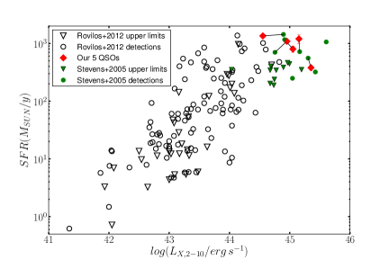
Figure 5: Star-formation rate versus X-ray luminosity for our five quasars (red solid diamonds, with values as reported in this paper). For comparison, we also show X-ray selected AGN in deep Herschel surveys from Rovilos et al. 2012: 99 FIR-detected (empty dots) and 32 with only FIR upper limits (empty triangles). We have also included data from our full parent sample in Stevens et al. 2005, modifying the X-ray luminosities and SFR to a frame coherent with the data in this paper (see text): detected sources (green solid circles, joining with a segment the points corresponding to the common sources) and upper limits (green solid triangles).

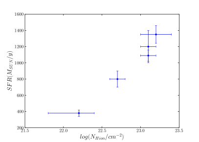
Figure 6: Star formation rate versus ionised column density N${}_{H_{ion}}$ for our sample. (from Page et al. 2011).

Previous works have found some evidence of a correlation between the SF of the host and the AGN obscuration by neutral gas in the X-rays (Alexander et al. 2005, Bauer et al. 2002, Georgakakis et al. 2004, Rovilos et al. 2007). Later studies with deeper surveys both in the X-ray and infrared ranges have failed to reproduce these results (e.g Rosario et al. 2012, Rovilos et al. 2012). We have therefore looked instead for a correlation between the ionised column density N${}_{H_{ion}}$ (from Page et al. 2011) and SFR in our sources (Fig. 6), finding a tentative positive correlation between these parameters. This is interesting, since it would imply a coupling of the ionized gas absorbing the X-rays at the scale of the accretion disk or the BLR with the gas forming stars in the host galaxy bulge, about three orders of magnitude farther away. At face value, this would be compatible with a positive feedback scenario, (King et al., 2013) in which the ionized outflowing gas would trigger star formation in the interstellar medium of the host galaxy, with the highest column density gas corresponding to stronger feedback.

Alternatively, the AGN may also be ionising gas at kpc scales, co-located with the SF gas, so the above correlation would just be a consequence of the gas of higher density forming stars more intensely. Testing this intriguing possibility (with implications on positive and negative feedback) would need larger samples with a better determination of the location of the ionised gas.

4.4 Evolutionary status

We now turn to the fate of the objects in our sample. Assuming constant accretion rates, we have estimated in Section 3.6 their BH mass-doubling times $\tau$ and the time they would take to reach the maximum BH mass observed locally $\tau_{max}$. We note that RX J0057, RX J0941 and RX J1249 are already within a factor of 2-3 of this maximum local BH mass ($\sim 2\times 10^{10}\,M_{\odot}$), so their BH growth phase is expected to finish within one to three mass-doubling times at most, i.e. 700, 1200 and 80 million years respectively. Given the expected lifetime of an active QSO phase of about 200 million years (Hopkins et al., 2008), RX J1249 would have time to reach that maximum mass, while the other two objects would stop at a lower, but not much lower, mass. The BH in the centre of RX J1633, the least massive in our sample (but already with a considerable mass of about $10^{9}\,M_{\odot}$, larger than about 60% of the objects in Marconi & Hunt 2003), is growing quite fast, doubling its mass in 40 million years, so it could increase its mass by a factor of a few within the fiducial QSO lifetime above. RX J1218 has a intermediate BH mass in our sample (about 10 times lower than the local maximum), but its accretion rate is the lowest in the sample, so its mass-doubling time is 3 Gy. Therefore, unless something happens to re-kindle the AGN at a later time, it is unlikely to grow much more.

Without a determination of the masses of the host galaxies of our objects we cannot perform a similar exercise for the expected lifetime of the starburst phase. Unfortunately, the UV-to-MIR range is completely dominated by the AGN light. We are trying to secure mm observations to estimate the host galaxy masses directly. Nevertheless, we can argue that the SFRs observed are very high (albeit with considerable uncertainties), among the highest observed at the relevant redshifts, so they are unlikely to be maintained for a long time.

Considering further episodes of strong galaxy growth with little AGN growth does not help to escape that the galaxies should be already formed, since either the host galaxy has to swallow whole fully-formed large-mass galaxies without forming stars (and with insignificant BH masses), or the ensuing SFR would have to be several times larger than the already extraordinary ones found in our objects (while at the same time avoiding a significant infall of gas to the galaxy nucleus to make sure to starve the massive BH already in place).

In an independent line of argument, in the event that there is a positive feedback at work, as discussed in Section 4.3, then the bulk of the gas mass in the host galaxies could be about to form stars pressured by the now maximal AGN, and so perhaps that could allow the BH-bulge relation to be reached quickly. However, this would be surprising, because the $\sim 10^{11}\,M_{\odot}$ of stars in an elliptical today typically seem to have formed at higher redshifts (Daddi et al., 2005).

In the context of co-evolution of AGN and their host galaxies, e.g. the recent recently proposed by Lapi et al. (2014), our objects, with $0.04<L_{FIR}/L_{BOL}<0.81$ would be in a stage when the FIR-luminous phase is close to end (Figure 15 in Lapi et al. 2014), in qualitative agreement with our conclusion that their host galaxies are already mostly formed.

5 Conclusions

We have studied a sample of X-ray-obscured QSOs at $z\sim 2$ with strong submm emission (Stevens et al., 2010), much higher than most X-ray-unobscured QSOs at similar redshifts and luminosities, which, however, represent 85-90 per cent of the X-ray QSOs at the epoch. We have built X-ray-to-FIR SEDs for each object and we have fitted them using different models (a direct AGN accretion disk, a torus-reprocessed component and a star formation component). We confirm that direct AGN, reprocessed AGN and SF components are needed to correctly characterize the SEDs of our objects. We have used these fits, together with our previous determinations of their X-ray luminosities, to estimate the total direct and reprocessed AGN luminosities and the luminosity associated to the star formation, as well as other derived physical quantities.

We confirm the presence of strong FIR emission in these objects (well above that expected from plausible AGN emission models) which we attribute to SF at the ULIRG/HLIRG level with SFR$\sim$1000 $M_{\odot}/$y. Their associated greybody temperature values are close to those of Submillimeter Galaxies (SMGs). They have dust masses around $10^{9}$ M_⊙.

We have found a just over 3-$\sigma$ significant correlation between the SFR and the X-ray luminosity when joining our sample with that from Rovilos et al. (2012). This is usually taken as evidence for joint AGN and galaxy growth, but the differences between the techniques used to detect and characterize SF in those two samples detract from this otherwise exciting, interpretation. Our objects fall in the high luminosity end of large samples from deep surveys (Rovilos et al., 2012; Rosario et al., 2012), but have similar properties to other samples of high $z$, high FIR luminosity objects (Lutz et al., 2008). However, RXJ1249 stands out in all cases: it is one of the most luminous objects known (bolometric luminosity $\sim 10^{48}L_{\odot}$) and it has an exceptionally high torus-to-bolometric luminosity ratio for its luminosity.

Comparing their AGN reprocessed and direct emission, we have obtained the ratios between the reprocessed emission from the torus and the total AGN bolometric luminosity $\sim 0.3-0.9$, higher than QSOs of similar luminosities at $z<1.5$. The Eddington ratios of our objects (0.1-0.6) are common for their redshift range, except for RX J1633 (our highest redshift object) which has a value of that ratio close to unity. Overall, the bolometric corrections of our objects do not fit well with those of other studies (Vasudevan & Fabian, 2009; Marconi et al., 2004), showing higher bolometric luminosities compared to their X-ray luminosities.

We have found a tentative positive correlation between NH_ion and SFR, perhaps indicative of positive feedback between the X-ray and UV-detected ionized outflowing gas and the interstellar medium of their host galaxies.

The black holes powering our QSOs are very massive at their epoch, $\sim 10^{9}-10^{10}M_{\odot}$ (measured from broad emission lines in their optical-UV spectra). We have calculated their mass-doubling timescale $\tau$ and the time to reach the maximum BH mass observed locally, concluding that they can not grow much more. A further hint in this direction comes from the high Eddington ratio of RX J1633 which, according to Kelly & Shen (2013) should persist only for a very brief period of time. RX J1249 could become one of the most massive objects known.

We do not know the masses of their host galaxies, but their black hole masses and their high SFR lead us to conclude that they are already very massive or they would not have enough time to reach the local bulge-to-black-hole-mass ratio. This is also in agreement with recent models of AGN-host galaxy co-evolution.

Direct determinations of the gas mass and of the mass of the host galaxies our QSOs are needed to have a better grasp of the nature and evolutionary status of these exceptional objects, and hence to understand their role in the disputed landscape of co-evolution of galaxies and AGN.

Appendix

We now discuss briefly the fit results for each source:

• RX J0057: We have chosen the first torus model family from Roseboom et al. (2013) (11 members), since the other fits gave $\chi^{2}$ values at least 40 per cent higher.

• RX J0941: We have selected the first torus model family from Roseboom et al. (2013) and the empirical template from Rowan-Robinson et al. (2008) (22 members). The other torus models from Roseboom et al. (2013) have $\chi^{2}$ values at least 30 per cent higher.

• RX J1218: Contrary to the other sources, the best-fit models were not visually good, since the $\chi^{2}$ value was dominated by the fits to the optical-to-MIR region (where the error bars are smallest), leaving the SF bump badly represented. For each disk+torus+SF combination we fixed the model parameters to their values best fitting the overall SED, and re-calculated the $\chi^{2}$ value restricted to the rest-frame band 36-190 $\mu$m (5 points). We found that this restricted $\chi^{2}$ had a clear best-fit peak with $\chi^{2}\leq 12$, including 20 disk+torus+SF combinations, with the rest of the combinations extending in a tail towards higher restricted $\chi^{2}$ values. We have chosen these 20 combinations as our best-fit “family”. Their torus components include both the first and second torus models of Roseboom et al. (2013), as well as the empirical template from Rowan-Robinson et al. (2008).

• RX J1249: This case is very similar to RX J0057: we have selected the first torus model family from Roseboom et al. (2013), for which the $\chi^{2}$ values were at least 40 per cent lower.

• RX J1633: The third torus model from Roseboom et al. (2013) produced a well-grouped family (11 members) of best-fits with low $\chi^{2}$ values. There were a few scattered best-fits with lower $\chi^{2}$ using other models but they showed systematic residuals around rest-frame 30-60 $\mu$m, with SF components taking over the torus contribution in that band. We have chosen that family as our preferred fit.

From the results, see Figure 2, above, it is clear that the first torus model of Roseboom et al. (2013) is preferred by two of our sources (RX J0057 and RX J1249), and acceptable for another two (RX J0941 and RX J1218), for which the empirical model of Rowan-Robinson et al. (2008) is also admitted. The second torus model of Roseboom et al. (2013) only appears among the best-fits in one case (RX J1218). Finally, the third torus model in Roseboom et al. (2013) is the best representation for RX J1633

References

- Abazajian et al. (2009) Abazajian K. N., et al., 2009, ApJS, 182, 543
- Akritas & Siebert (1996) Akritas M. G., Siebert J., 1996, MNRAS, 278, 919
- Alexander et al. (2005) Alexander D. M., Bauer F. E., Chapman S. C., Smail I., Blain A. W., Brandt W. N., Ivison R. J., 2005, ApJ, 632, 736
- Antonucci (1993) Antonucci R., 1993, ARA&A, 31, 473
- Bauer et al. (2002) Bauer F. E., Alexander D. M., Brandt W. N., Hornschemeier A. E., Vignali C., Garmire G. P., Schneider D. P., 2002, AJ, 124, 2351
- Beelen et al. (2006) Beelen A., Cox P., Benford D.J., Dowell C.D., et al., 2006, ApJ, 642, 694
- Bevington & Robinson (1992) Bevington P. R., Robinson D. K., 1992, drea.book,
- Carrera et al. (2011) Carrera F. J., Page M. J., Stevens J. A., Ivison R. J., Dwelly T., Ebrero J., Falocco S., 2011, MNRAS, 413, 2791
- Cohen, Wheaton, & Megeath (2003) Cohen M., Wheaton W. A., Megeath S. T., 2003, AJ, 126, 1090
- Corral et al. (2011) Corral A., Della Ceca R., Caccianiga A., Severgnini P., Brunner H., Carrera F. J., Page M. J., Schwope A. D., 2011, yCat, 353, 9042
- Cox (2000) Cox A. N., 2000, asqu.book,
- Daddi et al. (2005) Daddi E., et al., 2005, ApJ, 626, 680
- Doe et al. (2007) Doe S., et al., 2007, ASPC, 376, 543
- Eddington (1913) Eddington A.S., 1913, MNRAS, 73, 359
- Freeman, Doe, & Siemiginowska (2001) Freeman P., Doe S., Siemiginowska A., 2001, SPIE, 4477, 76
- Georgakakis et al. (2004) Georgakakis A., Hopkins A. M., Afonso J., Sullivan M., Mobasher B., Cram L. E., 2004, MNRAS, 354, 127
- Gordon et al. (2003) Gordon K. D., Clayton G. C., Misselt K. A., Landolt A. U., Wolff M. J., 2003, ApJ, 594, 279
- Gradshteyn et al. (2007) Gradshteyn I. S., Ryzhik I. M., Jeffrey A., Zwillinger D., 2007, tisp.book,
- Griffin et al. (2010) Griffin M. J., et al., 2010, A&A, 518, L3
- Grupe, Leighly, & Komossa (2008) Grupe D., Leighly K. M., Komossa S., 2008, AJ, 136, 2343
- Hambly, Irwin, & MacGillivray (2001) Hambly N. C., Irwin M. J., MacGillivray H. T., 2001, MNRAS, 326, 1295
- Hönig et al. (2014) Hönig S. F., Gandhi P., Asmus D., Mushotzky R. F., Antonucci R., Ueda Y., Ichikawa K., 2014, MNRAS, 438, 647
- Hopkins et al. (2008) Hopkins P. F., Hernquist L., Cox T. J., Kereš D., 2008, ApJS, 175, 356
- Kelly & Shen (2013) Kelly B. C., Shen Y., 2013, ApJ, 764, 45
- Kennicutt (1998) Kennicutt F.C., 1998, ApJ, 498, 541
- King et al. (2013) King A. L., et al., 2013, ApJ, 762, 103
- Kormendy & Ho (2013) Kormendy J., Ho L. C., 2013, ARA&A, 51, 511
- Kovács et al. (2006) Kovács A., Chapman S.C., Dowell C.D., Blain A.W., Ivison R.J., Smail I., Phillips T.G., 2006, ApJ, 650, 592
- Lapi et al. (2014) Lapi A., Raimundo S., Aversa R., Cai Z.-Y., Negrello M., Celotti A., De Zotti G., Danese L., 2014, ApJ, 782, 69
- Lavalley, Isobe, & Feigelson (1992) Lavalley M. P., Isobe T., Feigelson E. D., 1992, BAAS, 24, 839
- Lutz et al. (2008) Lutz D., et al., 2008, ApJ, 684, 853
- Marconi & Hunt (2003) Marconi A., Hunt L. 2003, ApJ, 589, L21
- Marconi et al. (2004) Marconi A., Risaliti G., Gilli R., Hunt L. K., Maiolino R., Salvati M., 2004, MNRAS, 351, 169
- Martínez-Sansigre et al. (2009) Martínez-Sansigre A., et al., 2009, ApJ, 706, 184
- Mateos et al. (2010) Mateos S., et al., 2010, A&A, 510, A35
- McConnell et al. (2012) McConnell N. J., Ma C.-P., Murphy J. D., Gebhardt K., Lauer T. R., Graham J. R., Wright S. A., Richstone D. O., 2012, ApJ, 756, 179
- Mor, Netzer, & Elitzur (2009) Mor R., Netzer H., Elitzur M., 2009, ApJ, 705, 298
- Morabito et al. (2014) Morabito L. K., Dai X., Leighly K. M., Sivakoff G. R., Shankar F., 2014, ApJ, 786, 58
- Mullaney et al. (2012) Mullaney J. R., et al., 2012, MNRAS, 419, 95
- Nenkova et al. (2008) Nenkova M., Sirocky M. M., Nikutta R., Ivezić Ž., Elitzur M., 2008, ApJ, 685, 160
- Page, Mittaz, & Carrera (2000) Page M. J., Mittaz J. P. D., Carrera F. J., 2000, MNRAS, 318, 1073
- Page et al. (2001) Page M.J., Stevens J.A., Mittaz J.P.D., Carrera F.J., 2001, Science, 294, 2516
- Page et al. (2004) Page M. J., Stevens J. A., Ivison R. J., Carrera F. J., 2004, ApJ, 611, L85
- Page et al. (2011) Page M. J., Carrera F. J., Stevens J. A., Ebrero J., Blustin A. J., 2011, MNRAS, 416, 2792
- Page et al. (2012) Page M. J., et al., 2012, Natur, 485, 213
- Pilbratt et al. (2010) Pilbratt G. L., et al., 2010, A&A, 518, L1
- Poglitsch et al. (2010) Poglitsch A., et al., 2010, A&A, 518, L2
- Press et al. (1992) Press W. H., Teukolsky S. A., Vetterling W. T., Flannery B. P., 1992, nrfa.book,
- Ranalli et al. (2003) Ranalli P., Comastri A., Setti G., 2003, A&A, 399, 39
- Richards et al. (2006) Richards G. T., et al., 2006, ApJS, 166, 470
- Rosario et al. (2012) Rosario D. J., et al., 2012, A&A, 545, A45
- Roseboom et al. (2013) Roseboom I. G., Lawrence A., Elvis M., Petty S., Shen Y., Hao H., 2013, MNRAS, 429, 1494
- Rovilos et al. (2007) Rovilos E., Georgakakis A., Georgantopoulos I., Afonso J., Koekemoer A. M., Mobasher B., Goudis C., 2007, A&A, 466, 119
- Rovilos et al. (2012) Rovilos E., et al., 2012, A&A, 546, A58
- Rowan-Robinson et al. (2008) Rowan-Robinson M.J., Babbedge T., Oliver S., Trichas M., et al., 2008, MNRAS, 368, 697
- Scott, Stewart, & Mateos (2012) Scott A. E., Stewart G. C., Mateos S., 2012, MNRAS, 423, 2633
- Scott et al. (2011) Scott A. E., Stewart G. C., Mateos S., Alexander D. M., Hutton S., Ward M. J., 2011, MNRAS, 417, 992
- Seaquist et al. (2004) Seaquist E., Yao L., Dunne L., Cameron H., 2004, NNRAS, 349, 1428
- Shen et al. (2011) Shen Y., et al., 2011, ApJS, 194, 45
- Siebenmorgen et al. (2004) Siebenmorgen R., Freudling W., Krügel E., Haas M., 2004, A&A, 421, 129
- Siebenmorgen & Krügel (2007) Siebenmorgen R., Krügel E., 2007, A&A, 461, 445
- Stevens et al. (2003) Stevens J. A., et al., 2003, Natur, 425, 264
- Stevens et al. (2004) Stevens J.A., Page M.J., Ivison R.J.,Smail I., Carrera F. J., 2004, ApJ, 604, L17
- Stevens et al. (2005) Stevens J. A., Page M. J., Ivison R. J., Carrera F. J., Mittaz J. P. D., Smail I., McHardy I. M., 2005, MNRAS, 360, 610
- Stevens et al. (2010) Stevens J. A., Jarvis M. J., Coppin K. E. K., Page M. J., Greve T. R., Carrera F. J., Ivison R. J., 2010, MNRAS, 405, 2623
- Symeonidis et al. (2011) Symeonidis M., et al., 2011, MNRAS, 417, 2239
- Symeonidis et al. (2013) Symeonidis M., et al., 2013, MNRAS, 431, 2317
- Tsai et al. (2014) Tsai C.-W., et al., 2014, arXiv, arXiv:1410.1751
- Treister & Urry (2006) Treister E., Urry C. M., 2006, ApJ, 652, L79
- UKIRT Newsletter. (2010) UKIRT Newsletter Spring 2010, 26
- Vasudevan & Fabian (2009) Vasudevan R. V., Fabian A. C., 2009, MNRAS, 392, 1124
- Vestergaard & Peterson (2006) Vestergaard M., Peterson B. M., 2006, ApJ, 641, 689
- Vestergaard & Osmer (2009) Vestergaard M., Osmer P. S., 2009, ApJ, 699, 800
- Wright et al. (2010) Wright E. L., et al., 2010, AJ, 140, 1868