Parameter choice strategies for least-squares approximation of noisy smooth functions on the sphere

Abstract

We consider a polynomial reconstruction of smooth functions from their noisy values at discrete nodes on the unit sphere by a variant of the regularized least-squares method of An et al., SIAM J. Numer. Anal. 50 (2012), 1513–1534. As nodes we use the points of a positive-weight cubature formula that is exact for all spherical polynomials of degree up to $2M$, where $M$ is the degree of the reconstructing polynomial. We first obtain a reconstruction error bound in terms of the regularization parameter and the penalization parameters in the regularization operator. Then we discuss a priori and a posteriori strategies for choosing these parameters. Finally, we give numerical examples illustrating the theoretical results.

1 Introduction

In recent decades methods for approximation of a continuous function $y$ on the sphere $\mathbb{S}^{2}:=\left\{\mathbf{x}=(x_{1},x_{2},x_{3})^{T}\in\mathbb{R}^{3}:\ x_{1}^{2}+x_{2}^{2}+x_{3}^{2}=1\right\}$ by means of polynomials have been discussed by many authors (see, for example, [9, 31, 39, 40]). Often the underlying motivation has been the need to approximate geophysical quantities. For example, such a task appears in the satellite gravity gradiometry problem (SGG-problem) [7], p. 120, 262, [28], in which the task is to find a spherical harmonic representation of Earth’s gravitational potential from satellite observations. The present study was motivated by this example. We shall return to it several times throughout the paper.

The mathematical problem considered in this paper is to find a polynomial approximation to $y\in C(\mathbb{S}^{2})$, given noisy data values $y^{\epsilon}(\mathbf{x}_{i})$ at points $\mathbf{x}_{i}\in\mathbb{S}^{2}$, $i=1,\ldots N$, using a least-squares strategy developed in [1]. (In the SGG application the sphere in question is determined by the satellite orbits. The gravitational potential at the satellite height is smoother than at earth’s surface, a complicating feature for the inverse problem.) We shall assume, in a slight generalization of [1], that the point set $X_{N}:=\{\mathbf{x}_{1},\ldots,\mathbf{x}_{N}\}$ consists of the points of a cubature rule which is exact for all polynomials $p\in\mathbb{P}_{2M}$, where $\mathbb{P}_{M}$ is the set of all spherical polynomials of degree less than or equal to $M$, or in other words the restriction to $\mathbb{S}^{2}$ of the set of all polynomials in $\mathbb{R}^{3}$ of degree less than or equal to $M$. Thus the point set must satisfy

(1) $$\forall p\in\mathbb{P}_{2M},\ \ \sum_{i=1}^{N}w_{i}p(\mathbf{x}_{i})=\int_{\mathbb{S}^{2}}p(\mathbf{x})d\omega(\mathbf{x}),$$

where $d\omega(\mathbf{x})$ denotes area measure on $\mathbb{S}^{2}$, and $w_{i},i=1,\ldots,N$ are positive cubature weights associated with the pointset $X_{N}$. For sufficiently large $N$ one can find in the literature a variety of suitable cubature formulas (see, e.g., [21, 11, 14, 42]). Moreover, in principle the point sets for such a rule can be generated by selecting from any sufficiently dense set of points on the sphere, see [25, 15, 10].

The strategy is to take the approximant $y_{M}\in\mathbb{P}_{M}$ to be the minimizer of the regularized discrete least-squares problem

(2) $$y_{M}=\arg\min\left\{\sum_{i=1}^{N}w_{i}(p(\mathbf{x}_{i})-y^{\epsilon}(\mathbf{x}_{i}))^{2}+\alpha\sum_{i=1}^{N}w_{i}(R_{M}p(\mathbf{x}_{i}))^{2},\ p\in\mathbb{P}_{M}\right\},$$

where $y^{\epsilon}(\mathbf{x}_{i}):=y(\mathbf{x}_{i})+\epsilon_{i}$ represent noisy values of a perturbed version $y^{\epsilon}$ of the original function $y$ calculated at the points of $X_{N}$, $\alpha$ is a regularization parameter, and $R_{M}:\mathbb{P}_{M}\rightarrow\mathbb{P}_{M}$ is a linear “penalization” operator given by

$$R_{M}p(\mathbf{x}) := \sum_{k=0}^{M}\beta_{k}\frac{2k+1}{4\pi}\int_{\mathbb{S}^{2}}P_{k}(\mathbf{x}\cdot\mathbf{z})p(\mathbf{z})d\omega(\mathbf{z})$$

$$= \sum_{k=0}^{M}\beta_{k}\frac{2k+1}{4\pi}\sum_{i=1}^{N}w_{i}P_{k}(\mathbf{x}\cdot\mathbf{x}_{i})p(\mathbf{x}_{i}),\ \mathbf{x}\in\mathbb{S}^{2},\ p\in\mathbb{P}_{M},$$

where $P_{k}$ is the Legendre polynomial of degree $k$, and in the last step we used (1). Here the numbers $\beta_{k},k=1,\ldots,M$ are a non-decreasing sequence of positive parameters. With $\beta_{0}$ fixed in some appropriate way, the important feature of the parameters $\beta_{k}$ is their rate of growth. The central task in this paper will be to assign appropriate values for the $\beta_{k}$.

As pointed out in [1], the expression in (1) is the most general rotationally invariant expression for a linear operator on the space $\mathbb{P}_{M}$.

In [1] the point set $X_{N}$ was taken to be a spherical $2M$-design, which simply means that (1) must hold with equal weights $w_{i}=4\pi/N$. We gain considerable freedom in this paper by allowing general positive weights $w_{i}$ in (1). The only effective difference in the present approximation scheme is that the least-squares problem (2) is slightly non-standard because of the appearance of the cubature weights $w_{i}$.

It was observed in numerical experiments in [1] that a proper choice of the penalization operator $R_{M}$ together with the regularization parameter $\alpha$ can significantly improve the approximation. However, the choice of the model parameters in (1) was not settled, and still remains an open issue. In our paper we will tackle this crucial question by proposing parameter choice strategies (strategies for choosing $\beta_{k}$ and $\alpha$) that allow good approximation of noisy smooth functions on the sphere.

The paper is organized as follows: in the next section we present necessary preliminaries, and give an explicit solution of the regularized least-squares problem.. In Section 3 we derive theoretical error bounds for the resulting approximation. Sections 4 and 5 discuss error bounds and parameter choice strategies. Finally, in the last section we present some numerical experiments that test the theoretical results from previous sections.

2 Preliminaries

We introduce a real spherical harmonic basis for $\mathbb{P}_{M}$, see [23]

$$\left\{Y_{k,j}:\ k=0,1,...,M,\ j=1,...,2k+1\right\},$$

assumed to be orthonormal with respect to the standard $L^{2}$ inner product,

$$\left\langle f,g\right\rangle_{L^{2}(\mathbb{S}^{2})}:=\int_{\mathbb{S}^{2}}f(\mathbf{x})g(\mathbf{x})d\omega(\mathbf{x}).$$

Then for $p\in\mathbb{P}_{M}$ an arbitrary spherical polynomial of degree $\leq M$ there exists a unique vector $\gamma=(\gamma_{k,j})\in\mathbb{R}^{(M+1)^{2}}$ such that

(4) $$p(\mathbf{x})=\sum_{k=0}^{M}\sum_{j=1}^{2k+1}\gamma_{k,j}Y_{k,j}(\mathbf{x}),\ \ \mathbf{x}\in\mathbb{S}^{2}.$$

The addition theorem for spherical harmonics (see [23]), which asserts

(5) $$\sum_{j=1}^{2k+1}Y_{k,j}(\textbf{x})Y_{k,j}(\textbf{z})=\frac{2k+1}{4\pi}P_{k}(\textbf{x}\cdot\textbf{z}),\quad\textbf{x},\textbf{z}\in\mathbb{S}^{2},$$

will play an important role.

The assumption that a function $y$ on the unit sphere is continuous implies that $y\in L^{2}(\mathbb{S}^{2})$, and hence that its Fourier coefficients $\left\langle Y_{k,j},y\right\rangle_{L^{2}(\mathbb{S}^{2})}$ with respect to the basis of spherical harmonics are square-summable, i.e.

$$\sum_{k=0}^{\infty}\sum_{j=1}^{2k+1}\left|\left\langle Y_{k,j},y\right\rangle_{L^{2}(\mathbb{S}^{2})}\right|^{2}<\infty.$$

To measure any additional smoothness of $y$ it is convenient to introduce a Hilbert space $W^{\phi,\beta}$ that is especially tailored to the particular problem, namely

$$y\in W^{\phi,\beta}:=\left\{g:\left\|g\right\|^{2}_{W^{\phi,\beta}}:=\sum_{k=0}^{\infty}\sum_{j=1}^{2k+1}\frac{\left|\left\langle Y_{k,j},g\right\rangle_{L^{2}(\mathbb{S}^{2})}\right|^{2}}{\phi^{2}(\beta_{k}^{-2})}<\infty\right\},$$

where $\phi$ is an non-decreasing function such that $\phi(0)=0$ and $\beta=\left\{\beta_{0},\beta_{1},...,\beta_{M},\ldots\right\}$ is the sequence of coefficients appearing in the regularizer (1). In the literature, see, e.g., [17], the function $\phi$ goes under the name of smoothness index function.

In this context the smoothness of $y$ is encoded in $\phi$ and $\beta$. For example, if the smoothness index function $\phi(t)$ and the sequence $\beta=\left\{\beta_{k}\right\}$ increase polynomially with $t$ and $k$ such that $\phi(t)=O\left(t^{\nu_{1}}\right),\beta_{k}=O\left(k^{\nu_{2}}\right),\nu_{1}\nu_{2}>1/2$, then the space $W^{\phi,\beta}$ becomes a spherical Sobolev space $H_{2\nu_{1}\nu_{2}}$ (see, e.g., [7], p. 64), and a spherical analog of the fundamental lemma due to Sobolev (see [7], Lemma 2.1.5) says that $H_{2\nu_{1}\nu_{2}}$ is embedded in the space $C^{(\nu)}(\mathbb{S}^{2})$ of functions, which have $\nu$ continuous derivatives on $\mathbb{S}^{2},\nu<2\nu_{1}\nu_{2}-1$, and are the restrictions to $\mathbb{S}^{2}$ of functions satisfying the Laplace equation in the outer space of $\mathbb{S}^{2}$ and being regular at infinity. Then Jackson’s theorem on the sphere (see [30], Theorem 3.3) tells us that for $y\in W^{\phi,\beta}$, there holds

(6) $$\inf_{p\in\mathbb{P}_{M}}\left\|y-p\right\|_{C(\mathbb{S}^{2})}=O\left(M^{-\nu}\right),\ \nu<2\nu_{1}\nu_{2}-1.$$

On the other hand, if the sequence $\beta=\left\{\beta_{k}\right\}$ increases exponentially then for polynomially increasing $\phi$ and $y\in W^{\phi,\beta}$ we have

$$\inf_{p\in\mathbb{P}_{M}}\left\|y-p\right\|_{C(\mathbb{S}^{2})}=O\left(e^{-qM}\right),$$

where $q$ is some positive number that does not depend on $M$.

In the error analysis later in the paper we make use of a linear polynomial approximation that in a certain precise sense mimics best approximation in the space of spherical polynomials of half the degree. The approximation, studied in [20, 6, 35], approximates a function $y\in C(\mathbb{S}^{2})$ by $V_{M}y\in\mathbb{P}_{M}$ defined by

$$V_{M}y(\mathbf{x}) :=\sum_{k=0}^{M}h\left(\frac{k}{M}\right)\sum_{j=1}^{2k+1}Y_{k,j}(\mathbf{x})\left\langle Y_{k,j},y\right\rangle_{L^{2}(\mathbb{S}^{2})}$$

$$=\sum_{k=0}^{M}h\left(\frac{k}{M}\right)\frac{2k+1}{4\pi}\int_{\mathbb{S}^{2}}P_{k}(\mathbf{x}\cdot\mathbf{z})y(\mathbf{z})d\omega(\mathbf{z}),$$

where $h$ is a real-valued function on $\mathbb{R}^{+}$, called a filter function, which satisfies

(8) $$h(t)\in[0,1]\,\forall\,t\in\mathbb{R}^{+},\quad h(t)=\left\{\begin{array}[]{l l}1,&\quad t\in\left[0,1/2\right],\\ 0,&\quad t\in\left(1,\infty\right).\end{array}\right.$$

It is shown in [35] that for suitable choices of the filter $h$ (including any filter in $C^{3}(\mathbb{R}^{+})$, or the unique $C^{1}$ quadratic spline with breakpoints at 1/2, 3/4 and 1 that satisfies (8)), the norm of the operator $V_{M}$ as an operator from $\mathbb{P}_{M}$ to $C(\mathbb{S}^{2})$ is bounded independently of $M$. Since, as is easily seen, $V_{M}$ reproduces polynomials of degree less than or equal to $M/2$, it follows in the usual way that

$$\left\|y-V_{M}y\right\|_{C(\mathbb{S}^{2})}\leq c\inf_{p\in\mathbb{P}_{\left[M/2\right]}}\left\|y-p\right\|_{C(\mathbb{S}^{2})},$$

where $\left[\cdot\right]$ denotes the floor function. (In this paper $c$ is a generic constant, which may take different values at different occurrences.) In view of (6), for polynomially increasing $\phi,\beta$ and $y\in W^{\phi,\beta}$ we have

$$\left\|y-V_{M}y\right\|_{C(\mathbb{S}^{2})}\leq c\left[M/2\right]^{-\nu}\leq cM^{-\nu}.$$

On the other hand, for exponentially increasing $\beta$ and polynomially increasing $\phi$ the theory [32] suggests taking $h(t)=1$ for $t\in\left[0,1\right]$ (in which case $V_{M}y$ is just the $M$th-degree partial sum of the Fourier-Laplace series). Then for $y\in W^{\phi,\beta}$ there holds

$$\left\|y-V_{M}y\right\|_{C(\mathbb{S}^{2})}\leq c\sqrt{M}\inf_{p\in\mathbb{P}_{M}}\left\|y-p\right\|_{C(\mathbb{S}^{2})}\leq c\sqrt{M}e^{-qM}.$$

3 Weighted regularized least-squares problem and its solution

The penalization operator (1) can equivalently be written, using the addition theorem (5) and (4), as

$$R_{M}p(\mathbf{x}) = \sum_{k=0}^{M}\beta_{k}\sum_{j=1}^{2k+1}Y_{k,j}(\mathbf{x})\left\langle Y_{k,j},p\right\rangle_{L^{2}(\mathbb{S}^{2})}$$

$$= \sum_{k=0}^{M}\beta_{k}\sum_{j=1}^{2k+1}\gamma_{k,j}Y_{k,j}(\textbf{x}),$$

allowing us to write the minimization problem as one of linear algebra. For the noisy function $y^{\epsilon}$ defined on $\mathbb{S}^{2}$, let $\mathbf{y^{\epsilon}}:=\mathbf{y^{\epsilon}}(X_{N})$ be the column vector

$$\mathbf{y^{\epsilon}}=\left[y^{\epsilon}(\mathbf{x}_{1}),...,y^{\epsilon}(\mathbf{x}_{N})\right]^{T}\ \in\mathbb{R}^{N},$$

and let $\mathbf{Y_{M}}:=\mathbf{Y_{M}}(X_{N})\in\mathbb{R}^{(M+1)^{2}\times N}$ be the matrix of spherical harmonics evaluated at the points of $X_{N}$. Using this notation we can reduce the minimization problem in (2) to the following discrete minimization problem:

(10) $$\min_{\boldsymbol{\gamma}\in\mathbb{R}^{(M+1)^{2}}}\left\|\mathbf{W}^{1/2}\mathbf{Y_{M}}^{T}\boldsymbol{\gamma}-\mathbf{W}^{1/2}\mathbf{y^{\epsilon}}\right\|^{2}_{2}+\alpha\left\|\mathbf{W}^{1/2}\mathbf{R_{M}}^{T}\boldsymbol{\gamma}\right\|^{2}_{2},\ \alpha>0,$$

where $\left\|\cdot\right\|_{2}$ is the standard Euclidean vector norm, $\mathbf{R_{M}}:=\mathbf{R_{M}}(X_{N})=\mathbf{B_{M}}\mathbf{Y_{M}}\in\mathbb{R}^{(M+1)^{2}\times N}$, $\mathbf{B_{M}}$ is a positive diagonal matrix defined by

(11) $$\mathbf{B_{M}}:=\mathop{\operator@font diag}\nolimits(\beta_{0},\underbrace{\beta_{1},\beta_{1},\beta_{1}}_{3},...,\underbrace{\beta_{M},\beta_{M},...,\beta_{M}}_{2M+1})\in\mathbb{R}^{(M+1)^{2}\times(M+1)^{2}},$$

and $\mathbf{W}$ is a diagonal matrix of cubature weights

$$\mathbf{W}:=\mathop{\operator@font diag}\nolimits(w_{1},...,w_{N})\in\mathbb{R}^{N\times N}.$$

The solution of (2) can be found from the following system of linear equations

(12) $$(\mathbf{Y_{M}}\mathbf{W}\mathbf{Y_{M}}^{T}+\alpha\mathbf{B_{M}}\mathbf{Y_{M}}\mathbf{W}\mathbf{Y_{M}}^{T}\mathbf{B_{M}})\gamma=\mathbf{Y_{M}}\mathbf{W}\mathbf{y^{\epsilon}}.$$

Theorem 1.

Assume $y^{\epsilon}\in C(\mathbb{S}^{2})$. Let $M>0$ be given, and let (1) hold true for the set of points $X_{N}$. Then (12) has the unique solution $\boldsymbol{\gamma}=(\gamma_{k,j})\in\mathbb{R}^{(M+1)^{2}}$,

(13) $$\gamma_{k,j}=\frac{1}{1+\alpha\beta_{k}^{2}}\sum_{i=1}^{N}w_{i}Y_{k,j}(\mathbf{x}_{i})y^{\epsilon}(\mathbf{x}_{i}),$$

and the minimizer of (2) is given by

$$y_{M}(\mathbf{x})=T_{\alpha,M}^{\beta}y^{\epsilon}(\mathbf{x}): = \sum_{k=0}^{M}\sum_{j=1}^{2k+1}\frac{Y_{k,j}(\mathbf{x})}{1+\alpha\beta_{k}^{2}}\sum_{i=1}^{N}w_{i}Y_{k,j}(\mathbf{x}_{i})y^{\epsilon}(\mathbf{x}_{i})$$

$$= \sum_{k=0}^{M}\frac{2k+1}{4\pi}\frac{1}{1+\alpha\beta_{k}^{2}}\sum_{i=1}^{N}w_{i}P_{k}(\mathbf{x}\cdot\mathbf{x}_{i})y^{\epsilon}(\mathbf{x}_{i}).$$

Proof.

On using (1) we have

$$\sum_{i=1}^{N}w_{i}Y_{k,j}(\mathbf{x}_{i})Y_{\kappa,\iota}(\mathbf{x}_{i})=\left\langle Y_{k,j},Y_{\kappa,\iota}\right\rangle_{L^{2}(\mathbb{S}^{2})}=\delta_{k,\kappa}\delta_{j,\iota},$$

where $k,\kappa=0,...,M,\ j=1,...,2k+1,\ \iota=1,...,2\kappa+1$. Thus $\mathbf{Y_{M}}\mathbf{W}\mathbf{Y_{M}}^{T}$ is the identity matrix. Since $\mathbf{B_{M}}$ and $\mathbf{W}$ are diagonal matrices, the solution of (12) is given by (13) and from (4) we obtain (1).   ∎

Remark 3.1. Note that one can also employ fast iterative algorithms for scattered least squares [12] to find the minimizer (2). Moreover, the evaluation of the coefficients (13) can be realized with fast spherical Fourier transform presented in [13].

4 Error bounds

In this section we estimate the uniform error of approximation of $y$ by $y_{M}$, see (1). It is convenient here to regard $y^{\epsilon}$ as a continuous function on $\mathbb{S}^{2}$, constructed by some interpolation process from its values on the discrete set $X_{N}$. The operator $T_{\alpha,M}^{\beta}$ defined in (1) can then be considered as an operator on the space $C(\mathbb{S}^{2})$. Since $y_{M}=T_{\alpha,M}^{\beta}y^{\epsilon}$ it is clear that

$$y-y_{M}=y-T_{\alpha,M}^{\beta}V_{M}y+T_{\alpha,M}^{\beta}(V_{M}y-y+y-y^{\epsilon}),$$

and hence

$$\left\|y-y_{M}\right\|_{C(\mathbb{S}^{2})} \leq \left\|y-T_{\alpha,M}^{\beta}V_{M}y\right\|_{C(\mathbb{S}^{2})}$$

$$+ \left\|T_{\alpha,M}^{\beta}\right\|_{C(\mathbb{S}^{2})}\left(\left\|y-V_{M}y\right\|_{C(\mathbb{S}^{2})}+\left\|y-y^{\epsilon}\right\|_{C(\mathbb{S}^{2})}\right),$$

where $\left\|T_{\alpha,M}^{\beta}\right\|_{C(\mathbb{S}^{2})}$ is the norm of the operator $T_{\alpha,M}^{\beta}:C(\mathbb{S}^{2})\rightarrow C(\mathbb{S}^{2})$.

Let $\epsilon=\left[\epsilon_{1},\epsilon_{2},...,\epsilon_{N}\right]\in\mathbb{R}^{N}$, and $\left\|\epsilon\right\|_{\infty}=\max\left|\epsilon_{i}\right|$. It is natural to assume, and from now on we shall do so, that $\left\|y-y^{\epsilon}\right\|_{C(\mathbb{S}^{2})}=\left\|\epsilon\right\|_{\infty}$. This means that we adopt the deterministic noise model, which allows the worst noise level at any point of $X_{N}$. Then it is also natural to assume that $M$ is large enough to ensure $\left\|y-V_{M}y\right\|_{C(\mathbb{S}^{2})}\leq\left\|\epsilon\right\|_{\infty}$, since otherwise data noise is dominated by the approximation error and no regularization is required. Then the bound (4) can be reduced to

(16) $$\left\|y-y_{M}\right\|_{C(\mathbb{S}^{2})}\leq\left\|y-T_{\alpha,M}^{\beta}V_{M}y\right\|_{C(\mathbb{S}^{2})}+2\left\|T_{\alpha,M}^{\beta}\right\|_{C(\mathbb{S}^{2})}\left\|\epsilon\right\|_{\infty}.$$

We will call the first term of the right-hand side in (16) the regularization error and the second the noise propagation error.

The noise propagation error can be quantified by the following result for the norm of $T_{\alpha,M}^{\beta}$, which is a consequence of (1).

Theorem 2.

Under the conditions of Theorem 1

$$\left\|T_{\alpha,M}^{\beta}\right\|_{C(\mathbb{S}^{2})} = \max_{\mathbf{x}\in\mathbb{S}^{2}}\sum_{i=1}^{N}w_{i}\left|\sum_{k=0}^{M}\frac{2k+1}{4\pi(1+\alpha\beta_{k}^{2})}P_{k}(\mathbf{x}\cdot\mathbf{x}_{i})\right|$$

$$\leq \max_{\mathbf{x}\in\mathbb{S}^{2}}\sum_{i=1}^{N}w_{i}\sum_{k=0}^{M}\frac{2k+1}{4\pi(1+\alpha\beta_{k}^{2})}\left|P_{k}(\mathbf{x}\cdot\mathbf{x}_{i})\right|.$$

Theorem 2 reduces to Proposition 5.1 in [1] on setting $w_{i}=4\pi/N$, but note that the result as stated in [1] corresponds to the upper bound in (2), and so is not correctly stated.

Now we are going to bound the regularization error $\left\|y-T_{\alpha,M}^{\beta}V_{M}y\right\|_{C(\mathbb{S}^{2})}$. We start with the following decomposition

(18) $$y-T_{\alpha,M}^{\beta}V_{M}y=y-T_{0,M}V_{M}y+(T_{0,M}-T_{\alpha,M}^{\beta})V_{M}y,$$

where $T_{0,M}$ is the so-called hyperinterpolation operator [34],

$$T_{0,M}g(\mathbf{x}) = \sum_{k=0}^{M}\sum_{j=1}^{2k+1}Y_{k,j}(\mathbf{x})\sum_{i=1}^{N}w_{i}Y_{k,j}(\mathbf{x}_{i})g(\mathbf{x}_{i})$$

$$= \sum_{k=0}^{M}\frac{2k+1}{4\pi}\sum_{i=1}^{N}w_{i}P_{k}(\mathbf{x}\cdot\mathbf{x}_{i})g(\mathbf{x}_{i}).$$

From (4) and (1) it immediately follows that for any $p\in\mathbb{P}_{M}$ we have $T_{0,M}p=p$. Therefore, $T_{0,M}V_{M}y=V_{M}y$. In view of this property and the decomposition (18) we can derive a bound for the regularization error

$$\left\|y-T_{\alpha,M}^{\beta}V_{M}y\right\|_{C(\mathbb{S}^{2})} \leq \left\|y-V_{M}y\right\|_{C(\mathbb{S}^{2})}+\left\|(T_{0,M}-T_{\alpha,M}^{\beta})V_{M}y\right\|_{C(\mathbb{S}^{2})}$$

$$\leq \left\|\epsilon\right\|_{\infty}+\left\|(T_{0,M}-T_{\alpha,M}^{\beta})V_{M}y\right\|_{C(\mathbb{S}^{2})}.$$

An estimate of the term $\left\|(T_{0,M}-T_{\alpha,M}^{\beta})V_{M}\right\|_{C(\mathbb{S}^{2})}$ in (4) is given by the following theorem.

Theorem 3.

Assume that the smoothness index function $\phi$ is such that the function $t\rightarrow t/\phi(t)$ is monotone. Then for $y\in W^{\phi,\beta}$ there holds

(21) $$\left\|(T_{0,M}-T_{\alpha,M}^{\beta})V_{M}y\right\|_{C(\mathbb{S}^{2})}\leq cM\hat{\phi}(\alpha)\left\|y\right\|_{W^{\phi,\beta}},$$

where $\hat{\phi}(\alpha)=\phi(\alpha)$ if $t/\phi(t)$ is non-decreasing, and $\hat{\phi}(\alpha)=\alpha$ if $t/\phi(t)$ is non-increasing.

Proof.

In view of (1), (4) and (2), together with the fact that the cubature formula in (1) is exact for $p\in\mathbb{P}_{2M}$, we may write

$$\left\|(T_{0,M}-T_{\alpha,M}^{\beta})V_{M}y\right\|_{C(\mathbb{S}^{2})}$$

$$=\left\|\sum_{k=0}^{M}\sum_{j=1}^{2k+1}Y_{k,j}(\cdot)\frac{\alpha\beta_{k}^{2}}{1+\alpha\beta_{k}^{2}}\left\langle Y_{k,j},V_{M}y\right\rangle_{L^{2}(\mathbb{S}^{2})}\right\|_{C(\mathbb{S}^{2})}$$

$$=\left\|\sum_{k=0}^{M}\sum_{j=1}^{2k+1}h\left(\frac{k}{M}\right)Y_{k,j}(\cdot)\frac{\alpha\beta_{k}^{2}}{1+\alpha\beta_{k}^{2}}\left\langle Y_{k,j},y\right\rangle_{L^{2}(\mathbb{S}^{2})}\right\|_{C(\mathbb{S}^{2})},$$

where in the last step we used $\langle Y_{k,j},V_{M}y\rangle_{L^{2}(\mathbb{S}^{2})}=h(k/M)\langle Y_{k,j},y\rangle_{L^{2}(\mathbb{S}^{2})}$. Now using the Nikolskii inequality (see, e.g., [24], Proposition 2.5) and also $h(k/M)\leq 1$, we obtain

$$\|(T_{0,M}-T_{\alpha,M}^{\beta})V_{M}y\|_{C(\mathbb{S}^{2})} \leq cM\left\|\sum_{k=0}^{M}\sum_{j=1}^{2k+1}h\left(\frac{k}{M}\right)Y_{k,j}\frac{\alpha\beta_{k}^{2}}{1+\alpha\beta_{k}^{2}}\left\langle Y_{k,j},y\right\rangle_{L^{2}(\mathbb{S}^{2})}\right\|_{L^{2}(\mathbb{S}^{2})}$$

$$=cM\left(\sum_{k=0}^{M}\sum_{j=1}^{2k+1}h\left(\frac{k}{M}\right)^{2}\left(\frac{\alpha\beta_{k}^{2}}{1+\alpha\beta_{k}^{2}}\right)^{2}\left|\left\langle Y_{k,j},y\right\rangle_{L^{2}(\mathbb{S}^{2})}\right|^{2}\right)^{1/2}$$

$$\leq cM\left(\sum_{k=0}^{M}\sum_{j=1}^{2k+1}\left(\frac{\alpha\beta_{k}^{2}}{1+\alpha\beta_{k}^{2}}\right)^{2}\phi^{2}(\beta_{k}^{-2})\frac{\left|\left\langle Y_{k,j},y\right\rangle_{L^{2}(\mathbb{S}^{2})}\right|^{2}}{\phi^{2}(\beta_{k}^{-2})}\right)^{1/2}$$

$$\leq cM\sup_{u\in[0,\beta_{0}^{-2}]}\left|\frac{\alpha}{\alpha+u}\phi(u)\right|\left\|y\right\|_{W^{\phi,\beta}}\leq cM\hat{\phi}(\alpha)\left\|y\right\|_{W^{\phi,\beta}},$$

where the last inequality follows from [17], Proposition 2.7.   ∎

It is instructive to note that if, for example, $\phi(t)=t^{\nu}$, then the function $\hat{\phi}$ defined in Theorem 3 is given by

$$\hat{\phi}(\alpha)=\begin{cases}\alpha,\quad\quad\nu\geq 1,\\ \alpha^{\nu},\quad 0<\nu<1.\end{cases}$$

Thus the error bound in the theorem does not improve if $\phi(t)$ grows faster than $t$.

5 Parameter choice strategies

In this section we will be concerned with the choice of the design parameters for the least-squares approximation $y_{M}$, namely the regularization parameter $\alpha$ and the penalization parameters $\beta_{k}$. In the first subsection we discuss an a priori choice for the penalization parameters $\beta_{k}$. In the next subsection we consider an adaptive strategy for choosing the regularization parameter $\alpha$. In the third subsection we present an a posteriori choice for the penalization parameters $\beta_{k}$.

The choice of parameters is motivated by the error bound (16) for $y-y_{M}$. From (4) and (21) it follows that the bound (16) can be reduced to the following:

$$\left\|y-y_{M}\right\| \leq \left\|\epsilon\right\|_{\infty}+cM\hat{\phi}(\alpha)\left\|y\right\|_{W^{\phi,\beta}}+2\left\|\epsilon\right\|_{\infty}\left\|T_{\alpha,M}^{\beta}\right\|_{C(\mathbb{S}^{2})}$$

$$\leq cM\hat{\phi}(\alpha)\left\|y\right\|_{W^{\phi,\beta}}+c\left\|\epsilon\right\|_{\infty}\left\|T_{\alpha,M}^{\beta}\right\|_{C(\mathbb{S}^{2})}.$$

5.1 A priori choice of the penalization parameters

For definiteness, we assume in this subsection that $\phi(t)=t$, which means that $\hat{\phi}$ has the highest order in $\alpha$, namely $\hat{\phi}(\alpha)=\alpha$. The error bound (5) now provides useful guidance in the choice of the regularization parameters $\beta_{k}$. If $\beta_{0}$ is considered to be fixed, and we increase the rate of growth of the $\beta_{k}$, then the first term on the right-hand side of the last line of (5) will increase, while from (2) the second term has an upper bound that decreases with increasing rate of growth of the $\beta_{k}$. Even more can be said: for the first term to be finite the $W^{\phi,\beta}$ norm of $y$ must be finite, which imposes the constraint

(23) $$\sum_{k=0}^{\infty}\sum_{j=1}^{2k+1}\beta_{k}^{4}\left\langle Y_{k,j},y\right\rangle^{2}_{L^{2}(\mathbb{S}^{2})}<\infty.$$

To see what this condition means in a particular application, we consider the SGG-problem mentioned in the Introduction. In this problem $y$ is the second order radial derivative of the gravitational potential measured pointwise at the orbital sphere of a satellite. It can be shown [8, 16, 37] that after a proper normalization of this sphere to $\mathbb{S}^{2}$ we have

(24) $$\left\langle Y_{k,j},y\right\rangle_{L^{2}(\mathbb{S}^{2})}=a_{k}g_{k,j},$$

where $a_{k}=\left(\frac{R}{\rho}\right)^{k}\frac{(k+1)(k+2)}{\rho^{2}}$, $\rho$ is the radius of the orbital sphere, $R$ is the radius of the surface of the Earth considered as a sphere, and $\left\{g_{k,j}\right\}$ is some (unknown) sequence of scaled Fourier coefficients of the gravitational potential $g$ measured at the surface of the Earth. It is well-known (see, e.g., [38, 8]) that in the scale of the spherical Sobolev spaces $\left\{H_{s}\right\}$ mentioned above the Earth’s gravitational potential has a smoothness index $s=3/2$ at least, which means that the sequence $\left\{g_{k,j}\right\}$ should satisfy the requirement

$$\sum_{k=0}^{\infty}\sum_{j=1}^{2k+1}(k+1/2)^{3}g^{2}_{k,j}<\infty.$$

In view of the last requirement, the condition (23) is satisfied by the choice

(25) $$\beta_{k}=a_{k}^{-1/2}(k+1/2)^{3/4},\ \ k=0,1,....$$

Of course the condition (23) will also be satisfied if the $\beta_{k}$ increase more slowly, but at the likely expense of a larger second term in the error bound (5).

Since $R<\rho$, it is clear that the $\beta_{k}$ given by (25) increase exponentially. This is natural in view of the exponential decrease of the Fourier coefficients (24) of the approximated function, which implies that the exact function as measured at the satellite height is very smooth, even analytic. The regularization scheme (2) with weights (25) will penalize the presence of oscillating coefficients with large indexes in the approximant $T_{\alpha,M}^{\beta}y^{\epsilon}$. In the last section we illustrate a good performance of the scheme (2) with these penalization weights.

5.2 Regularization parameter choice strategy

For regularization of our problem we will implement an adaptive regularization parameter choice strategy known as the balancing principle (see, e.g., [17, 18, 29] and references therein). In this method the regularization parameter $\alpha$ is selected from some finite set, say $\Delta_{L}:=\left\{\alpha_{i}=q^{i}\alpha_{0},i=1,2,...,L\right\}$, with $q\in(0,1)$ and $L$ large enough.

Applying the balancing principle to our problem we start with the smallest parameter $\alpha_{L}$ and increase stepwise $\alpha_{i-1}=\alpha_{i}/q,i=L,L-1,...,$ until $\alpha_{*}:=\alpha_{z}$ is the parameter for which

$$\left\|T_{\alpha_{z},M}^{\beta}y^{\epsilon}-T_{\alpha_{z+1},M}^{\beta}y^{\epsilon}\right\|_{C(\mathbb{S}^{2})}>{{\omega}}\left\|\epsilon\right\|_{\infty}\left\|T_{\alpha_{z+1},M}^{\beta}\right\|_{C(\mathbb{S}^{2})}$$

for the first time. Here ${{\omega}}$ is a design parameter. In all our numerical tests with the balancing principle (BP) reported below in Section 6, the value of ${{\omega}}$ is fixed as ${{\omega}}=0.002$ and is data independent, while the value of the regularization parameter $\alpha_{*}$ chosen according to BP varies with data.

Note that for choosing $\alpha_{*}$ we need only the knowledge of (1) and an upper bound of $\left\|T_{\alpha,M}^{\beta}\right\|_{C(\mathbb{S}^{2})}$ given by (2).

In the Section 6 we will present a numerical test showing a good reconstruction of the function on the sphere from noisy observations with the above a posteriori regularization parameter. It is instructive to see that in all tests BP performs at the level of the ideal parameter choice $\alpha\in\Delta_{L}$.

5.3 A posteriori choice of the penalization weights

We start with the observation that the space $\mathbb{P}_{M}$ of spherical polynomials $p$ is a reproducing kernel Hilbert space (RKHS) $\mathcal{H}$. By the Riesz representation theorem, to every RHKS $\mathcal{H}$ there corresponds a unique symmetric positive definite function $K:\mathbb{S}^{2}\times\mathbb{S}^{2}\rightarrow\mathbb{R}$, called the reproducing kernel of $\mathcal{H}=\mathcal{H}_{K}$, that has the following reproducing property: $p(\mathbf{x})=\left\langle p(\cdot),K(\cdot,\mathbf{x})\right\rangle_{\mathcal{H}_{K}}$. A comprehensive theory of RKHSs can be found in [2].

It is easy to check that the kernel

(26) $$K(\mathbf{x},\mathbf{z})=\sum_{k=0}^{M}\beta_{k}^{-2}\sum_{j=1}^{2k+1}Y_{k,j}(\mathbf{x})Y_{k,j}(\mathbf{z}),\ \mathbf{x},\mathbf{z}\in\mathbb{S}^{2}$$

has the above mentioned reproducing property if the inner product in $\mathbb{P}_{M}$ is defined as follows

$$\left\langle f,g\right\rangle_{\mathcal{H}_{K}}=\sum_{k=0}^{M}\beta_{k}^{2}\sum_{j=1}^{2k+1}\left\langle Y_{k,j},f\right\rangle_{L^{2}(\mathbb{S}^{2})}\left\langle Y_{k,j},g\right\rangle_{L^{2}(\mathbb{S}^{2})}.$$

Indeed, for $p\in\mathbb{P}_{M}$ we find

$$\left\langle p(\cdot),K(\mathbf{x},\cdot)\right\rangle_{\mathcal{H}_{K}} = \sum_{k=0}^{M}\beta_{k}^{2}\sum_{j=1}^{2k+1}\left\langle Y_{k,j},p\right\rangle_{L^{2}(\mathbb{S}^{2})}\left\langle Y_{k,j},K(\mathbf{x},\cdot)\right\rangle_{L^{2}(\mathbb{S}^{2})}$$

$$= \sum_{k=0}^{M}\beta_{k}^{2}\sum_{j=1}^{2k+1}\left\langle Y_{k,j},p\right\rangle_{L^{2}(\mathbb{S}^{2})}\beta_{k}^{-2}Y_{k,j}(\mathbf{x})=p(\mathbf{x}).$$

In this RKHS setting the spherical polynomial $y_{M}=y_{M}(N,K,\alpha)$ defined by (2) also can be seen, using the addition theorem and (1), as the minimizer of the following quadratic functional

(27) $$T_{\alpha}(N,K;p)=\sum_{i=1}^{N}w_{i}(p(\mathbf{x}_{i})-y^{\epsilon}(\mathbf{x}_{i}))^{2}+\alpha\left\|p\right\|^{2}_{\mathcal{H}_{K}},\ p\in\mathbb{P}_{M},$$

which makes (26) a natural way of defining the reproducing kernel in this context.

At this point the problem of the choice of the penalization weights $\left\{\beta_{k}\right\}$ is transformed into that of selecting a kernel $K$ from the set $\mathcal{K}$ of kernels of the form (26).

In the literature there are several methods for choosing a kernel from the available set of kernels (see, e.g., [22, 27], and references therein). For example, in [22] the authors suggest selecting a kernel by minimizing the value of the functional (27) evaluated at its minimizer $y_{M}$. In the present context, according to [22], the kernel $K=K_{*}$ of choice is given as

$$K_{*}=\arg\min\left\{T_{\alpha}(N,K;y_{M}(N,K,\alpha)),\ K\in\mathcal{K}\right\}.$$

Note that such $K_{*}$ depends on the value of the regularization parameter $\alpha$. Therefore, the approach [22] can be realized only for an a priori known $\alpha$. However, in practice we are not provided with this knowledge, and have to use a posteriori regularization parameter choice strategies (for example, the balancing principle described in Subsection 4.1). Thus, in practice we are dealing with kernel dependent regularization parameter $\alpha=\alpha(K)$.

This situation has been discussed in [27]. In the present context the kernel choice suggested in [27] can be written as follows

(28) $$K_{+}=\arg\min\left\{T_{\alpha(K)}(N,K;y_{M}(N,K,\alpha(K))),\ K\in\mathcal{K}\right\}.$$

The existence of such $K_{+}$ has been proved in [27] under rather general assumptions on the set of admissible kernels $\mathcal{K}$ and regularization parameter choice strategy $\alpha=\alpha(K)$.

From a practical point of view, it is a challenging issue to use the strategy (28) in our case because one has to minimize a function depending on $M+1$ unknown penalization weights $\beta_{k}$. Therefore, it is natural to reduce the complexity of the model before applying the strategy from [27].

For example, one may parametrize $\left\{\beta_{k}\right\}$ as follows: $\beta_{k}^{2}=e^{\lambda_{1}(k+1)}(k+1)^{\lambda_{2}},\lambda_{1},\lambda_{2}\geq 0$. In other words, in (28) the set of kernels $\mathcal{K}$ consists of the functions

(29) $$K(t,\tau)=\sum_{k=0}^{M}e^{-\lambda_{1}(k+1)}(k+1)^{-\lambda_{2}}\sum_{j=1}^{2k+1}Y_{k,j}(t)Y_{k,j}(\tau),\ t,\tau\in\mathbb{S}^{2}.$$

Then the kernel $K_{+}$ can be found by minimizing a function of two variables $\lambda_{1},\lambda_{2}$. In the last section we will illustrate such a reduced approach by a numerical test showing good performance of the scheme (2) with a posteriori chosen penalization weights.

6 Numerical examples

In this section we present some numerical experiments to verify the analysis from the previous sections. Note that we work not with real data but with artificially generated ones. In all our experiments we follow [10, 26] and assume that the set of points $X_{N}$ is the set of Gauss-Legendre points, for which the positive quadrature weights are known analytically. The number of points in this case is $N=2(M+1)^{2}$, and the corresponding cubature formula (1) is indeed exact for all spherical polynomials of degree $2M$. In all our experiments $M=30$.

Note that in real applications the spherical polynomials of much higher degree are used [28]. Moreover, the Gauss-Legendre points are known to have the drawback of having too many points concentrated at the poles, making it not suitable for real satellite data. In our experiments below we use the Gauss-Legendre points and polynomials of modest degree only for illustration purposes and as a proof of concept. At the same time, we note that even for the case $M=30$ the corresponding discrete problem is rather ill-conditioned and, thus, should be treated with a regularization (see Figure 1 and the discussion below).

We start with an experiment illustrating that a proper choice of the penalization weights $\beta_{0},...,\beta_{M}$ is crucial for the approximation of functions on the sphere. Consider again the SGG-problem corresponding to (24). Note that for $k=1,2,...,30$ the values $a_{k}=\left(\frac{R}{\rho}\right)^{k}\frac{(k+1)(k+2)}{\rho^{2}}$ in (24) are increasing, and so, they do not exhibit a typical behavior of the singular values of the compact operators. This effect is well-known (see, e.g, [7], Fig. 4.2.3, p. 280).

Therefore, to mimic the SGG-problem for $M=30$ one usually omits the factor $\frac{(k+1)(k+2)}{\rho^{2}}$ (see, e.g., [4]). In this case the decay character of the coefficients $a_{k}$ in (24) can be modeled, for example, as

$$a_{k}=(1.2)^{-k},\ k=0,1,...,M.$$

We conduct our first experiment in the following way. First we generate a spherical function

$$y=y(\mathbf{x})=\sum_{k=0}^{M}(1.2)^{-k}\sum_{j=1}^{2k+1}g_{k,j}\frac{1}{\rho}Y_{k,j}(\mathbf{x}),\ \ \mathbf{x}\in\mathbb{S}^{2},$$

where $g_{k,j}=(k+1/2)^{-3/2}x_{k,j},\ k=0,...,M,\ j=1,...2k+1$, and $x_{k,j}$ are random numbers uniformly distributed on $\left[0,1\right]$. The blurred spherical function $y^{\epsilon}$ is simulated by adding a random point-wise noise to the values of the initial function $y$ at the point set $X_{N}$. The simulated noise values are given as the components of a random vector $0.05\epsilon/\left\|\epsilon\right\|_{\infty}$, where $\epsilon=\left[\epsilon_{1},\epsilon_{2},...,\epsilon_{N}\right]$, and $\epsilon_{i}$ are uniformly distributed on $[-1,1]$. To mimic the SGG-problem we reconstruct the vector $g=(g_{k,j})$ by $g^{\alpha,M}=(g_{k,j}^{\alpha,M})$, where $g_{k,j}^{\alpha,M}=a_{k}^{-1}\gamma_{k,j}$, and $\gamma_{k,j}$ are given by (13).

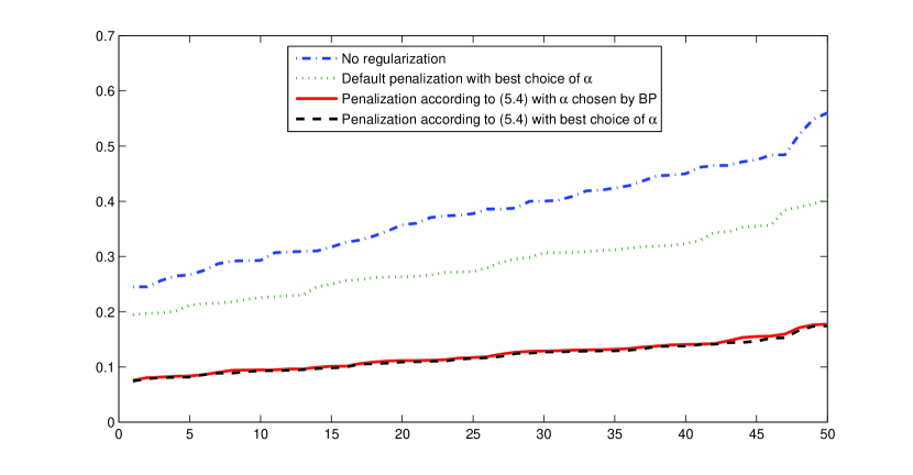
Fig. 1: Numerical illustration. The figure presents relative errors for 50 simulations of the data. The errors are plotted in ascending order for each of the discussed methods. Note that two bottom curves corresponding to penalization according to (25) nearly overlap.

To assess the obtained results and compare the performance of the considered schemes we measure the relative error

$$\frac{\left\|g-g^{\alpha,M}\right\|_{2}}{\left\|g\right\|_{2}}.$$

The results are displayed in Figure 1,where along the vertical axis we plot the relative errors in solving the problem with one of 50 simulated data. The relative errors are plotted in ascending order for each of four methods: a straightforward least-squares fit to noisy data without any regularization, the regularization with the penalization weights (25) and $\alpha$ chosen according to the balancing principle (BP) from $\Delta_{60}=\left\{\alpha_{i}=8\cdot q^{i}\ i=1,2,\ldots,60\right\},q=0.8$, the regularization with default penalization weights $\beta_{k}=1,k=0,1,\ldots,M,$ and the best $\alpha\in\Delta_{60}$, the regularization with the penalization weights (25) and the best $\alpha\in\Delta_{60}$. Thus, in the latter two cases the choice of the regularization parameter $\alpha$ for both schemes was made to achieve the best possible performance of each method. As it can be seen from Figure 1 the balancing principle (BP) performs at the level of the ideal parameter choice strategy.

From Figure 1 one can also conclude that the proper choice of the penalization weights according to the proposed a priori recipe can significantly improve the accuracy of the reconstruction. Moreover, Figure 1 shows that a straightforward least-squares fit to noisy data without regularization leads to the relative error that is about 2-3 times larger than that after a regularization. This confirms that in the considered experiment we are really dealing with a rather ill-conditioned problem.

In our second experiment we again confirm that the balancing principle gives a value of the regularization parameter $\alpha_{*}$ that is competitive with the best value manually found in [1]. We choose the regularization parameter from the same geometric sequence $\Delta_{60}$ and use the same value of the design parameter ${\omega}=0.002$ in BP.

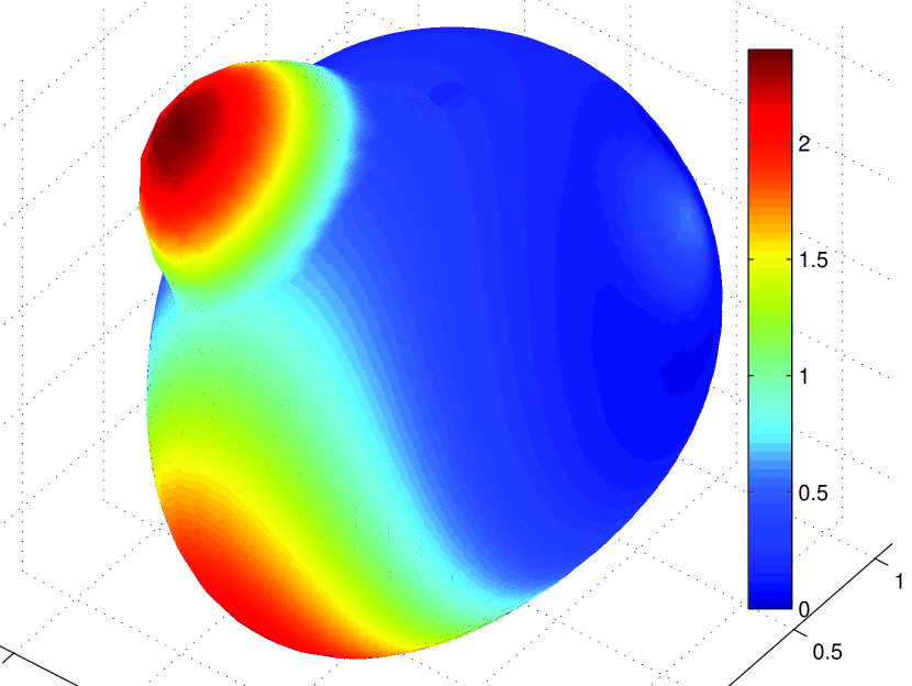
(a) $y$

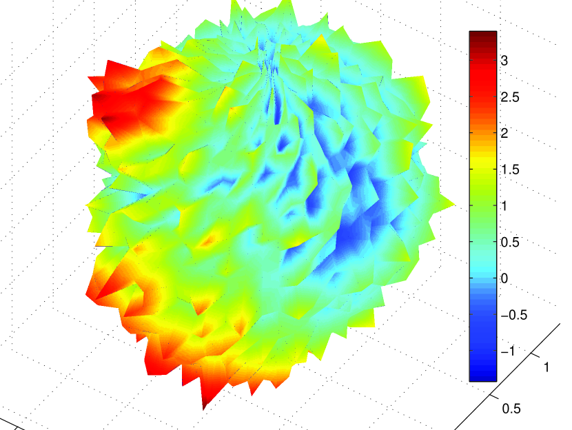
(b) $y$ with $N(0,0.25)$ noise

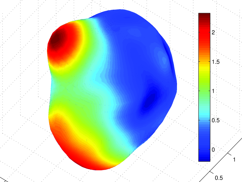
(c) $T_{\alpha_{*},M}y^{\epsilon}$

Fig. 2: Franke function recovery

Similarly to [1], as a test function $y$ we take the sum of the Franke function $y_{1}$ modified by Renka [33] (p.146) and a function $y_{\rm{cap}}$ [41], namely $y=y_{1}+y_{\rm{cap}}$ with

$$y_{1}(x_{1},x_{2},x_{3}) = 0.75e^{-(9x_{1}-2)^{2}/4-(9x_{2}-2)^{2}/4-(9x_{3}-2)^{2}/4}$$

$$+ 0.75e^{-(9x_{1}+1)^{2}/49-(9x_{2}+1)/49-(9x_{3}+1)/10}$$

$$+ 0.5e^{-(9x_{1}-7)^{2}/4-(9x_{2}-3)^{2}/4-(9x_{3}-5)^{2}/4}$$

$$- 0.2e^{-(9x_{1}-4)^{2}-(9x_{2}-7)^{2}-(9x_{3}-5)^{2}},\ (x_{1},x_{2},x_{3})\in\mathbb{S}^{2},$$

and

(31) $$y_{\rm{cap}}(\mathbf{x})=\left\{\begin{array}[]{l l}2\cos\left(\pi\arccos(\mathbf{x}_{c}\cdot\mathbf{x})\right),&\quad\mathbf{x}_{c}\cdot\mathbf{x}\geq\cos(0.5),\\ 0,&\quad\rm{otherwise},\end{array}\right.$$

where $\mathbf{x}_{c}=\left(-\frac{1}{2},-\frac{1}{2},\frac{1}{\sqrt{2}}\right)^{T}$ and $(\cdot)$ defines the dot product of two vectors. The function $y$ was then contaminated by noise, taking for the noise $\epsilon(\mathbf{x})$ at each $\mathbf{x}\in X_{N}$ an independent sample of a normal random variable with mean 0 and standard deviation $\sigma=0.5$.

Figure 2(a) illustrates the function $y$, while Figure 2(b) shows the blurred function $y^{\epsilon}(\mathbf{x})=y(\mathbf{x})+\epsilon(\mathbf{x})$.

For the reconstruction, following [1] we choose a Laplace-Beltrami penalization operator that corresponds to the matrix

$$\mathbf{B_{M}}:=\mathop{\operator@font diag}\nolimits(0,\underbrace{4,4,4}_{3},...,\underbrace{\left(M(M+1)\right)^{2},...,\left(M(M+1)\right)^{2}}_{2M+1})\in\mathbb{R}^{(M+1)^{2}\times(M+1)^{2}}.$$

Figure 2(c) illustrates the reconstructed function $T_{\alpha_{*},M}^{\beta}y^{\epsilon}$. The regularization parameter $\alpha_{*}$ was obtained according to the balancing principle described above. We found automatically the regularization parameter $\alpha_{*}=1.42\cdot 10^{-4}$ which agrees well with the value $10^{-4}$ from [1] obtained manually.

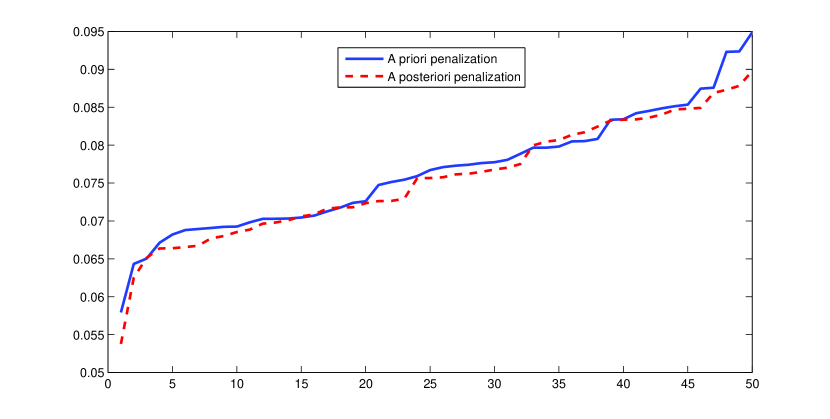
Fig. 3: Numerical illustration. The figure presents relative errors for 50 simulations of the data. The errors are plotted in ascending order for each of the discussed methods.

In our last experiment we will illustrate an application of the a posteriori rule (28) for choosing the penalization weights. As a test function $y^{\epsilon}$ we again consider the blurred function from the previous example, where we used the a priori chosen penalization weights $\beta_{k}=k(k+1)$ corresponding to Laplace-Beltrami operator. Now we are going to estimate the penalization weights using the a posteriori strategy described in Subsection 4.3.

Recall that we are looking for the minimizer (28) among the set of admissible kernels $\mathcal{K}$ consisting of the functions (29). This approach allows us to take into account an exponential, as well as a polynomial growth of $\beta_{k}$.

To find an approximate minimizer of (28) we have implemented the Random Search method [19] over the set of parameters $(\lambda_{1},\lambda_{2})\in\left[0,5\right]\times\left[0,5\right]$. The method was implemented 10 times, and in each implementation 10 random steps have been performed. Then the mean values of the parameters $\lambda_{1},\lambda_{2}$ appearing after each implementation of the Random Search method have been taken as an approximate minimum point. As the result, the values $\lambda_{1}=0.32,\lambda_{2}=1.9$ have been obtained.

Figure 3 displays the relative errors in solving the problem (6), (31) with one of 50 simulated noisy data, for each of two methods: regularization with the penalization weights $\beta_{k}=k(k+1)$, and regularization with a posteriori chosen weights.

From Figure 3 we see that the choice of the penalization weights according to the proposed a posteriori choice rule can improve the accuracy of the reconstruction.

References

- [1] C. An, X. Chen, I. H. Sloan and R. S. Womersley, Regularized least squares approximations on the sphere using spherical designs, SIAM J. Numer. Anal., 50:3 (2012), pp. 1513–1534.
- [2] N. Aronszajn, Theory of reproducing kernels, Trans. Amer. Math. Soc., 68 (1950), pp. 337–404.
- [3] E. Bannai and E. Bannai, A survey on spherical designs and algebraic combinatorics on spheres, European J. Combin., 30 (2009), pp. 1392–1425.
- [4] F. Bauer, P. Mathé and S. V. Pereverzev, Local solutions to inverse problems in geodesy. The impact of the noise covariance structure upon the accuracy of estimation, J. Geod., 81 (2007), pp. 39–51.
- [5] D. Delsarte, J. M. Goethals and J. J. Seidel, Spherical codes and designs, Geom. Dedicata, 6 (1977), pp. 363–388.
- [6] F. Filbir and W. Themistoclakis, Polynomial approximation on the sphere using scattered data, Math. Nachr., 281 (2008), pp. 650–668.
- [7] W. Freeden, Multiscale Modeling of Spaceborne Geodata, Teubner, Stuttgart, Leipzig, 1999.
- [8] W. Freeden and S. V. Pereverzev, Spherical Tikhonov regularization wavelets in satellite gravity gradiometry with random noise, J. Geod., 74 (2001), pp. 730–736.
- [9] A. Gelb, The resolution of the Gibbs phenomenon for Spherical harmonics, Math. Comput., 66:218 (1997), pp. 699–717.
- [10] M. Graf, S. Kunis and D. Potts, On the computation of nonnegative quadrature weights on the sphere, Appl. Comput. Harm. Anal., 27 (2009), pp. 124–132.
- [11] K. Hesse, I. H. Sloan and R. S. Womersley, Numerical integration on the sphere, Handbook of Geomathematics, Volume 2, Springer-Verlag Berlin Heidelberg (2010), pp. 1185–1219.
- [12] J. Keiner, S. Kunis, and D. Potts, Efficient reconstruction of functions on the sphere from scattered data, J. Fourier Anal. Appl., 13 (2007), pp. 435–458.
- [13] J. Keiner and D. Potts, Fast evaluation of quadrature formulae on the sphere, Math. Comput., 77 (2008), pp. 397–419.
- [14] Q. T. Le Gia and H. M. Mhaskar, Polynomial operators and local approximations of solutions of pseudo-differential equations on the sphere, Numer. Math., 103 (2006), pp. 299–322.
- [15] Q. T. Le Gia, H. M. Mhaskar and Q. Thong, Localized linear polynomial operators and quadrature formulas on the sphere, SIAM J. Numer. Anal., 47 (2008/09), pp. 440–466.
- [16] S. Lu and S. V. Pereverzev, Multiparameter regularization in Downward Continuation of Satellite Data , Handbook of Geomathematics, Volume 2, Springer-Verlag Berlin Heidelberg (2010), pp. 813–832.
- [17] S. Lu and S. V. Pereverzev, Regularization theory for ill-posed problems. Selected topics, Walter de Gruyter GmbH, Berlin/Boston, 2013.
- [18] P. Mathé and S. V. Pereverzev, Geometry of linear ill-posed problems in variable Hilbert scales, Inverse Problems, 19 (2003), pp. 789–803.
- [19] J. Matyas, Random optimiyation, Automat. Remote Contr., 26 (1965), pp. 244–251.
- [20] H. M. Mhaskar, On the representation of smooth functions on the sphere using finitely many bits, Appl. Comput. Harmon. Anal., 18 (2005), pp. 215–233.
- [21] H. M. Mhaskar, F. J. Narcowich, and J. D. Ward, Spherical Marcinkiewicz-Zygmund inequalities and positive quadrature, Math. Comp., 235 (2001), pp. 1113–1130.
- [22] C. A. Michelli and M. Pontil, Learning the kernel function via regularization, J. Machine Learning Res., 6 (2005), pp. 1099–1125.
- [23] C. Muller, Spherical Harmonics, Lecture notes in Math. 17, Springer-Verlag, Berlin, 1966.
- [24] F. Narcowich, P. Petrushev and J. Ward, Decomposition of Besov and Triebel-Lizorkin spaces on the sphere, J. Funct. Anal., 238 (2006), pp. 530–564.
- [25] F. Narcowich, P. Petrushev and J. Ward, Localized tight frames on spheres, SIAM J. Math. Anal., 38 (2006), pp. 574–594.
- [26] V. Naumova, S. V. Pereverzev and P. Tkachenko, Regularized collocation for Spherical harmonics Gravitational Field Modeling, Int. J. Geomath., 5 (2014), pp. 81–98.
- [27] V. Naumova, S. V. Pereverzev and S. Sivananthan, Extrapolation in variable RKHSs with application to the blood glucose reading, Inverse Problems, 27(7):075010 (2011), 13 pp.
- [28] N. K. Pavlis, S. A. Holmes, S. C. Kenyon and J. K. Factor, An earth gravitational model to degree 2160: EGM2008, EGU General Assembly, (2008), pp. 13–18.
- [29] S. V. Pereverzev and E. Schock, On the adaptive selection of the parameter in regularization of ill-posed problems, SIAM J. Numer. Anal., 43 (2005), pp. 2060–2076.
- [30] D. L. Ragozin, Constructive polynomial approximation on spheres and projective spaces, Trans. Amer. Math. Soc., 162 (1971), pp. 157–170.
- [31] M. Reimer, Multivariate polynomial approximation, International Series of Numerical Mathematics, 144, Birkhauser Verlag, Basel, 2003.
- [32] M. Reimer, Hyperinterpolation on the sphere at the minimum projection order, J. Approx. Theory, 104 (2000), pp. 272–286.
- [33] R. J. Renka, Multivariate interpolation of large sets of scattered data, ACM Trans. Math. Software, 14 (1988), pp. 139–148.
- [34] I. H. Sloan, Polynomial interpolation and hyperinterpolation over general regions, J. Approx. Theory, 83 (1995), pp. 238–254.
- [35] I. H. Sloan, Polynomial approximation on spheres – generalizing de la Vallée-Poussin, Comput. Methods Appl. Math., 11 (2011), pp. 540–552.
- [36] I. H. Sloan and R. S. Womersley, Filtered hyperinterpolation. A constructive polynomial approximation on the sphere, Int. J. Geomath., 3 (2012), pp. 95–117.
- [37] S. L. Svensson, Pseudodifferential operators – a new approach to the boundary value problems of physical geodesy, Manusc. Geod., 8 (1983), pp. 1–40.
- [38] S. L. Svensson, Solution of the altimetry-gravimetry problem, Bull. Geod., 57 (1983), pp. 332–353.
- [39] P. N. Swarztrauber, On the Spectral Approximation of Discrete Scalar and Vector Functions on a Sphere, SIAM J. Numer. Anal., 16 (1979), pp. 934–949.
- [40] G. Wahba, Spline interpolation and smoothing on the sphere, SIAM J. Sci. Statist. Comput., 2 (1981), pp. 5–16.
- [41] D. L. Williamson, J. B. Branke, J. J. Hack, R. Jakob and P. N. Swarztrauber, A standard test set for numerical approximations to the shallow water equations in spherical geometry, J. Comput. Phys., 102 (1992), pp. 211–224.
- [42] Y. Xu, Polynomial interpolation on the unit sphere, SIAM J. Numer. Anal., 41 (2003), pp. 751–766.