Creation and Amplification of Electro-Magnon Solitons by Electric Field in Nanostructured Multiferroics

Abstract

We develop a theoretical description of electro-magnon solitons in a coupled ferroelectric-ferromagnetic heterostructure. The solitons are considered in the weakly nonlinear limit as a modulation of plane waves corresponding to two, electric- and magnetic-like branches in the spectrum. Emphasis is put on magnetic-like envelope solitons that can be created by an alternating electric field. It is shown also that the magnetic pulses can be amplified by an electric field with a frequency close to the band edge of the magnetic branch.

Multiferroic materials, i.e., materials exhibiting coupled order parameters, are in the focus of current research. These systems offer not only new opportunities for applications but also provide a test ground for addressing fundamental issues regarding the interplay between electronic correlations, symmetry, and the interrelation between magnetism and ferroelectricity ME-review ; Single-ME ; Composite-ME . Here we address magnetoelectrics which possess a simultaneous ferroelectric-magnetic response. A interesting aspect is the non-linear nature of the magnetoelectric excitation dynamics, which hints at the potential of these systems for exploring nonlinear wave-localization phenomena, such as multicomponent solitons malomed1 ; malomed2 , nonlinear band-gap transmission leon ; ram1 , and the interplay between the nonlinearity and Anderson localization flach . In this paper we aim at exciting robust magnetic signals by means of electric fields. Particularly, we consider a multiferroic nano-heterostructure consisting of a ferromagnetic (FM) part deposited onto a ferroelectric (FE) substrate. As demonstrated experimentally, under favorable conditions, a coupling between the ferroelectric and the ferromagnetic order parameters may emerge (this coupling is referred to as the magnetoelectric coupling), thus allowing one to control magnetism (ferroelectricity) by means of electric (magnetic) fields. Here we consider the case when the multiferroic structure is driven by an electric field with a frequency located within the band-gap of the FE branch and in the band of the magnetic-excitation branch. For a proper choice of the electric-field frequency (that follows from the electro-magnon soliton theory developed below) it is possible to excite propagating magnetic solitons. In addition, we point out a possibility for the amplification of weak magnetic signals, which suggests the design of a digital magnetic transistor, where the role of the pump is played by the electric field.

Examples of the two-phase multiferroics under study BoRu76 ; SpFi05 ; Fi05 ; levan1 , are BaTiO₃/CoFe₂O₄ or PbZr_1-xTi_xO₃/ferrites. The developed model will be applied to a system where the FE and FM regions are coupled at an interface whith a weak magnetoelectric coupling. The theory is, however, more general and can, in principle, be applied to single-phase magnetoelectrics RaSp07 ; Dz59 ; levan2 . For the creation of electro-magnon solitons, which is the subject of the present work, a two-phase multiferroic structure is more appropriate, as it allows to generate and manipulate isolated FE or FM signals away from the interface.

Both single- and two-phase multiferroics may be modeled by a ladder consisting of two weakly coupled chains: One chain is ferroelectric (FE) built out of unidimensional electric dipole moments, $P_{n}$. The second chain is ferromagnetic (FM), composed of classical three-dimensional magnetic moments, ${\vec{S}_{n}}$, where $n$ numbers the site in the lattice. Each chain is characterized by an intrinsic nearest-neighbor coupling, and each $P_{n}$ is coupled to $\vec{S}_{n}$ via inter-chain weak magnetoelectric coupling. For a discussion of the microscopic nature of this coupling we refer to  jam . We assume the direction of FE dipoles at some arbitrary angle with respect to FM anisotropy axis $\xi$, as depicted in Fig. 1a. The magnetoelectric coupling will cause a rearrangement of magnetic moments. Let the new ground-state ordering direction of FM be the axis $z$, and $\phi$ is the angle between $z$ and anisotropy axis $\xi$. The magnetic field $\vec{h}(t)$ is applied along $z$, and $\theta$ is an angle between $z$ and FE moments (see Fig. 1a). $S_{0}$ ($P_{0}$) stands for the FM (FE) equilibrium configuration. We will consider perturbations around the equilibrium. Defining the scaled dipolar deviations $p_{n}\equiv(P_{n}-P_{0})/P_{0}$ and the scaled magnetic variables $\vec{s}_{n}\equiv\vec{S}_{n}/S_{0}$, the Hamiltonian is written as

$$H=H{{}_{\mathrm{P}}}+H{{}_{\mathrm{S}}}+H{{}_{\mathrm{SP}}},\qquad H{{}_{\mathrm{SP}}}=-\tilde{g}\sum\limits_{n=1}^{N}p_{n}s_{n}^{x},$$ (1)

$$H{{}_{\mathrm{P}}}=\sum\limits_{n=1}^{N}{\frac{\tilde{\alpha}_{0}}{2}\left(\frac{dp_{n}}{dt}\right)^{2}+\frac{\tilde{\alpha}}{2}p_{n}^{2}+\frac{\tilde{\beta}}{4}p_{n}^{4}+\frac{\tilde{\alpha}_{J}}{2}\left({p_{n+1}-p_{n}}\right)^{2}},$$

$$H{{}_{\mathrm{S}}}=\sum\limits_{n=1}^{N}\left[-\tilde{J}\vec{s}_{n}\vec{s}_{n+1}+\tilde{D}_{1}\left({s_{n}^{x}}\right)^{2}+\tilde{D}_{2}\left({s_{n}^{y}}\right)^{2}\right],$$

where $H{{}_{\mathrm{SP}}}$ stands for the linearized interfacial magnetoelectric coupling between the FM and the FE chain jam . $H{{}_{\mathrm{P}}}$ is FE part of the energy functional for $N$-interacting FE dipole moments SuJi10 ; GiChGu11 . Further, $\tilde{\alpha}_{0}$ is a kinetic coefficient; $\tilde{\alpha}_{J}$ is the nearest-neighbor coupling constant; $\tilde{\alpha}$ and $\tilde{\beta}$ are second- and forth-order expansion coefficients of the Ginzburg-Landau-Devonshire (GLD) potential RaAh07 ; SuJi10 near the equilibrium state $P_{0}$. $H{{}_{\mathrm{S}}}$ stands the ferromagnetic contribution  Ch02 , where $J$ is the nearest-neighbor exchange coupling in the FM part. $\tilde{D}_{1}=\tilde{D}S_{0}\cos^{2}\phi$ and $\tilde{D}_{2}=\tilde{D}S_{0}$ are anisotropy constants, and $D$ is the uniaxial anisotropy constant along axis $\xi$ (see Fig. 1b).

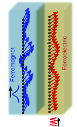
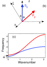
Figure 1: (Color online) (a) A schematic of the multiferroic ladder built of FE and FM chains. Arrows indicate the directions and the magnitudes of the electric dipole moments and magnetic moments in the course of the soliton advancement along the ladder. (b) Mutual orientations of FE and FM ground-state vectors, in the framework of Hamiltonian (1). (c) Dispersion relations for FE (upper) and FM (lower) branches of the multiferroic composite. The arrow indicates the selected carrier frequency.

We operate with dimensionless quantities by using the scaling $t\rightarrow\omega_{0}t$ with $\omega_{0}=\sqrt{\alpha_{J}/\alpha_{0}}$ (for the examples shown below $\omega_{0}\sim 10^{12}$ rad/sec). The other parameters of the model $\tilde{g}$, $\tilde{\alpha}$, $\tilde{\beta}$, $\tilde{J}$, $\tilde{D}_{1}$, $\tilde{D}_{2}$ are scaled with $\omega_{0}$. The scaled quantities are indicated by omitting the tilde superscript. The time evolution is governed by

$$\frac{\partial{s}_{n}^{x}}{\partial t}=-J\left[s_{n}^{y}\left(s_{n-1}^{z}+s_{n+1}^{z}\right)-s_{n}^{z}\left(s_{n-1}^{y}+s_{n+1}^{y}\right)\right]-$$

$$-2D_{2}s_{n}^{y}s_{n}^{z},$$

$$\frac{\partial{s}_{n}^{y}}{\partial t}=J\left[s_{n}^{x}\left(s_{n-1}^{z}+s_{n+1}^{z}\right)-s_{n}^{z}\left(s_{n-1}^{x}+s_{n+1}^{x}\right)\right]+$$

$$+2D_{1}s_{n}^{x}s_{n}^{z}-gp_{n}s_{n}^{z},$$ (2)

$$\frac{d^{2}p_{n}}{dt^{2}}=-\alpha p_{n}-\beta p_{n}^{3}+\left(p_{n-1}-2p_{n}+p_{n+1}\right)+gs_{n}^{x}.$$

As we are interested in small perturbations, $s_{n}^{x}$, $s_{n}^{y}$ and $p_{n}$ are much less than unity and the approximate equality $s_{n}^{z}=1-\left(s_{n}^{x}\right)^{2}/2-\left(s_{n}^{y}\right)^{2}/2$ is justified.

We seek weakly nonlinear harmonic solutions to Eq. (2), with a frequency $\omega$ and a wavenumber $k$, in the form of a column vector $\left(s_{n}^{x},s_{n}^{y},p_{n}\right)=\mathbf{R}\exp\left[i\left(\omega t-kn\right)\right]+\mathrm{c.c.}$, where $\mathbf{R}$ is a set of complex amplitudes $\mathbf{R}\equiv(a,b,c)$, and $\mathrm{c.c.}$ stands for the complex conjugate. Neglecting higher harmonics in Eq. (2), we find the set of nonlinear algebraic equations

$$\hat{\mathbf{W}}\ast\mathbf{R}=\mathbf{\emph{Q}}^{\mathrm{nl}},$$ (3)

where the matrix and source are, respectively,

$$\hat{\mathbf{W}}=\left(\begin{array}[]{ccc}i\omega&J\sin^{2}\left(k/2\right)+2D_{2}&0\\ -\left[J\sin^{2}\left(k/2\right)+2D_{2}\right]&i\omega&g\\ g&0&\omega^{2}-\alpha-\sin^{2}\left(k/2\right)\end{array}\right),$$

$$\textbf{\emph{Q}}^{nl}=\left(\begin{array}[]{c}b(|b|^{2}+|a|^{2})(J-J\cos k+D_{2})-b^{*}(b^{2}+a^{2})(J\cos k-J\cos 2k-D_{2})\\ -a(|b|^{2}+|a|^{2})(J-J\cos k+D_{1})+a^{*}(b^{2}+a^{2})(J\cos k-J\cos 2k-D_{1})\\ -3\beta|c|^{2}c\\ \end{array}\right).$$ (7)

The linear limit amounts to the set of linear homogeneous algebraic equations $\hat{\mathbf{W}}\ast\mathbf{R}=0$. The solvability condition $\mathrm{Det}\left(\hat{\mathbf{W}}\right)=0$ leads to two branches of the dispersion relation $\omega(k)$ which are shown in Fig. 1(c), with the corresponding amplitude set, $\mathbf{R}=(a,b,c)$, where $b$ and $c$ are expressed via the arbitrary constant $a$: $b=-ia\omega/\left[J\sin^{2}(k/2)+D_{2}\right]$, $c=ga/\left[\alpha+\sin^{2}(k/2)-\omega\right]$. We call a dispersion branch ferroelectric (defining its frequency $\omega_{E}$ and labeling the amplitude with index $E$), if it has $|c|>|a|$ [the red curve in Fig. 1(c)], while a ferromagnetic branch ($\omega_{M}$) is defined by the relation $|c|<|a|$ (the blue curve in the same figure).

Of a particular interest is the case when the system is excited at an edge (at the left one, for the sake of definiteness), with a frequency $\omega_{s}$ which falls into the bandgap of FE mode and, simultaneously, the propagation band of the FM one, as shown by the arrow in Fig. 1(c). The dispersion relation with the fixed frequency, $\omega=\omega_{s}$ becomes then a cubic equation for $\sin^{2}(k/2)$. For $\omega_{s}$ belonging to the band of FM mode and bandgap of FE one, the cubic equation yields two complex wavenumbers, associated with FE and FM modes, and a real one, corresponding to the FM mode. These three wavenumbers determine a set of three orthogonal eigenvectors, $\mathbf{R_{E}}\equiv(a_{E},b_{E},c_{E})$, $\mathbf{R_{M}^{-}}\equiv(a_{M}^{-},b_{M}^{-},c_{M}^{-})$ and $\mathbf{R_{M}^{+}\equiv(a_{M}^{+},b_{M}^{+},c_{M}^{+})}$, where the first two correspond to complex FE and FM wavenumbers, $k_{E}$ and $k_{M}^{-}$, respectively, while the last one is related to the real wavenumber, $k_{M}^{+}$. In linear systems, the solutions with the complex wavenumbers are evanescent waves localized at the left edge of the multiferroic chain. Thus, the solution for the vector function, $\mathbf{F_{n}}=\left(s_{n}^{x},s_{n}^{y},p_{n}\right)$, is

$$\mathbf{F_{n}^{E}} = A(t)\mathbf{R_{E}}e^{i\omega_{s}t-|k_{E}|n}+c.c.$$

$$\mathbf{F_{n}^{M^{-}}} = B(t)\mathbf{R_{M}^{-}}e^{i\omega_{s}t-|k_{M}^{-}|n}+c.c.$$ (8)

where the amplitudes $A(t)$ and $B(t)$ may vary slowly in time.

As mentioned above, the solutions corresponding to the complex wavenumbers are localized at the boundary. To examine the possibility of a solitonic self-localization of the third solution with a real wavenumber (cf. Refs. new ; kalinikos ; ram for similar solutions in multiferroic models), we consider the nonlinear frequency shift produced by the small terms $\mathbf{\emph{Q}}^{\mathrm{nl}}$ in (3). Assuming a shifted frequency, $\omega+\delta\omega$ instead of $\omega$, the matrix $\hat{\mathbf{W}}$ is substituted by a modified one, $\hat{\mathbf{W}}+\mathbf{\delta\hat{W}}$, with the diagonal matrix $\mathbf{\delta\hat{W}}\equiv i\delta\omega\cdot\mathrm{Diag}(1,1,2\omega)$. We also define a row vector $\mathbf{L}=(a^{\prime},b^{\prime},c^{\prime})$ which solves for the equation $\mathbf{L}\ast\hat{\mathbf{W}}=0$. Then, multiplying both sides of Eq. (3) on $\mathbf{L}$, we obtain the nonlinear plane-wave frequency shift:

$$\delta\omega\left(k,|a|^{2}\right)=-i\left(\mathbf{L}\ast\mathbf{\emph{Q}}^{\mathrm{nl}}\right)\biggr{/}\left(\mathbf{L}\ast\mathbf{\delta\hat{W}\ast R}\right).$$ (9)

From these results, operating with the envelope function $\varphi(n,t)$ defined from $\mathbf{F_{n}^{M^{+}}}=\varphi(n,t)e^{i\left(\omega_{s}t-ik_{M}^{+}n\right)}\left(a_{M}^{+},~{}b_{M}^{+},~{}c_{M}^{+}\right)$, one can derive the nonlinear Schrödinger equation (NLS), cf. Refs. boardman ; taniuti in the form:

$$2i\left(\frac{\partial\varphi}{\partial t}+v\frac{\partial\varphi}{\partial n}\right)+\omega^{\prime\prime}\frac{\partial^{2}\varphi}{\partial n^{2}}+\Delta|\varphi|^{2}\varphi=0,$$ (10)

which gives rise to the respective envelope-soliton solution with the FM-like localized mode being written as

$$\mathbf{F_{n}^{M^{+}}}=\frac{e^{i\left(\omega_{s}t-k_{M}^{+}n\right)}}{{\cosh}\left[\frac{a_{M}^{+}}{2}\sqrt{\frac{\Delta}{2\omega^{\prime\prime}}}(n-vt)\right]}\left(\begin{array}[]{c}a_{M}^{+}\\ b_{M}^{+}\\ c_{M}^{+}\\ \end{array}\right)\mathrm{+c.c.}.$$ (11)

The velocity, dispersion, and the nonlinearity coefficients are

$$v=\frac{\partial\omega_{M}}{\partial k},\quad\omega^{\prime\prime}=-\frac{\partial^{2}\omega_{M}}{\partial k^{2}},\quad\Delta=\frac{\partial\left[\delta\omega_{M}(k,|a|^{2})\right]}{\partial\left[|a|^{2}\right]}.$$ (12)

The carrier frequency of this soliton is defined by the dispersion relation [the lower blue curve in Fig. 1(c)]:

$$\omega_{s}=\omega_{M}(k)+\delta\omega_{M}\left(k,|a|^{2}\right)/2.$$ (13)

Thus, one can generate both the FE evanescent (8) and FM solitonic (11) modes, driving the left edge of the chain at the same frequency, $\omega_{s}$. It is possible to produce a combination of these solutions too. Generally in nonlinear systems, linear combinations of particular solutions is not another solution but if the solutions are far separated, which makes interactions between them negligible, the linear combination

$$\mathbf{F_{n}}=f_{1}\mathbf{F_{n}^{E}}+f_{2}\mathbf{F_{n}^{M^{-}}}+\mathbf{F_{n}^{M^{+}}}$$ (14)

is still a solution of the nonlinear problem. In the weakly nonlinear limit it is even possible to construct a solution for the case when particular modes overlap (i.e., the magnetic soliton is located near the edge), adding a time-dependent phase to each term (8) and (11) in the sum oikawa . For instance, one can consider an approximate solution at the left edge of the ladder, $n=0$, in the form of

$$\mathbf{F_{0}}=f_{1}\mathbf{F_{0}^{E}}e^{i\Psi^{E}(t)}+f_{2}\mathbf{F_{0}^{M^{-}}}e^{i\Psi^{M^{-}}(t)}+\mathbf{F_{0}^{M^{+}}}e^{i\Psi^{M^{+}}(t)},$$ (15)

where, in the weakly-nonlinear limit, the phases $\Psi$ are proportional to the wave amplitudes. Hence the waves do not gain significant phase shifts due to interaction effects, if their relative group velocity is not negligible. In this case, all phase shifts may be neglected.

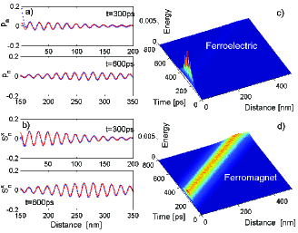
Figure 2: (Color online) Numerical simulations of the creation of a ferromagnetic soliton by the electric field, using Eq. (2) with parameters (19). (a,b) Show a comparison between the analytical (solid lines) and the numerical (points) results for the soliton’s spatial profile at different moments of time. The analytical solution is taken according to Eq. (14) with the coefficients (18). (c,d): The propagation of the FM soliton in the ferroelectric and the ferromagnetic layers, respectively.

Our particular aim is to create an FM soliton by exciting only the FE degree of freedom at the edge, i.e., $s_{0}^{x}=s_{0}^{y}=0$. To this end, we choose $A(t)=B(t)=\mathrm{sech}\left[a_{M}^{+}vt\sqrt{\Delta\Bigr{/}8\omega^{\prime\prime}}\right]$, seeking to impose the following vector relation at the edge, $n=0$:

$$(0,0,p_{0})=\frac{\left(f_{1}\mathbf{R_{E}}+f_{2}\mathbf{R_{M}^{-}}+\mathbf{R_{M}^{+}}\right)e^{i\omega_{s}t}}{\cosh\left[a_{M}^{+}vt\sqrt{\Delta/8\omega^{\prime\prime}}\right]}+\mathrm{c.c.}$$ (16)

Using now the orthogonality of eigenvectors $\mathbf{R}$, we readily get the appropriate expression for $p_{0}$:

$$p_{0}(t)=\frac{\Bigl{|}\mathbf{R_{M}^{+}}\Bigr{|}^{2}}{\left(c_{M}^{+}\right)^{\ast}}\frac{e^{i\omega_{s}t}}{\cosh\left[a_{M}^{+}vt\sqrt{\Delta/8\omega^{\prime\prime}}\right]}+\mathrm{c.c.}$$ (17)

Further, it is possible to compute the coefficients $f_{1}$ and $f_{2}$, using the same orthogonality property:

$$f_{1}=\frac{\left|\mathbf{R_{M}^{+}}\right|^{2}\left(c_{E}\right)^{\ast}}{\left|\mathbf{R_{E}}\right|^{2}\left(c_{M}^{+}\right)^{\ast}};\quad f_{2}=\frac{\left|\mathbf{R_{M}^{+}}\right|^{2}\left(c_{M}^{-}\right)^{\ast}}{\left|\mathbf{R_{M}^{-}}\right|^{2}\left(c_{M}^{+}\right)^{\ast}}.$$ (18)

In numerical simulations, if we make $p_{0}$ a function of time as per Eq. (17), keeping the magnetic moments pinned at the boundary, it is possible to excite the FE and FM evanescent waves (8), and also propagating FM soliton (11). These simulations correspond to an experimental setup with pinned boundary conditions at both FE and FM edges, and to the application of the electric field $E(t)=p_{0}(t)$ according to Eq. (17) at the first cell of the FE chain. In this way, one can realize the excitation of magnetic solitons in the FM chain of the multiferroic ladder via an electric (rather than magnetic) field by virtue of the magnetoelectric coupling.

For an assessment of the above, we performed full numerical simulations with the following values of the normalized parameters

$$\alpha=0.2;~{}\beta=0.1;~{}J=1;~{}D_{1}=0.1;~{}D_{2}=0.2;~{}g=0.1.$$ (19)

These values correspond to $BaTiO_{3}/Fe$ DuJa06 ; LeSa10 . Furthermore, we assume for the FE second and fourth order potential coefficients $\tilde{\alpha}_{1}/(a^{3}_{\mathrm{FE}})=2.77\cdot 10^{7}$ [Vm/C], $\tilde{\alpha}_{2}/(a^{3}_{\mathrm{FE}})=1.7\cdot 10^{8}$ [Vm⁵/C³], and for the FE coupling coefficient $\tilde{\alpha}_{J}/(a^{3}_{\mathrm{FE}})=1.3\cdot 10^{8}$ [Vm/C], the equilibrium polarization $P_{0}=0.265$ [C/m²], and the coarse-grained FE cell size $a_{\mathrm{FE}}=1$ [nm]. The FM exchange interaction strength is $\tilde{J}=3.15\cdot 10^{-20}$ [J], the FM anisotropy constant is $\tilde{D}=6.75\cdot 10^{-21}$ [J], and the ME coupling strength is $\tilde{g}_{0}\approx 10^{-21}$ [Vm²].

We drive the left boundary of FE according to (17) with a driving frequency $\omega_{s}=0.4$ and an amplitude $a_{M}^{+}=0.07$ and apply pinned boundary conditions for FM, $s_{0}^{x}=s_{0}^{y}=0$. The results are displayed in Fig. 2, where the comparison of numerical simulations and approximate analytical solution (14) are shown at different moments of time [Figs. 2(a,b)].

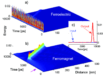
Figure 3: (Color online) Results of numerical simulations of the amplification of a magnetic signal in the multiferroic chain (a). The space-time evolution of excitations in the ferroelectric part. (b) The amplified propagation of the magnetic soliton in the ferromagnetic part. The arrow indicates the moment of the injection of the magnetic signal. Inset (c) presents the time dependence of the energy of the input magnetic signal at the FM edge, $n=0$, while the energy of output signal is measured at site $n=200$.

Next, let us envisage the possibility of amplifying magnetic pulses: We apply a continuous electric signal with the frequency $\omega_{s}$ which is slightly below the FM band boundary, $\omega_{M}(0)$, keeping FM moments pinned at the edge. In this setting, and for small driving amplitudes, no energy is transmitted through the chain. Both FM and FE modes are evanescent and described by the solutions (8). A propagating FM soliton emerges only if the electric-field amplitude attains the band gap transmission threshold leon ; rk : This happens if the amplitude is large enough so that a solution of the nonlinear dispersion relation (13) for real wave number $k$ exits. Then, if one keeps the amplitude of the electric field just slightly below this band gap threshold, a small-amplitude in-phase magnetic signal coupled to FM chain allows to pass the threshold. This gives rise to a large-amplitude FM soliton propagating through the multiferroic, see Fig. 3. In this way, one can realize an amplification of the magnetic pulses by electric field. It may happen that almost all the energy of the electric field will be transferred to the ferromagnet chain, and the corresponding amplification rate may achieve values as much as $\sim 100$. For instance, in the simulations presented in Fig. 3 we choose the driving frequency and the amplitude of the electric field $\omega_{s}=0.229$ (that is $\approx 30$ GHz in real units) and $\left(p_{0}\right)_{\max}=0.414$, while the FM signal amplitude is $\left(s_{0}^{x}\right)_{max}=0.02$.

In this paper we do not address dissipation effects which, in principle, could be taken into account by introducing the conventional Landau-Lifshitz-Gilbert damping term in the magnetic part of the evolution equations (2), as well as damping terms in the electric part. Here, we assume that dissipation has no qualitative effects for the considered length and on the time scales comparable with magnetic/electric signal transmission (that is $10^{-9}$sec) and do not consider thus the respective terms in the evolution equations.

Concluding, an electro-magnon soliton theory is developed and the results are applied for electric field-induced magnetic soliton generation. A proper choice of pump electric field parameters enables an amplification of magnetic signals. In the amplifying regime the total (pump+signal) amplitude overcomes the band-gap transmission threshold and the energy of electric field is completely transferred to the magnetic soliton. As we have shown above, substantial (more than $100$ times) amplification of the magnetic input/output signals could be realized.

Acknowledgements.- L.Ch. and J.B. are supported by DFG through SFB 762. R.Kh. is supported by DAAD fellowship and grant No 30/12 from SRNSF. The work of B.A.M. was supported, in part, by the German-Israel Foundation through grant No. I-1024-2.7/2009.

References

- (1) W. Eerenstein, N. D. Mathur, and J. F. Scott, Nature 442, 759 (2006).
- (2) Y. Tokura and S. Seki, Adv. Mater. 22, 1554 (2010).
- (3) C. A. F. Vaz, J. Hoffman, Ch. H. Ahn, and R. Ramesh, Adv. Mater. 22, 2900 (2010).
- (4) D.J. Kaup and B.A. Malomed, J. Opt. Soc. Am. B, 15, 2838, (1998).
- (5) V.S. Shchesnovich, B.A. Malomed, R.A. Kraenkel, Physica D, 188, 213 (2004).
- (6) F. Geniet and J. Leon, Phys. Rev. Lett. 89, 134102 (2002).
- (7) R. Khomeriki, Phys. Rev. Lett., 92, 063905 (2004).
- (8) S. Flach, D. O. Krimer, and Ch. Skokos Phys. Rev. Lett. 102, 024101 (2009).
- (9) J. van den Boomgaard, A. M. J. G. van Run, and J. van Suchtelen, Ferroelectrics 10, 295 (1976).
- (10) N. Spaldin and M. Fiebig, Science 309, 391 (2005).
- (11) M. Fiebig, J. Phys. D: Appl. Phys. 38, R123 (2005).
- (12) Sukhov A., Chotorlishvili L., Horley P.P., Jia C.-L., Mishra S., and Berakdar J. J. Phys. D: Appl. Phys. 47, 155302 (2014).
- (13) R. Ramesh and N. A. Spaldin, Nat. Mater. 6, 21 (2007).
- (14) I. E. Dzyaloshinkskii, Sov. Phys. JETP 10, 628 (1959).
- (15) Azimi M., Chotorlishvili L., Mishra S. K., Greschner S., Vekua T., and Berakdar J. Phys. Rev. B 89, 024424 (2014); Azimi M., Chotorlishvili L., Mishra S. K., Vekua T., Hbner W. and Berakdar J.New Journal of Physics 16, 063018 (2014).
- (16) C.-L. Jia, T.-L. Wei, C.-J. Jiang, D.-S. Xue, A. Sukhov, and J. Berakdar, Phys. Rev. B, 90, 054423 (2014).
- (17) A. Sukhov, C.-L. Jia, P. P. Horley, and J. Berakdar, J. Phys.: Cond. Matt. 22, 352201 (2010); Phys. Rev. B 85, 054401 (2012); EPL 99, 17004 (2012); Ferroelectrics 428, 109 (2012); J. Appl. Phys. 113, 013908 (2013); Phys. Rev. B. 90, 224428 (2014).
- (18) P. Giri, K. Choudhary, A. S. Gupta, A. K. Bandyopadhyay, and A. R. McGurn, Phys. Rev. B 84, 155429 (2011).
- (19) Physics of Ferroelectrics, K. Rabe, Ch. H. Ahn and J.-M. Triscone (Eds.), (Springer, Berlin 2007).
- (20) Physics of Ferromagnetism, S. Chikazumi, (Oxford University Press Inc., New York 2002).
- (21) F. Kh. Abdullaev, A. A. Abdumalikov, and B. A. Umarov, Phys. Lett. A 171, 125-128 (1992).
- (22) M.A. Cherkasskii, B.A. Kalinikos, JETP Lett., 97, 611, (2013).
- (23) L. Chotorlishvili, R. Khomeriki, A. Sukhov, S. Ruffo, and J. Berakdar, Phys. Rev. Lett. 111, 117202 (2013).
- (24) J. W. Boyle, S. A. Nikitov, A. D. Boardman, J. G. Booth, and K. Booth, Phys. Rev. B, 53, 12173 (1996).
- (25) T. Taniuti and N. Yajima, J. Math. Phys., 10, 1369, (1969).
- (26) M. Oikawa and N. Yajima, J. Phys., Soc. Jpn., 37, 486 (1974).
- (27) C.-G. Duan, S. S. Jaswal, and E. Y. Tsymbal, Phys. Rev. Lett. 97, 047201 (2006).
- (28) J.-W. Lee, N. Sai, T. Cai, Q. Niu, A.A. Demkov, Phys. Rev. B 81, 144425 (2010).
- (29) R. Khomeriki and D. Chevriaux, J. Leon, Eur. Phys. J. B, 49, 213 (2006).