Impact of Baryonic Processes on Weak Lensing Cosmology:
Power Spectrum, Non-Local Statistics, and Parameter Bias

Abstract

We study the impact of baryonic physics on cosmological parameter estimation with weak lensing surveys. We run a set of cosmological hydrodynamics simulations with different galaxy formation models. We then perform ray-tracing simulations through the total matter density field to generate 100 independent convergence maps of 25 ${\rm deg}^{2}$ field-of-view, and use them to examine the ability of the following three lensing statistics as cosmological probes; power spectrum, peak counts, and Minkowski functionals. For the upcoming wide-field observations such as Subaru Hyper Suprime-Cam (HSC) survey with a sky coverage of 1400 ${\rm deg}^{2}$, these three statistics provide tight constraints on the matter density, density fluctuation amplitude, and dark energy equation of state, but parameter bias is induced by the baryonic processes such as gas cooling and stellar feedback. When we use power spectrum, peak counts, and Minkowski functionals, the magnitude of relative bias in the dark energy equation of state parameter $w$ is at a level of, respectively, $\delta w\sim 0.017$, $0.061$, and $0.0011$. For HSC survey, these values are smaller than the statistical errors estimated from Fisher analysis. The bias can be significant when the statistical errors become small in future observations with a much larger survey area. We find the bias is induced in different directions in the parameter space depending on the statistics employed. While the two-point statistic, i.e. power spectrum, yields robust results against baryonic effects, the overall constraining power is weak compared with peak counts and Minkowski functionals. On the other hand, using one of peak counts or Minkowski functionals, or combined analysis with multiple statistics, results in biased parameter estimate. The bias can be as large as $1\sigma$ for HSC survey, and will be more significant for upcoming wider area surveys. We suggest to use an optimized combination so that the baryonic effects on parameter estimation are mitigated. Such ‘calibrated’ combination can place stringent and robust constraints on cosmological parameters.

1. INTRODUCTION

An array of recent observations of the large-scale structure of the universe such as cosmic microwave background (CMB) anisotropies (e.g., Hinshaw et al., 2013; Planck Collaboration et al., 2014) and galaxy clustering (e.g., Reid et al., 2010; Beutler et al., 2014) established the standard cosmological model called $\Lambda$CDM model. In $\Lambda$CDM model, the energy content of the present-day universe is dominated by two mysterious components: dark energy and dark matter. Dark energy realizes the cosmic acceleration at present and dark matter plays an important role of formation of rich structure in the universe. However, we have not understood yet the nature of dark energy and the physical properties of dark matter. In order to reveal the mysterious dark components in the universe, several observational programs are proposed and still under investigation. Such observational programs include Subaru Hyper Suprime-Cam (HSC), the Dark Energy Survey (DES), and the Large Synoptic Survey Telescope (LSST). Space missions such as Euclid and WFIRST are also promising. Gravitational lensing is expected to be the main subject of these future surveys that are aimed at studying the large-scale structure of the universe at present and in the past.

Weak gravitational lensing (WL) by large-scale structure in the universe is the promising probe into properties of dark matter and dark energy (for a review, see Bartelmann & Schneider, 2001; Munshi et al., 2008; Kilbinger, 2014). WL causes small distortion of image of distant source galaxies, called cosmic shear, which reflect directly the intervening matter distribution along a line of sight. Recent cosmic shear observations have proved WL measurement to be a powerful tool for studying dark matter distribution in the universe, from which one can extract information on the basic cosmological parameters (e.g., Massey et al. (2007); Kilbinger et al. (2013)). Forthcoming weak-lensing surveys are aimed at measuring cosmic shear over a wide area of more than 1000 ${\rm deg}^{2}$. These observations will address important questions of dark matter and dark energy at unprecedented precision.

Unfortunately, major statistical methods to make the best use of WL data in upcoming surveys are still under debate. The problem originates from the fact that cosmic shear follows non-Gaussian probability distribution due to non-linear gravitational growth (Sato et al., 2009). In order to incorporate the non-linear features accurately into WL statistics, cosmological $N$-body simulations have been extensively used. Previous numerical studies (Hilbert et al., 2009; Sato et al., 2009, 2011) have already provided important guides for cosmological studies with WL statistics. There still remain several possible factors to be examined. One of the uncertainties in such studies is the effects of baryonic physics. Modeling baryonic effects on the WL statistics is difficult because of the overall complexities in galaxy formation. Recent numerical simulations and semi-analytic methods successfully reproduce key observational data (Duffy et al., 2010; Martizzi et al., 2012; Schaye et al., 2014; Okamoto et al., 2014; Martizzi et al., 2014; Schaller et al., 2014a, b; Velliscig et al., 2014; Pike et al., 2014). Some of these studies focus on active galactic nuclei (AGN) feedback, which quenches star formation in massive halos and may solve over cooling problem (i.e. the over production of stars in numerical simulations). These simulations also show that baryonic physics can change significantly the distribution of both dark matter and baryons within a halo. However, since baryonic effects are expected to be weak at large scale, most of WL studies so far are based on simulations with dark matter component only. For future ‘precision cosmology’ with WL, neglecting various astrophysical processes may lead to undesirable bias of cosmological parameter estimation, as has been pointed out by several studies (Jing et al., 2006; Semboloni et al., 2011; Zentner et al., 2013; Yang et al., 2013; Mohammed et al., 2014). Hence, it is crucial and timely to study the effects of baryonic physics on WL statistics in detail.

In this paper, we use several statistics to extract the non-Gaussian information of WL maps. In addition to power spectrum (PS) of weak lensing convergence, we consider peak counts and the Minkowski Functionals (MFs). Kratochvil et al. (2010) show that peak counts on lensing map can be indeed useful for cosmological parameter estimation. High-$\sigma$ lensing peaks are likely associated with massive dark matter halos along a line of sight (Hamana et al., 2004; Yang et al., 2011; Hamana et al., 2012). MFs are morphological statistics for a given multi-dimensional field. MFs are one of the good measure of topology in WL and contain the suitable cosmological information beyond two-point statistics (Munshi et al., 2012; Kratochvil et al., 2012; Shirasaki et al., 2012; Shirasaki & Yoshida, 2014). Throughout this paper, we use the terms “local statistics” and “non-local statistics”. Shear two-point correlation functions and the corresponding power spectrum are measured directly from shear that is obtained from local measurements, i.e., from galaxy ellipticities. Peak counts and MFs are non-local statistics, because they can be obtained from convergence maps that are derived by integrating shear over the region of interest. In order to clarify the baryonic effects on the WL statistics, we utilize a large set of hydrodynamical $N$-body simulations including various baryonic processes. We then study how the baryonic effects bias cosmological parameter estimation with WL measurement. The rest of this paper is organized as follows. In Section 2, we summarize the basics of WL statistics of interest and the implementations to estimate the statistics for a given WL data. In Section 3, we describe our simulation set that includes cosmological simulations with baryonic physics. In Section 4, we provide the details of analysis performed in this paper. In Section 5, we show the impact of baryonic physics on WL statistics. We also perform a Fisher analysis to present the expected cosmological constraints in upcoming lensing surveys. We show the results of $\chi^{2}$ analysis to quantify the baryonic effects on parameter estimation with WL statistics. Concluding remarks and discussions are given in Section 6.

2. WEAK LENSING STATISTICS

We first summarize the basics of gravitational lensing by large-scale structure. Weak gravitational lensing effect is characterized by the image distortion of a source object by the following 2D matrix:

$$A_{ij}=\frac{\partial\beta^{i}}{\partial\theta^{j}}\equiv\left(\begin{array}[]{cc}1-\kappa-\gamma_{1}&-\gamma_{2}\\ -\gamma_{2}&1-\kappa+\gamma_{1}\\ \end{array}\right),$$ (3)

where the observed position of a source object is denoted by $\theta$, the true position is $\beta$, $\kappa$ is convergence, and $\gamma$ is shear. In weak field, where gravitational potential is small compared with $c^{2}$, each component of $A_{ij}$ can be related to the second derivative of the gravitational potential $\Phi$ as

$$A_{ij} = \delta_{ij}-\Phi_{ij},$$ (4)

$$\Phi_{ij} = \frac{2}{c^{2}}\int_{0}^{\chi}{\rm d}\chi^{\prime}f(\chi,\chi^{\prime})\frac{\partial^{2}}{\partial x_{i}\partial x_{j}}\Phi[r(\chi^{\prime})\mbox{\boldmath$\theta$},\chi^{\prime}],$$ (5)

$$f(\chi,\chi^{\prime}) = \frac{r(\chi-\chi^{\prime})r(\chi^{\prime})}{r(\chi)},$$ (6)

where $r(\chi)$ is angular diameter distance, and $x_{i}=r\theta_{i}$ represents physical separation (Bartelmann & Schneider, 2001; Munshi et al., 2008). By using the Poisson equation and Born approximation (Bartelmann & Schneider, 2001; Munshi et al., 2008), one can express weak lensing convergence field as

$$\kappa(\mbox{\boldmath$\theta$},\chi)=\frac{3}{2}\left(\frac{H_{0}}{c}\right)^{2}\Omega_{\rm m}\int_{0}^{\chi}{\rm d}\chi^{\prime}f(\chi,\chi^{\prime})\frac{\delta[r(\chi^{\prime})\mbox{\boldmath$\theta$},\chi^{\prime}]}{a(\chi^{\prime})}.$$ (7)

Born approximation yields sufficiently accurate two-point statistics (e.g., Schneider et al., 1998). In the present paper, we take into account the non-linearity of convergence shown in Eq. (5) by performing ray-tracing simulations through the matter density field obtained from cosmological simulations.

2.1. Observables

Here, we summarize three different statistics of weak lensing convergence field, power spectrum (PS), peak counts, and Minkowski Functionals (MFs). PS has complete cosmological information only if statistical properties of matter fluctuation follows Gaussian distribution. However, non-linear structure formation induced by gravity inevitably makes the fluctuation deviate significantly from Gaussian. In order to extract cosmological information, we will also use non-local statistics, i.e. peak counts and MFs.

2.1.1 Power spectrum

PS is one of the basic statistics for modern cosmology. For a convergence field $\kappa$, PS is defined by the two point correlation in Fourier space:

$$\langle\tilde{\kappa}(\bm{\ell})\tilde{\kappa}^{*}(\bm{\ell}^{\prime})\rangle=(2\pi)^{2}\delta_{D}(\bm{\ell}-\bm{\ell}^{\prime})P_{\kappa}(\ell),$$ (8)

where the multipole $\ell$ is related with angular scale through $\theta=\pi/\ell$. By using Limber approximation (Limber, 1954; Kaiser, 1992) and Eq. (7), one can derive the convergence power spectrum as

$$P_{\kappa}(\ell) = \int_{0}^{\chi_{s}}{\rm d}\chi\frac{W(\chi)^{2}}{r(\chi)^{2}}P_{\delta}\left(k=\frac{\ell}{r(\chi)},z(\chi)\right),$$ (9)

where $P_{\delta}(k)$ represents the three dimensional matter power spectrum, $\chi_{s}$ is comoving distance to source galaxies and $W(\chi)$ is the lensing weight function defined as

$$W(\chi)=\frac{3}{2}\left(\frac{H_{0}}{c}\right)^{2}\Omega_{\rm m}\frac{r(\chi_{s}-\chi)r(\chi)}{r(\chi_{s})}(1+z(\chi)).$$ (10)

We follow Sato et al. (2009) to estimate the convergence PS from numerical simulations. We measure the binned power spectrum of convergence field by averaging the product of Fourier modes $|\tilde{\kappa}(\mbox{\boldmath$\ell$})|^{2}$. We use 20 bins logarithmically spaced in the range of $\ell=100$ to $10^{5}$. For parameter estimation performed in section 4, we re-compute PS using 10 bins logarithmically spaced in the range of $\ell=100$ to $2000$.

2.1.2 Peak count

Peaks in convergence maps can be a probe of massive halos (Hamana et al., 2004, 2012) and thus contain cosmological information (Yang et al., 2011).

In practice, peaks on convergence map is defined by a local maxima on the “smoothed” map. We do the map-smoothing because the observed lensing field is significantly contaminated by the intrinsic ellipticities of source galaxies. The contaminant is called shape noise, which is indeed the major contribution to the measured shape of source galaxies. In practice, we use a Gaussian window function in order to reduce the effect of shape noises on WL statistics. The smoothed convergence $\mathcal{K}(\bm{\theta};\theta_{G})$ can be written as convolution with a filter function of $W_{G}$:

$$\mathcal{K}(\bm{\theta};\theta_{G})=\int{\rm d}^{2}\phi\ W_{G}(\bm{\theta}-\bm{\phi};\theta_{G})\kappa(\bm{\phi}),$$ (11)

where $\theta_{G}$ is the smoothing scale and $W_{G}$ is a gaussian filter given by

$$W_{G}(\bm{\theta})=\frac{1}{\pi\theta_{G}^{2}}\exp\left(-\frac{\theta_{1}^{2}+\theta_{2}^{2}}{\theta_{G}^{2}}\right).$$ (12)

One can evaluate the smoothed convergence due to an isolated massive cluster at a given redshift by assuming the universal matter density profile of dark matter halos (e.g., Navarro et al., 1997b). A simple theoretical framework to predict the number density of the $\mathcal{K}$ peaks is presented by Hamana et al. (2004); Maturi et al. (2011). Their calculation yields reasonable results when the signal-to-noise ratio of $\mathcal{K}$ due to massive halos is larger than $\sim 4$ (see, Hamana et al., 2004, for details). Fan et al. (2010) also consider more detailed calculation by including the statistical properties of shape noise and the impact of shape noise on peak position.

In order to locate peaks on a discretized map obtained from numerical simulations, we define the peak as a pixel that is higher than eight neighboring pixels. We then measure the number density of peaks as a function of $\mathcal{K}$. We exclude the region within 2$\theta_{G}$ from the boundary of the map in order to avoid the effect of incomplete smoothing. In this paper, we divide peaks into two subgroups: “medium peaks (MPs)” and “high peaks (HPs)”. We define MPs and HPs by the peak height in a similar manner to Yang et al. (2013). The former is defined by the covergence peak with $1.0\leq\mathcal{K}_{\mathrm{peak}}/\sigma_{\mathrm{noise}}\leq 3.0$ whereas the latter corresponds to the peak with $3.0\leq\mathcal{K}_{\mathrm{peak}}/\sigma_{\mathrm{noise}}\leq 5.0$. Here, $\sigma_{\mathrm{noise}}$ is the rms of shape noise on smoothed map given by Eq. (25). It is important to note that these peaks are thought to have different physical origins. MPs are likely caused by the shape noise or/and several dark matter halos aligned along a line of sight (Yang et al., 2011), whereas HPs are associated with individual massive dark matter halos (e.g., Hamana et al., 2004). Throughout the paper, we set the number of bins to be 10 for parameter estimation when measuring peak count of each subgroup.

2.1.3 Minkowski Functionals

MFs are morphological descriptors for smoothed random fields. There are three kinds of MFs for two-dimensional maps. Each MFs of $V_{0}$, $V_{1}$, and $V_{2}$ represent the area above the threshold $\nu$, the total boundary length, the integral of geodesic curvature along the contours. They are given by

$$V_{0}(\nu) \equiv \frac{1}{A}\int_{Q_{\nu}}{\rm d}a,$$ (13)

$$V_{1}(\nu) \equiv \frac{1}{A}\int_{\partial Q_{\nu}}\frac{1}{4}{\rm d}\ell,$$ (14)

$$V_{2}(\nu) \equiv \frac{1}{A}\int_{\partial Q_{\nu}}\frac{1}{2\pi}K{\rm d}\ell,$$ (15)

where $K$ is the geodesic curvature of the contours, ${\rm d}a$ and ${\rm d}\ell$ represent the area and length elements, and $A$ is the total area. $Q_{\nu}$ and $\partial Q_{\nu}$ are denoted to be excursion sets and boundary sets for the smoothed field $\mathcal{K}(\bm{x})$, respectively. They are defined by

$$Q_{\nu}=\{\bm{x}|\mathcal{K}(\bm{x})>\nu\},$$ (16)

$$\partial Q_{\nu}=\{\bm{x}|\mathcal{K}(\bm{x})=\nu\}.$$ (17)

In particular, $V_{2}$ is equivalent to a kind of genus statistics and equal to the number of connected regions above the threshold, minus ones below the threshold. Therefore, for high thresholds, $V_{2}$ is essentially equivalent to the number of peaks.

For a two-dimensional Gaussian random field, the expectation values for MFs can be described by analytic functions as shown in (Tomita, 1986):

$$V_{0}(\nu) = \frac{1}{2}\left[1-{\rm erf}\left(\frac{\nu-\mu}{\sigma_{0}}\right)\right],$$ (18)

$$V_{1}(\nu) = \frac{1}{8\sqrt{2}}\frac{\sigma_{1}}{\sigma_{0}}\exp\left(-\frac{(\nu-\mu)^{2}}{\sigma_{0}^{2}}\right),$$ (19)

$$V_{2}(\nu) = \frac{\nu-\mu}{2(2\pi)^{3/2}}\frac{\sigma_{1}^{2}}{\sigma_{0}^{3}}\exp\left(-\frac{(\nu-\mu)^{2}}{\sigma_{0}^{2}}\right),$$ (20)

where $\mu=\langle\mathcal{K}\rangle$, $\sigma_{0}^{2}=\langle\mathcal{K}^{2}\rangle-\mu^{2}$, and $\sigma_{1}^{2}=\langle|\nabla\mathcal{K}|^{2}\rangle$. Although MFs can be evaluated perturbatively if the non-Gaussianity of the field is weak (Matsubara, 2003, 2010), it is difficult to evaluate MFs of highly non-Gaussian field (Petri et al., 2013). In this paper, we pay a spatial attention to the non-Gaussian cosmological information obtained from convergence MFs.

For discretized $\mathcal{K}$ maps, we employ following estimators, as shown in, e.g., Kratochvil et al. (2012),

$$V_{0}(\nu) = \frac{1}{A}\int\Theta(\mathcal{K}-\nu){\rm d}x{\rm d}y,$$ (21)

$$V_{1}(\nu) = \frac{1}{4A}\int\delta(\mathcal{K}-\nu)\sqrt{\mathcal{K}_{x}^{2}+\mathcal{K}_{y}^{2}}{\rm d}x{\rm d}y,$$ (22)

$$V_{2}(\nu) = \frac{1}{2\pi A}\int\delta(\mathcal{K}-\nu)\frac{2\mathcal{K}_{x}\mathcal{K}_{y}\mathcal{K}_{xy}-\mathcal{K}_{x}^{2}\mathcal{K}_{yy}-\mathcal{K}_{y}^{2}\mathcal{K}_{xx}}{\mathcal{K}_{x}^{2}+\mathcal{K}_{y}^{2}}{\rm d}x{\rm d}y,$$

where $\Theta(x)$ is the Heaviside step function and $\delta(x)$ is the Dirac delta function. The subscripts represent differentiation with respect to $x$ or $y$. The first and second differentiation are evaluated with finite difference. We precompute MFs for 100 equally spaced bins of $\nu^{\prime}=(\nu-\langle\mathcal{K}\rangle)/\sigma_{0}$ between $-10$ to $10$. For cosmological parameter estimation, we recalculate values on equally spaced 10 bins in the range $-3.0\leq\nu^{\prime}\leq 3.0$ from 100 bins.

3. SIMULATION

3.1. $N$-body simulations

Table 1Cosmological parameters used for simulations.

Run	$w$	$10^{9}A_{s}$	$\Omega_{\textrm{m}}$	$\Omega_{\Lambda}$	$\sigma_{8}$	No. of sim.	No. of maps	Explanation
DM	$-1.0$	2.41	0.279	0.721	0.821	10	100	CDM only fiducial model
BA	$-1.0$	2.41	0.279	0.721	0.821	10	100	CDM and adiabatic gas
FE	$-1.0$	2.41	0.279	0.721	0.821	10	100	CDM and baryonic processes
High $\Omega_{\textrm{m}}$	$-1.0$	2.41	0.302	0.698	0.872	10	100	$1\sigma$ higher $\Omega_{\textrm{m}}$ model
Low $\Omega_{\textrm{m}}$	$-1.0$	2.41	0.256	0.744	0.767	10	100	$1\sigma$ lower $\Omega_{\textrm{m}}$ model
High $w$	$-0.8$	2.41	0.279	0.721	0.766	10	100	higher $w$ model
Low $w$	$-1.2$	2.41	0.279	0.721	0.860	10	100	lower $w$ model
High $A_{s}$	$-1.0$	2.51	0.279	0.721	0.838	10	100	$1\sigma$ higher $A_{s}$ model
Low $A_{s}$	$-1.0$	2.31	0.279	0.721	0.804	10	100	$1\sigma$ lower $A_{s}$ model

We are interested in non-linear gravitational evolution of large-scale structure. In order to follow the evolution accurately, we run cosmological $N$-body simulations. We use parallelized tree-PM code Gadget-3 (Springel, 2005) with baryonic processes (discussed below) to follow structure formation from an early epoch ($z=99$) to present ($z=0$). The initial conditions are generated by MUSIC code (Hahn & Abel, 2011), which is based on the second order Lagrangian perturbation theory (e.g., Crocce et al., 2006). The transfer function is generated by the linear Boltzmann code CAMB (Lewis et al., 2000). The volume of each simulation box is comoving $240\ \mathrm{Mpc}/h$ on a side. We adopt the fiducial cosmological parameters as follows: matter density $\Omega_{\mathrm{m}}=0.279$, baryon density $\Omega_{\mathrm{b}}=0.0463$, dark energy density $\Omega_{\Lambda}=0.721$, Hubble parameter $h=0.70$, spectral index $n_{s}=0.972$ and amplitude of scalar perturbation $A_{s}=2.41\times 10^{-9}$ at the pivot scale $k=0.002\ \mathrm{Mpc}^{-1}$. These parameters are consistent with 9-year Wilkinson Microwave Anisotropy Probe (WMAP) result (Hinshaw et al., 2013).

In this paper, we perform three kinds of cosmological simulations; cold dark matter (CDM) simulation (denoted as “DM”) and two baryonic simulations. In order to model the degeneracy between cosmological parameters in WL statistics, we run six CDM only simulations with one cosmological parameter varied. Cosmological parameters for our models are summarized in Table 1. The number of particles is set to be $512^{3}$ for CDM only simulations and $2\times 512^{3}$ for baryonic simulations, which consist of both CDM and gas particles. For the fiducial cosmological model, the mass of a particle is found to be $m_{p}=7.97\times 10^{9}M_{\odot}/h$ and $m_{\mathrm{cdm}}=6.65\times 10^{9}M_{\odot}/h,m_{\mathrm{gas}}=1.32\times 10^{9}M_{\odot}/h$ for baryonic simulations. Our baryonic simulations are based on two models denoted as BA and FE. BA model contains adiabatic gas particles, which exert only adiabatic pressure in a Smoothed Particle Hydrodynamics (SPH) manner. In FE model, we employ the galaxy formation ‘recipes’ of Okamoto et al. (2014). Our FE model corresponds to SN+AGN model in their paper with some modifications, which include star formation, radiative cooling, supernova (SN) feedback, stellar wind feedback and an ad hoc active galactic nuclei (AGN) feedback. This prescription saves computation time and contains less free parameters than solving fully the evolution of black holes. In their model, the radiative cooling rate is exponentially suppressed when the velocity dispersion within a dark matter halo exceeds some threshold. Our simulations employ a simpler method that switches off radiative cooling when the local velocity dispersion reaches the threshold. Okamoto et al. (2014) report that the sudden change of the cooling function leads to somewhat artificial increase of the stellar mass, but we expect this modification does not affect the final results significantly.

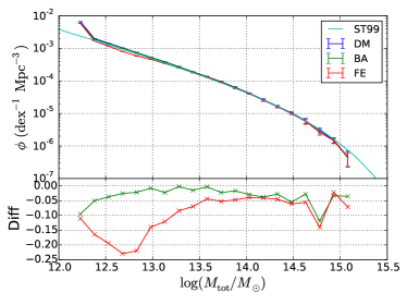
Figure 1.— Top panel: We plot the halo mass functions at $z=0$ measured from our set of simulations. The horizontal axis represents total mass of halos which include dark matter, gas and star particles. The blue, green and red line corresponds to simulation results averaged over 10 realizations of DM model, BA model and FE model, respectively. The error bars represent the standard deviation of the ten realizations for each model. The cyan line shows model prediction by Sheth & Tormen (1999). Bottom panel: The fractional difference of baryonic models from the fiducial model.

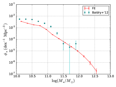
Figure 2.— Galaxy stellar mass functions at $z=0$. The cyan points show observational estimates from Baldry et al. (2012). The red line illustrates the result from FE simulation averaged over 10 realizations and the error bars represent the standard deviation.

In order to check basic statistics of our simulations, we measure halo mass function for each model and stellar mass function for FE model. We run a friends-of-friends (FoF) halo finder SubFind (Springel et al., 2001; Dolag et al., 2009) to identify halos in simulations. For our simulations with baryons, the procedure is different from that for CDM only simulation. First, using only dark matter particles, we find FoF groups which contain more than 31 particles. Next, we find gas particles for BA model and gas and star particles for FE model linked with a dark matter particle which belongs to a FoF group. Finally, we separate each FoF group into a central halo and substructures. In FE model, the stellar component of a halo is called ‘galaxy’ and ‘halo’ includes the baryonic components and dark matter. Figure 1 and 2 represent halo and stellar mass functions measured from simulations at $z=0$. We compare the simulation result with theoretical prediction of Sheth & Tormen (1999). Figure 1 clearly shows our simulation results are well described by the theoretical prediction over the typical cluster mass scale, while there are appreciable discrepancies between DM and FE simulations in the halo mass of less than $\sim 10^{13.5}M_{\odot}$. This is partly induced by SN explosions and/or stellar winds. Energy released by SN explosions or stellar winds expel gas particles from the halo but massive halos can retain the particles by the deep gravitational potential well. As a result, the mass function for our FE model is slightly smaller at small masses. We also compare the stellar mass functions of our simulation results and the observation of galaxy stellar mass function in Baldry et al. (2012). The stellar mass distribution in our FE model is in reasonable agreement with the observation at $z\sim 0$. Because we adopt a simpler model than the original implementation of Okamoto et al. (2014) that includes radiation pressure feedback, our FE run produces less small-mass galaxies. Also, our simulation results are inaccurate at stellar masses less than $\sim 10^{10}M_{\odot}$, because such small galaxies contain only a few star particles. These small discrepancies are, however, unimportant in the present paper because we draw our main conclusions through comparisons of multiple sets of simulations with and without baryonic components, rather than through comparisons of different feedback models.

3.2. Ray-tracing simulations

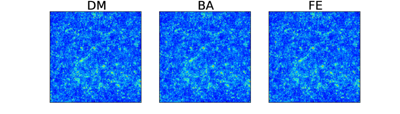
Figure 3.— We show sample convergence maps of DM, BA and FE simulations without noise and smoothing. Red or blue area corresponds to high or low convergence respectively. There are many red points, which are identified as peaks.

For ray-tracing simulations of gravitational lensing, we utilize multiple simulation boxes to generate light-cone outputs similarly to White & Hu (2000), Hamana & Mellier (2001), and Sato et al. (2009). Details of the configuration are found in the last reference.

We place the simulation outputs to fill the past light-cone of a hypothetical observer with an angular extent $5^{\circ}\times 5^{\circ}$, from $z=0$ to 1. The angular grid size of our maps is set to be $5^{\circ}/4096\sim 0.073$ arcmin. We randomly rotate and shift the simulation boxes in order to avoid the same structure appearing multiple times along a line-of-sight. In total, we generate 100 independent lensing maps for the source redshift of $z_{\rm source}=1$ . We show an example of convergence maps obtained from each baryonic model (DM, BA, and FE) in Figure 3. Note that each realization of three models use the same random seed when we generate initial conditions and multiple planes.

In order to make the mock lensing maps more realistic, we add random gaussian noises as shape noise to the simulated convergence data (e.g., Kratochvil et al. (2010) and Shirasaki et al. (2012)):

$$\langle\kappa_{\mathrm{noise}}(x_{1},x_{2})\kappa_{\mathrm{noise}}(x_{1}^{\prime},x_{2}^{\prime})\rangle=\frac{\sigma_{\gamma}^{2}}{n_{\mathrm{gal}}A_{\mathrm{pix}}}\delta_{x_{1},x_{1}^{\prime}}\delta_{x_{2},x_{2}^{\prime}},$$

where $\delta_{x,y}$ is the Kronecker delta symbol, $n_{\mathrm{gal}}$ is the number density of source galaxies, $\sigma_{\gamma}$ is the rms of shape noise and $A_{\mathrm{pix}}$ is the solid angle of a pixel. In the following, we adopt $\sigma_{\gamma}=0.4,n_{\mathrm{gal}}=30\ \mathrm{arcmin}^{-2}$. These values are expected to be typical for HSC survey.

As described in Section 2.1.2 and 2.1.3, smoothing is required to measure non-local statistics of convergence from noisy WL data. For a given smoothing scale $\theta_{G}$, the rms of the shape noise after gaussian smoothing is given by van Waerbeke (2000)

$$\sigma_{\mathrm{noise}}=0.0291\left(\frac{\sigma_{\gamma}}{0.4}\right)\left(\frac{\theta_{G}}{1\,{\rm arcmin}}\right)^{-1}\left(\frac{n_{\mathrm{gal}}}{30\,{\rm arcmin}^{-2}}\right)^{-1/2}.$$

(25)

4. ANALYSIS

We quantify the effects of the baryonic processes on weak lensing analyses in terms of errors and bias in cosmological parameter estimation. We consider primarily a lensing survey with a sky coverage of 1400 deg², i.e., the ongoing wide-field survey by Subaru Hyper Suprime-Cam (HSC). In the following, we describe in detail the calculation of the ensemble averages of three statistics and the covariance matrix in order to derive statistical implications and to estimate cosmological parameters $\bm{p}=(\Omega_{\textrm{m}},w,10^{9}A_{s})$.

4.1. Theoretical model and covariance of lensing statistics

Table 2The configuration of bins for each observable

Observable	Range	No. of bins
PS	$100\leq\ell\leq 2000$	10
MP	$1.0\leq\mathcal{K}_{\mathrm{peak}}/\sigma_{\mathrm{noise}}\leq 3.0$	10
HP	$3.0\leq\mathcal{K}_{\mathrm{peak}}/\sigma_{\mathrm{noise}}\leq 5.0$	10
MFs	$-3.0\leq(\nu-\langle\mathcal{K}\rangle)/\sigma_{0}\leq 3.0$	10 for each

First, we calculate the theoretical template and covariance of the WL statistics using our ray-tracing simulations. The configuration of bins are given in Table 2. The model template and covariance are based on our DM models. Later, we examine the baryonic effects on WL cosmological analysis by comparison with DM model and two baryonic models.

We represent the data vector as $N_{i}$ and denote the dimension of the data vector as $n$. Note that $n$ can be larger than ten, when multiple observables are combined. We derive theoretical prediction of lensing statistics by averaging over $R=100$ realizations:

$$\langle N_{i}(\bm{p})\rangle\simeq\bar{N_{i}}(\bm{p})\equiv\frac{1}{R}\sum_{r=1}^{R}N_{i}(r,\bm{p}).$$ (26)

In order to consider the cosmological parameter dependence on $N_{i}$, we employ linear interpolation based on DM models with seven different cosmologies. Thus, we obtain the theoretical model of $N_{i}$ for a given cosmological model as follows:

$$\bar{N_{i}}(\bm{p})=\bar{N_{i}}(\bm{p}^{0})+\sum_{\alpha}\frac{\bar{N_{i}}(\bm{p}^{\alpha+}_{\alpha})-\bar{N_{i}}(\bm{p}^{\alpha-}_{\alpha})}{p^{\alpha+}_{\alpha}-p^{\alpha-}_{\alpha}}(p_{\alpha}-p^{0}_{\alpha}),$$

where $\alpha$ runs 1 to 3 and the superscript 0 means fiducial value $\bm{p}^{0}=(0.279,-1.0,2.41)$. $\bm{p}^{\alpha\pm}$ represents a vector with one parameter with a higher or lower value; for example $\bm{p}^{1+}=(0.302,-1.0,2.41)$ (the other parameter values are given in Table.1).

The covariance matrix of the data vector $N_{i}$ on 25 deg² maps is estimated as

$$C_{ij}(\bm{p})=\frac{1}{R-1}\sum_{r=1}^{R}[N_{i}(r,\bm{p})-\bar{N_{i}}(\bm{p})][N_{j}(r,\bm{p})-\bar{N_{j}}(\bm{p})].$$

(28)

We ignore the cosmological dependence of $C(\bm{p})$ (see, e.g., Eifler et al., 2009) and hence evaluate the covariance matrix by using the fiducial model, i.e. $C(\bm{p}^{0})$. For the fiducial HSC survey, we simply scale the covariance matrix by survey area, by multiplying the covariance matrix $C_{ij}(\bm{p}^{0})$ in Eq. (28) by a factor of $25/1400$. When calculating the inverse covariance, we include a debiasing correction, the so-called Anderson-Hartlap factor $\alpha=(R-n-2)/(R-1)$ (Hartlap et al., 2007), where $R$ is the number of realizations and $n$ is the dimension of the data vector.

4.2. Fisher analysis

Fisher analysis gives a simple forecast for statistical confidence level of three cosmological parameters ($\Omega_{\mathrm{m}},w,10^{9}A_{s}$) with WL statistics. The Fisher matrix is given by

$$F_{ij}=\frac{1}{2}\mathrm{Tr}[A_{i}A_{j}+C^{-1}M_{ij}],$$ (29)

where $A_{i}=C^{-1}\partial C/\partial p_{i}$, $M_{ij}=2(\partial\bm{N}/\partial p_{i})(\partial\bm{N}/\partial p_{j})^{T}$. The first term vanishes when the cosmological dependence is weak (Eifler et al., 2009). To compute the second term, the first derivative is evaluated by the first order finite difference, which is given by

$$\frac{\partial\bm{N}}{\partial p_{i}}\simeq\frac{\bm{\bar{N}}(\bm{p}^{i+}_{i})-\bm{\bar{N}}(\bm{p}^{i-}_{i})}{p^{i+}_{i}-p^{i-}_{i}}.$$ (30)

Then, the marginalized error over the other two parameters is given by

$$\sigma_{i}=\sqrt{(F^{-1})_{ii}}.$$ (31)

4.3. Mock lensing surveys

In order to make a realistic forecast in upcoming HSC survey, we employ the bootstrap method as in Yang et al. (2013). Since our suite of WL maps consist of one hundred 25 deg² maps, we randomly choose $1400/25=56$ realizations from one hundred 25 deg² WL maps. Repeating this procedure one thousand times, we can get one thousand ‘mock’ HSC WL maps. The resulting maps are based on the fiducial cosmological model but we also have the same set from simulations with the different baryonic effects. Lensing statistics of interest (i.e. PS, peak counts and MFs) in HSC surveys are evaluated by averaging each statistics on a 25 deg² map over 56 realizations.

We then utilize the HSC observables derived in this way to investigate the impact of baryonic effects on parameter estimation. We perform $\chi^{2}$ minimization to $N_{i,{\rm HSC}}$ as follows:

$$\chi^{2}(r,\bm{p},m)=\sum_{i,j}\varDelta N_{i}(C^{-1})_{ij}\varDelta N_{j},$$ (32)

where $\varDelta N_{i}\equiv N_{i,{\rm HSC}}^{m}(r)-\bar{N}_{i}(\bm{p})$, $r$ is the index of realizations and $1\leq r\leq 1000$, $\bar{N}_{i}$ represents the theoretical model of $N_{i}$ for our dark matter only (DM) model, and $m$ represents the difference of model of baryonic physics, i.e., BA and FE. Suppose we calculate the $i$-th data $N_{i,{\rm HSC}}$ from a dark matter only convergence map ($m=\mathrm{DM}$), we should then find the resulting best-fit points distribute around the fiducial point $\bm{p}^{0}=(0.279,-1.0,2.41)$. However, when one considers the case of $m=\mathrm{BA\ or\ FE}$, the center of the distribution of best-fit values could be biased in parameter space of $\bm{p}$ if baryonic effects induce discrepancies between $N_{i,{\rm HSC}}$ and $\bar{N}_{i}(\bm{p}^{0})$. That means $\chi^{2}$ values calculated from Eq. (32) do not follow $\chi^{2}$ distribution for baryonic models because the ensemble mean and the covariance matrix are computed from the fiducial model, not baryonic models.

There is another way to estimate the bias of parameter estimation. The parameter biases of the BA and FE models from fiducial parameters can be computed in the following manner (see, e.g., Huterer et al., 2006):

$$\delta p_{\alpha}=\sum_{\beta}F^{-1}_{\alpha\beta}\sum_{i,j}[\bar{N}_{i}^{m}-\bar{N}_{i}(\bm{p}^{0})](C^{-1})_{ij}\frac{\partial N_{j}}{\partial p_{\beta}},$$ (33)

where $F$ is the fisher matrix given by Eq. (29) and $\bar{N}_{i}^{m}$ represents the average of $N_{i}$ over 100 convergence maps for $m=\mathrm{BA\ and\ FE}$.

In the following, we quantify the baryonic effects on parameter estimation with WL surveys by considering the distribution of $\chi^{2}$ in Eq. (32) and $\delta p_{\alpha}$ in Eq. (33) for our BA and FE models. We then compare the bias of parameter estimations with the marginalized error given in Eq. (31).

5. RESULTS

5.1. Baryonic effect on convergence statistics

We summarize the main results of the baryonic effects on WL statistics in Figure 4, 5 and 6.

Figure 4 show PS from our maps, where DM, BA and FE models are indicated by blue, green and red lines respectively. We also show the theoretical prediction by the cyan line which is calculated by Eq. (9) with the modeling of matter power spectrum, essentially an modified HaloFit, of Takahashi et al. (2012) We plot the shot noise contribution in the bottom panel as the dashed magenta line. The error bars represent the standard deviations over one hundred maps. The top and bottom panel represents to results from the maps with and without noises, respectively. The lower portion in each panel shows the fractional differences of BA and FE models with respect to the DM model.

Power spectrum

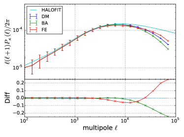
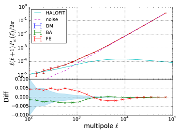
Figure 4.— We plot the convergence power spectrum from one hundred convergence maps. The top and bottom panel show the result without and with noise and smoothing. The solid cyan line shows the model prediction using HaloFit of Takahashi et al. (2012). The measured powers from simulations are slightly smaller than the result of HaloFit due to finite box effect. The dashed magenta line in the noisy case shows the power spectrum of the noise. In the lower portion of each panel, we plot the fractional differences from the fiducial model and the blue filled region corresponds to the expected statistical error of DM model when one measures the power spectrum from one hundred 1400 deg² maps. Note that this region does not correspond to the error bar, i.e. the standard deviation, shown in the upper panel that is measured from our sample of 25 deg² maps. And in the top panel, this expected error of power spectrum from noise free maps is so small that it does not appear clearly.

Compared with DM model, gas pressure suppresses small-scale ($\ell>10000$) structures in BA model. On the other hand, in FE model feedback processes are efficient at the scales of $2000<\ell<10000$ but cooling processes enhance the convergence power at the smaller scale $\ell>20000$. These features by cooling and feedback processes are consistently found by Semboloni et al. (2011); Mohammed et al. (2014). However, the strength of the baryonic enhancement and suppression is different, because of the details of baryonic physics implementations and also partially because of the difference of cosmological parameters.

Peak count

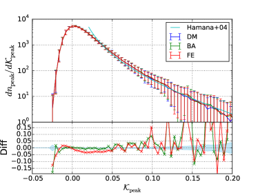
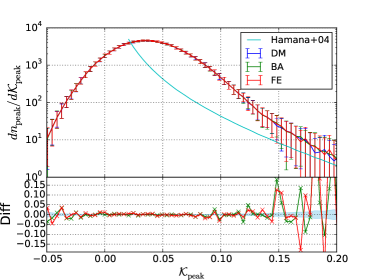
Figure 5.— The number of peaks per unit square degree. The top and bottom panel shows the result without and with noise. The solid cyan line shows the model prediction of peaks by Hamana et al. (2004), which assumes that the halo mass function is described by Sheth & Tormen (1999) and the density profile of halos follow Navarro-Frenk-White profile (Navarro et al., 1996, 1997a). The lower portion in each panel shows the fractional difference from the fiducial model. The blue filled region represents expected Poisson error of DM model from one hundred 1400 deg² maps.

Figure 5 shows the peak counts measured from the simulated convergence maps for the three models. We use the same combination of line colors as in Figure  4. The error bars represent standard deviations from one hundred maps. The lower portion in each panel shows the fractional difference of BA and FE models with respect to DM model, and the shaded region indicates the Poisson error of the fiducial model, i.e. the square root of the number of peaks within a bin, In this figure, we employ 5 bins per unit S/N ratio $\nu/\sigma_{\mathrm{noise}}$, the peak height of convergence $\nu$ divided by $\sigma_{\mathrm{noise}}$. For the analytical prediction, we adopt the model of Hamana et al. (2004) with Sheth-Tormen (Sheth & Tormen, 1999) mass function and Navarro-Frenk-White dark matter density profile (Navarro et al., 1996, 1997a). We assume the relation between the halo mass and concentration parameter as in (Hamana et al., 2012),

$$c(M,z)=7.26\left(\frac{M}{10^{12}M_{\odot}/h}\right)^{-0.086}(1+z)^{-0.71},$$ (34)

In Figure 5, medium peaks (MPs) correspond to the peaks with $0.03\lower 2.15277pt\hbox{$\;\buildrel<\over{\sim}\;$}\mathcal{K}_{\rm peak}\lower 2.15277pt\hbox{$\;\buildrel<\over{\sim}\;$}0.09$, while high peaks (HPs) are those with $0.09\lower 2.15277pt\hbox{$\;\buildrel<\over{\sim}\;$}\mathcal{K}_{\rm peak}\lower 2.15277pt\hbox{$\;\buildrel<\over{\sim}\;$}0.15$. HPs are typically associated with massive halos with the mass of $\sim 10^{14}M_{\odot}$. The number of HPs is less affected by baryonic effects because the baryonic processes do not cause very strong effect to change the number of such massive halos, as seen in Figure 1. MPs often originate from multiple halos with masses of $10^{12}-10^{13}M_{\odot}$ aligned in the line of sight direction. Baryonic physics, such as SN and AGN feedback, reduce the masses of these halos (see Section 2.1.2). Hence the baryonic effects would decrease the number of MPs, but the difference is largely made unimportant in the noisy convergence maps because MPs are affected significantly by shape noise (Yang et al., 2011).

Minkowski Functionals

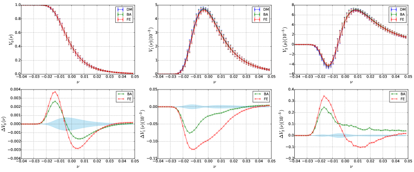
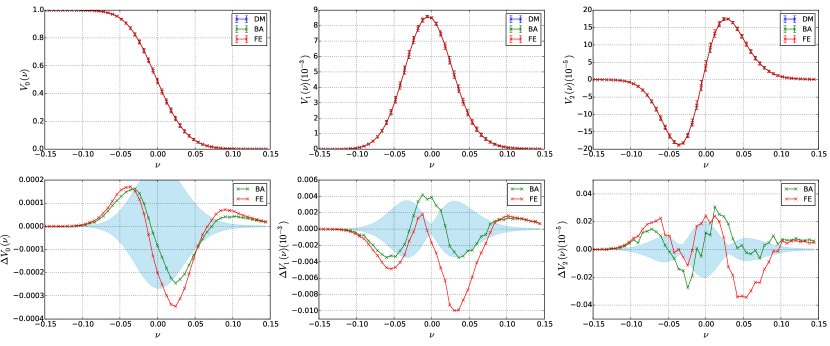
Figure 6.— The three MFs averaged over one hundred convergence maps. Panels in the first and the second rows show the results without noise whereas the third and the fourth rows are for those with noise. The error bars show the standard deviation of one hundred maps. Note that the range of threshold $\nu$ is different between the noise-free and noisy cases. The blue filled region corresponds to the expected statistical error of DM model from one hundred 1400 deg² maps.

Figure 6 show the MFs computed from our maps of DM, BA and FE models. Again we use the same color for each model as in the previous figures. The MFs $V_{0}$, $V_{1}$ and $V_{2}$ are plotted from left to right. The upper (lower) two rows represent results from noise-free (noisy) maps. Panels in the second and fourth row show the difference of BA and FE models from the DM model. The error bars represent standard deviations from one hundred maps. We employ 5 bins per unit $\nu^{\prime}=(\nu-\langle\mathcal{K}\rangle)/\sigma_{0}$. It is useful to calculate the expectation values for a Gaussian random field (Eqs. (18)-(20)) in order to understand the overall feature of MFs. In Eqs. (18)-(20), the spectral moments $\sigma_{0}$ and $\sigma_{1}$ can be calculated from the convergence power spectrum as

$$\sigma_{p}^{2}=\int\frac{{\rm d}^{2}\ell}{(2\pi)^{2}}\ell^{2p}P_{\kappa}(\ell)|\tilde{W}_{G}(\ell;\theta_{G})|^{2},$$ (35)

where $\tilde{W}_{G}$ represents the Fourier transform of Eq. (12), which is given by $\exp\left(-\ell^{2}\theta_{G}^{2}/4\right)$. Note that $\tilde{W}_{G}$ decreases exponentially at $\ell\lower 2.15277pt\hbox{$\;\buildrel>\over{\sim}\;$}20000\times(1\,{\rm arcmin}/\theta_{G})$. ¿From the result shown in Figure 4, we expect that $\sigma_{0}$ of BA and FE models is smaller than that of DM model but $\sigma_{1}$ would be nearly the same. We confirm this notion by direct measurement of $\sigma_{0}$ and $\sigma_{1}$ from our 100 maps. It is important to test whether the differences between the models are attributed to $\sigma_{0}$. In the above analysis, we measured MFs in terms of normalized threshold $\nu^{\prime}$ because, if the difference is largely owing to variation of $\sigma_{0}$, the normalization would absorb all or most of the differences. The difference in the MFs becomes indeed slightly smaller with the normalization, but does not vanish completely. Therefore, the baryonic processes apparently affect the MFs. It is necessary to develop further analysis beyond Gaussian description to explain the difference of MFs between baryonic and fiducial models.

5.2. Fisher forecast and bias of cosmological parameters

Table 3The marginalized errors and biases

Data statistics	$\delta\Omega_{\textrm{m}}$	$\delta w$	$\delta 10^{9}A_{s}$
Fisher forecast marginalized $1\sigma$ error
PS	$0.0275$	$0.276$	$1.01$
MP	$0.00853$	$0.110$	$0.0557$
HP	$0.0129$	$0.118$	$0.0971$
$V_{0}$	$0.00678$	$0.0711$	$0.0831$
$V_{1}$	$0.00767$	$0.0911$	$0.0931$
$V_{2}$	$0.00912$	$0.115$	$0.0718$
$V_{0}+V_{1}+V_{2}$	$0.00439$	$0.0513$	$0.0521$
PS+MP+HP	$0.00478$	$0.0520$	$0.0371$
PS+MP+$V_{0}$	$0.00372$	$0.0391$	$0.0412$
PS+HP+$V_{0}$	$0.00547$	$0.0456$	$0.0662$
Parameter bias of BA
PS	$0.00104$	$0.000285$	$-0.0342$
MP	$-0.00280$	$-0.0394$	$-0.0187$
HP	$-0.00745$	$-0.0648$	$0.0278$
$V_{0}$	$-0.00385$	$-0.0471$	$0.0435$
$V_{1}$	$-0.00349$	$0.0147$	$0.101$
$V_{2}$	$-0.00518$	$-0.0479$	$0.0169$
$V_{0}+V_{1}+V_{2}$	$-0.00271$	$0.00352$	$0.0477$
PS+MP+HP	$-0.00115$	$-0.0145$	$-0.0134$
PS+MP+$V_{0}$	$0.000493$	$0.00803$	$0.00428$
PS+HP+$V_{0}$	$0.00148$	$0.0261$	$0.00488$
Parameter bias of FE
PS	$-0.00171$	$-0.0172$	$0.0139$
MP	$-0.00591$	$-0.0616$	$0.00536$
HP	$-0.00668$	$-0.0610$	$0.0347$
$V_{0}$	$-0.000951$	$-0.00112$	$0.0543$
$V_{1}$	$-0.00559$	$0.00157$	$0.120$
$V_{2}$	$-0.00182$	$0.0135$	$0.0342$
$V_{0}+V_{1}+V_{2}$	$-0.000412$	$0.0347$	$0.0481$
PS+MP+HP	$-0.00594$	$-0.0587$	$0.0156$
PS+MP+$V_{0}$	$-0.00288$	$-0.00899$	$0.0544$
PS+HP+$V_{0}$	$0.000589$	$0.0136$	$0.0241$

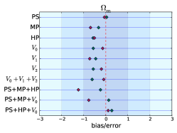
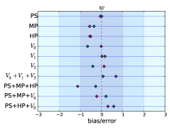
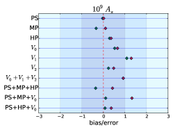
Figure 7.— The parameter biases divided by marginalized errors. Green and red points correspond to BA and FE models respectively. The biases caused when using only one observable are mostly within $1\sigma$. However, in combined analyses, e.g. PS+MP+HP, the resulting bias can exceed the marginalized $1\sigma$ error.

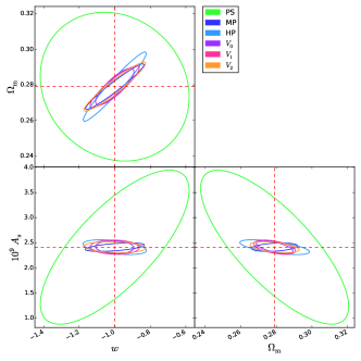
Figure 8.— We compare the 1$\sigma$ confidence regions calculated from Fisher forecast using six observables separately. The confidence region from PS (green line) is clearly the largest. The other non-local statistics yield substantially smaller confidence regions.

We show the results of our parameter estimation in Figures  9 to 11. In each figure, we show two-dimensional error contours marginalized over the other parameter. The blue, green and red dots indicate the best-fit values for DM, BA and FE models, respectively. Red dashed lines represent the fiducial values. Note that in these three figures, the plotted parameter range is adjusted according to the size of the forecast circle for the observable. In order to make comparison between the figures easy, we show the $1\sigma$ confidence regions of six observables in the same scale in Figure 8. The biases and marginalized errors of parameters are summarized in Table 3 and Figure 7. In Figure 7, green and red points show the biases divided by the marginalized errors for BA and FE models. To check the accuracy of our code, we also present results from the fiducial simulation. We plot results obtained from $\cal{K}$ maps with shape noise.

In the following, we summarize the baryonic effects on parameter estimation with different convergence statistics.

Power spectrum

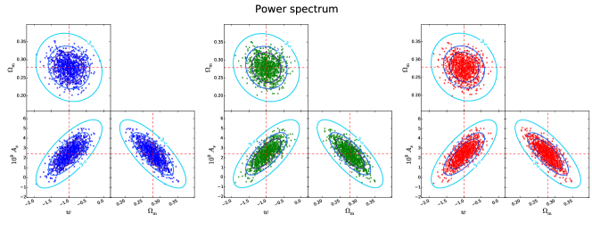
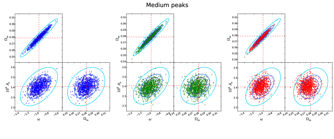
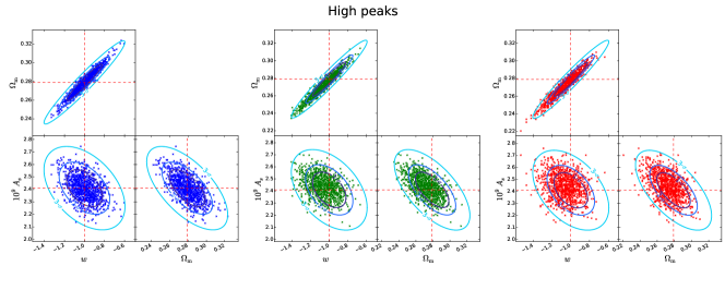
Figure 9.— Error contours and best-fit points using PS and peak counts. Blue, green and red dots indicate the best fit values for each realization of our DM, BA and FE model suites. Light blue, blue and deep blue contour show $1\sigma$, $2\sigma$ and $3\sigma$ confidence boundary obtained in the Fisher analysis of DM model (described in Sec. 4.2), respectively. The discrepancy between the distribution of green or red points and the blue confidence regions is attributed to “baryonic effects”. Red dashed lines represent fiducial parameter values.

The top three panels in Figure 9 show the results of parameter estimation for three (DM, BA, FE) models using only PS. We find only small bias caused by the baryonic physics. That is because, with realistic ground-based surveys PS can be measured accurately at low $\ell$ about $2000$ at most, which is the maximum multipole used in our estimation. The difference between the fiducial and baryonic models appears at the small scale. The PS amplitude and the shape at $\ell\lower 2.15277pt\hbox{$\;\buildrel<\over{\sim}\;$}2000$ are not significantly affected by the baryonic physics. Previous studies (Yang et al., 2013; Mohammed et al., 2014) also examined differences due to the choice of the maximum multipole. In our result, the difference at large scale is quite small whereas noise dominates at smaller angular scales, where PS can not be measured accurately. For this reason, we fix the maximum multipole at $\ell=2000$. Then the baryon effects on PS is negligible in cosmological parameter estimation using PS.

Peak count

The medium (bottom) three panels in Figure 9 show the results using only MPs (HPs). As we have discussed above, medium height peaks are also dominated by intrinsic shape noise but still have cosmological information. High peaks have nearly one-to-one relation with massive halos, whose masses are less affected by the baryonic processes. Interestingly, we find that both MPs and HPs induce biased parameter estimation of $w$ with a level of $\sim 0.56\sigma$ and $0.52\sigma$, respectively, for FE model. The bias may be partly originated from the baryonic effect on the shape of massive halos. Massive halos tend be rounder when baryonic processes are included (e.g., Kazantzidis et al., 2004). Then the height of a peak associated with a single halo is reduced, and so may be the peak counts at $\cal{K}\sim$ $0.0-0.05$.

Minkowski Functionals

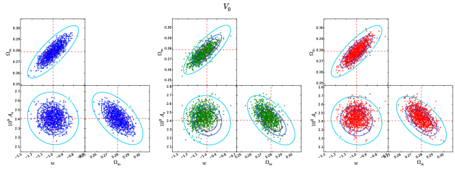
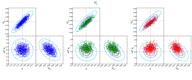
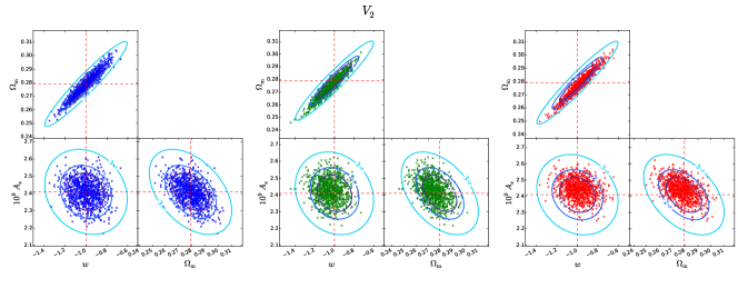
Figure 10.— Error contours and best-fit points using MFs.

Figure 10 shows the results using each of the three MFs, $V_{0},V_{1},V_{2}$. The center of the dots is shifted in the respective parameter space; significant parameter bias can be caused by the baryonic effects. Note that the absolute shift itself is not very large, but that the bias with respect to the error circle is appreciable (see Fig. 8 for the relative size of the error circles). When one constructs the theoretical template of MFs without the modeling of baryonic physics, analyses using $V_{0}$, $V_{1}$ and $V_{2}$ cause the biased estimation of $w$ with a level of $\sim 0.016\sigma$, $0.017\sigma$, and $0.12\sigma$, respectively, for FE model. Although it is difficult to explain the origin of this bias completely, we expect the following two effects can be responsible for the biased parameter estimation: (i) the change of variance of $\cal{K}$ (i.e. $\sigma_{0}$) and (ii) the change in halo shape. More detailed modeling with an analytic halo approach would be useful to investigate the relation between the property of dark matter halos and lensing MFs. This is along the line of our ongoing study using a large set of cosmological simulations.

Combined analysis

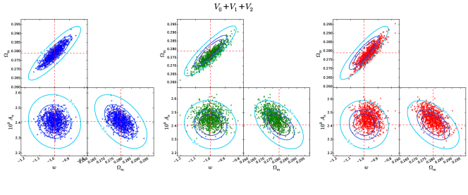
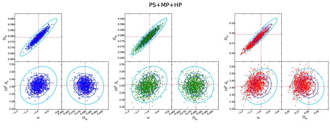
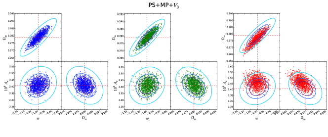
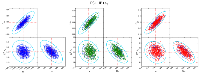
Figure 11.— Error contours and best-fit points for combined analysis

Let us consider a combined analysis with multiple observables in order to tighten the error and possibly mitigate the bias due to baryonic effects.

Our combination of the observables are of the following four types: (i) all the MFs, (ii) PS and peak counts, (iii) PS, MPs and $V_{0}$, and (iv) PS, HPs and $V_{0}$. The last two are examples of less biased combinations of the statistics. We propose the two combinations that are expected to cause small net bias of parameters on the basis of the result of Eq. (33). The basic idea is to find a combination of observables with biases in the opposite directions in parameter space.

Figure 11 shows the results of the above combined analysis. All of combined analysis presented here can tighten forecast errors, i.e. they can effectively extract more cosmological information. Some combinations, e.g. PS and peak counts, is largely affected by biases by baryonic effects. This degrades parameter constraints of combined analysis. However, if we adopt, e.g. PS+HPs+$V_{0}$, such combination can mitigate the bias by baryonic effects. When all the statistics cause biases with the same sign (e.g., for $10^{9}A_{s}$), it is safe to combine those with small biases. On the other hand, there is still a possibility of causing large biases by combined analysis, if one include statistic(s) whose bias is very large. In general, cosmological parameters are degenerated with each other and thus it is not trivial to determine the best combination for multiple parameters. The above case focusing on a single may serve as a useful guide for combined analysis when parameter degeneracy is not strong. We further discuss with a simple example with details in multi-dimensional parameter space of the formalism in Appendix.

6. CONCLUSION AND DISCUSSION

We have studied baryonic effects on WL statistics using a suite of cosmological simulations that incorporate galaxy formation processes. Various baryonic processes are implemented in our code, such as gas cooling, star formation, and stellar feedback. These processes themselves are important subjects of research and the model uncertainties with free parameters are still controversial, but such simulations can be used to quantify the baryonic effect, or at least to compare the WL statistics with those calculated from dark matter only simulations. We focus on cosmological parameter estimation using WL statistics. To this end, we made realistic mock observations by performing ray-tracing simulations through the non-linear density fields with the size of survey region over 1000 square degrees.

We have studied three statistics, PS, peak counts and MFs, calculated directly from mock lensing maps with baryons and compare them with the results from our ‘fiducial’ dark matter only simulations. The PS deviate appreciably at $\ell\lower 2.15277pt\hbox{$\;\buildrel>\over{\sim}\;$}7000$ from the fiducial model due to the baryonic processes. This feature is also seen in previous studies, e.g., Semboloni et al. (2011). The shape noise dominates, however, over the baryonic effects at the small angular scales and thus the baryonic effects are not critical in practice in the analysis using PS. Peak counts in convergence maps are also affected because the height of a peak is sensitive to the mass and the density profile of the corresponding halo. Stellar feedback can effectively reduce the mass of small galaxy halos, which results in decrease of the number of medium height peaks. High peaks are less affected by the stellar feedback effects because the mass distribution in massive, cluster-size halos are not significantly changed by the stellar feedback. Yang et al. (2013) examine the influence on peak counts of the enhancement of halo concentration parameter, motivated by radiative cooling. They show that the number of HPs is increased accordingly, while the number of MPs is mostly unaffected. We do not see the feature in our high peak-counts, probably because our simulations include not only radiative cooling but also supernova and stellar feedback that can compensate, at least partially, the condensation of baryons. Finally, MFs are morphological statistics and thus are promising as a probe of the baryonic effects that change the internal matter distribution of halos. The shape noise again substantially affects MFs owing to the effectively increased $\kappa$-variance. Also, the smoother distribution of the gaseous components causes the overall feature of the MF smoother, especially in our BA model (see Fig. 6).

We have considered three kinds of statistics as probes of cosmological parameters. When we use only one of them, the parameter bias due to the baryonic effects is not significant. Most of the biases are found to be within 1$\sigma$ error for the fiducial 1400 square degree survey. It is expected that, with the upcoming Subaru HSC survey, cosmological parameters can be determined without being significantly compromised by baryonic processes as long as a single statistic is used. However, because the statistical error itself becomes small, roughly in proportion to the increase of square root of the survey area, even a very small bias would become critical for future surveys with a half or an all sky coverage. The overall bias can appear relatively amplified when a combination of a few or more statistics are used because the expected error of the parameters becomes small and the bias remains the same. For example, when using both PS and peak counts, the parameter bias for $w$ is over $1\sigma$. Clearly, such bias needs to be well understood before analyzing real observational data. It is also desirable to find a combination of statistics that yields both high precision and small bias. If we consider only one parameter, a best way would be to combine statistics such that their respective biases can cancel each other (see Figure 7). Unfortunately, it is generally non-trivial to estimate parameter bias in a multi-dimensional space because the degeneracy between multiple parameters leads to complicated dependence on parameters. We suggest to try all possible combinations and study in detail, as has been done in the present paper in the case with only a few statistical measures. Among the combinations we have tested, we find the combination of PS, one of peak counts and $V_{0}$ gives high precision and yet robust results against the baryonic effects. Furthermore, all of the quantities can be predicted accurately by analytic models. Takahashi et al. (2012) studied non-linear PS using HaloFits approach. Hamana et al. (2004) employs one-to-one relation that NFW-halo corresponds to a peak but this approach is only valid at high S/N ratio ($\lower 2.15277pt\hbox{$\;\buildrel>\over{\sim}\;$}4$) peaks. For low S/N ratio peaks, this relation breaks down. Das & Ostriker (2006) studied the probability distribution function of convergence using fitting formula motivated by the log-normal distribution. This probability distribution function is directly related with $V_{0}$. In recent studies, Fedeli (2014); Fedeli et al. (2014); Mohammed et al. (2014) study baryonic effects on PS using a halo model. It would be interesting to study the link between other two statistics and properties of halos by extending the halo model approach. We leave it as a future work. The connection between halo properties and WL statistics is also interesting in that we can possibly observe halo properties through WL statistics.

Our results suggest that the non-local statistics have a stronger parameter constraining power than PS, even when baryonic effects are taken into account. However, one needs to be careful in using the non-local statistics. Theoretical frameworks to predict PS have been well developed through both numerical and analytic approach. In realistic observations, the shear measurement itself is clean and local, especially when compared with the other non-local statistics. Overall, PS is the most studied statistic and it is intuitively easy to understand based on physics; $P_{\kappa}(\ell)$ is a direct measure of the fluctuations at a given scale $\ell$. Although some numerical studies (Kratochvil et al., 2012; Shirasaki & Yoshida, 2014) suggest that non-local statistics would be useful to make tight cosmological constraints, there are intrinsic difficulties to derive analytical models for MFs and peak counts. Hence it is not straightforward to interpret the non-local statistics and their dependence on cosmological parameters. In order to rely on the non-local statistics with real data, full comprehension of systematic uncertainties induced by observational effects is necessary. Clearly, these issues are worth studying further in order to explore fully the applicability of the non-local statistics. In this paper, we have clarified the theoretical uncertainty of non-local statistics due to baryonic processes. Our result is a key to the precise application of non-local statistics of cosmic shear for cosmological analyses with the unprecedented large surveys.

Appendix A Combined analysis in one-dimensional parameter space

We present the criterion for the choice of observables for a combined analysis in a simplified case. The parameter bias of a combined analysis is given by

$$\delta\hat{p}_{\alpha}=(\hat{F})^{-1}_{\alpha\beta}\sum_{i,j}(N_{i}-\bar{N}_{i})(\hat{C})^{-1}_{ij}\frac{\partial N_{j}}{\partial p_{\beta}},$$ (A1)

where $\hat{F}$ and $\hat{C}$ is the Fisher matrix and the covariance matrix in the case of combined analysis with several observables. Assuming that each observable is independent, one can write $\hat{p}_{\alpha}$ as

$$\delta\hat{p}_{\alpha} = (\hat{F})^{-1}_{\alpha\beta}\sum_{i,j,s}(N^{s}_{i}-\bar{N}^{s}_{i})(C^{s})^{-1}_{ij}\frac{\partial N^{s}_{j}}{\partial p_{\beta}}$$ (A2)

$$= (\hat{F})^{-1}_{\alpha\beta}\sum_{s}(F^{s})_{\gamma\beta}\delta p_{\gamma}^{s},$$ (A3)

where $F^{s}$ and $C^{s}$ is the Fisher matrix and the covariance matrix for each observable $s$, e.g. $s=$PS.

For one-dimensional parameter space, we can simplify Fisher matrices,

$$F^{s}\to\sigma_{s}^{-2},\ \hat{F}^{s}\to\sum_{s}\sigma_{s}^{-2},$$ (A4)

where $\sigma_{s}$ is the forecast error with the observable $s$. Hence, the expected bias with a combined analysis is given by

$$\delta\hat{p}=\left(\sum_{s^{\prime}}\sigma_{s^{\prime}}^{-2}\right)^{-1}\sum_{s}\frac{\delta p^{s}}{\sigma_{s}^{2}}.$$ (A5)

When the sum of $\delta p^{s}/\sigma_{s}^{2}$ vanishes, the net bias $\delta\hat{p}$ also vanishes. Therefore, a combination that makes the sum small is a good probe with less bias. We show the bias divided by the square of the error for each observable in Figure 12. For multi-dimensional parameter space, this procedure is not generally applicable because the degeneracy between different parameters gives additional terms to Eq. (A5). But when the degeneracy is not strong and the bias is not large, this condition gives the effective criterion for a less biased combination of observables in terms of cosmological parameters.

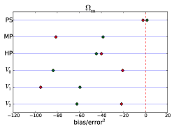
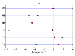
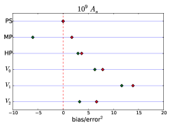
Figure 12.— The parameter biases divided by the square of marginalized errors. Green and red points correspond to BA and FE models respectively.

References

- Baldry et al. (2012) Baldry, I. K., Driver, S. P., Loveday, J., et al. 2012, Monthly Notices of the Royal Astronomical Society, 421, 621
- Bartelmann & Schneider (2001) Bartelmann, M., & Schneider, P. 2001, Physics Reports, 340, 291
- Beutler et al. (2014) Beutler, F., Saito, S., Seo, H.-J., et al. 2014, Monthly Notices of the Royal Astronomical Society, 443, 1065
- Crocce et al. (2006) Crocce, M., Pueblas, S., & Scoccimarro, R. 2006, Monthly Notices of the Royal Astronomical Society, 373, 369
- Das & Ostriker (2006) Das, S., & Ostriker, J. P. 2006, The Astrophysical Journal, 645, 1
- Dolag et al. (2009) Dolag, K., Borgani, S., Murante, G., & Springel, V. 2009, Monthly Notices of the Royal Astronomical Society, 399, 497
- Duffy et al. (2010) Duffy, A. R., Schaye, J., Kay, S. T., et al. 2010, Monthly Notices of the Royal Astronomical Society, 405, 2161
- Eifler et al. (2009) Eifler, T., Schneider, P., & Hartlap, J. 2009, Astronomy and Astrophysics, 502, 721
- Fan et al. (2010) Fan, Z., Shan, H., & Liu, J. 2010, The Astrophysical Journal, 719, 1408
- Fedeli (2014) Fedeli, C. 2014, Journal of Cosmology and Astroparticle Physics, 2014, 028
- Fedeli et al. (2014) Fedeli, C., Semboloni, E., Velliscig, M., et al. 2014, Journal of Cosmology and Astroparticle Physics, 2014, 028
- Hahn & Abel (2011) Hahn, O., & Abel, T. 2011, Monthly Notices of the Royal Astronomical Society, 415, 2101
- Hamana & Mellier (2001) Hamana, T., & Mellier, Y. 2001, Monthly Notices of the Royal Astronomical Society, 176, 169
- Hamana et al. (2012) Hamana, T., Oguri, M., Shirasaki, M., & Sato, M. 2012, Monthly Notices of the Royal Astronomical Society, 425, 2287
- Hamana et al. (2004) Hamana, T., Takada, M., & Yoshida, N. 2004, Monthly Notices of the Royal Astronomical Society, 350, 893
- Hartlap et al. (2007) Hartlap, J., Simon, P., & Schneider, P. 2007, Astronomy and Astrophysics, 464, 399
- Hilbert et al. (2009) Hilbert, S., Hartlap, J., White, S. D. M., & Schneider, P. 2009, Astronomy and Astrophysics, 499, 31
- Hinshaw et al. (2013) Hinshaw, G., Larson, D., Komatsu, E., et al. 2013, The Astrophysical Journal Supplement Series, 208, 19
- Huterer et al. (2006) Huterer, D., Takada, M., Bernstein, G., & Jain, B. 2006, Monthly Notices of the Royal Astronomical Society, 366, 101
- Jing et al. (2006) Jing, Y. P., Zhang, P., Lin, W. P., Gao, L., & Springel, V. 2006, The Astrophysical Journal, 640, L119
- Kaiser (1992) Kaiser, N. 1992, The Astrophysical Journal, 388, 272
- Kazantzidis et al. (2004) Kazantzidis, S., Kravtsov, A. V., Zentner, A. R., et al. 2004, The Astrophysical Journal, 611, L73
- Kilbinger (2014) Kilbinger, M. 2014, eprint arXiv:1411.0115
- Kilbinger et al. (2013) Kilbinger, M., Fu, L., Heymans, C., et al. 2013, Monthly Notices of the Royal Astronomical Society, 430, 2200
- Kratochvil et al. (2010) Kratochvil, J. M., Haiman, Z., & May, M. 2010, Physical Review D, 81, 043519
- Kratochvil et al. (2012) Kratochvil, J. M., Lim, E. A., Wang, S., et al. 2012, Physical Review D, 85, 103513
- Lewis et al. (2000) Lewis, A., Challinor, A., & Lasenby, A. 2000, The Astrophysical Journal, 538, 473
- Limber (1954) Limber, D. N. 1954, The Astrophysical Journal, 119, 655
- Martizzi et al. (2014) Martizzi, D., Mohammed, I., Teyssier, R., & Moore, B. 2014, Monthly Notices of the Royal Astronomical Society, 440, 2290
- Martizzi et al. (2012) Martizzi, D., Teyssier, R., Moore, B., & Wentz, T. 2012, Monthly Notices of the Royal Astronomical Society, 422, 3081
- Massey et al. (2007) Massey, R., Rhodes, J., Leauthaud, A., et al. 2007, The Astrophysical Journal Supplement Series, 172, 239
- Matsubara (2003) Matsubara, T. 2003, The Astrophysical Journal, 584, 1
- Matsubara (2010) —. 2010, Physical Review D, 81, 083505
- Maturi et al. (2011) Maturi, M., Fedeli, C., & Moscardini, L. 2011, Monthly Notices of the Royal Astronomical Society, 416, 2527
- Mohammed et al. (2014) Mohammed, I., Martizzi, D., Teyssier, R., & Amara, A. 2014, eprint arXiv:1410.6826
- Munshi et al. (2008) Munshi, D., Valageas, P., Vanwaerbeke, L., & Heavens, a. 2008, Physics Reports, 462, 67
- Munshi et al. (2012) Munshi, D., van Waerbeke, L., Smidt, J., & Coles, P. 2012, Monthly Notices of the Royal Astronomical Society, 419, 536
- Navarro et al. (1997a) Navarro, J., Frenk, C., & White, S. 1997a, The Astrophysical Journal, 490, 493
- Navarro et al. (1997b) Navarro, J. F., Frenk, C. S., & White, S. D. 1997b, The Astrophysical Journal, 490, 493
- Navarro et al. (1996) Navarro, J. F., Frenk, C. S., & White, S. D. M. 1996, The Astrophysical Journal, 462, 563
- Okamoto et al. (2014) Okamoto, T., Shimizu, I., & Yoshida, N. 2014, Publications of the Astronomical Society of Japan, 66, 70
- Petri et al. (2013) Petri, A., Haiman, Z., Hui, L., May, M., & Kratochvil, J. 2013, Physical Review D, 88, 123002
- Pike et al. (2014) Pike, S. R., Kay, S. T., Newton, R. D. A., Thomas, P. A., & Jenkins, A. 2014, Monthly Notices of the Royal Astronomical Society, 445, 1774
- Planck Collaboration et al. (2014) Planck Collaboration, Ade, P. A. R., Aghanim, N., et al. 2014, Astronomy and Astrophysics, 571, A16
- Reid et al. (2010) Reid, B. A., Percival, W. J., Eisenstein, D. J., et al. 2010, Monthly Notices of the Royal Astronomical Society, 404, 60
- Sato et al. (2009) Sato, M., Hamana, T., Takahashi, R., et al. 2009, The Astrophysical Journal, 701, 945
- Sato et al. (2011) Sato, M., Takada, M., Hamana, T., & Matsubara, T. 2011, The Astrophysical Journal, 734, 76
- Schaller et al. (2014a) Schaller, M., Frenk, C. S., Bower, R. G., et al. 2014a, eprint arXiv:1409.8297
- Schaller et al. (2014b) —. 2014b, eprint arXiv:1409.8617
- Schaye et al. (2014) Schaye, J., Crain, R. A., Bower, R. G., et al. 2014, eprint arXiv:1407.7040
- Schneider et al. (1998) Schneider, P., Van Waerbeke, L., Jain, B., & Kruse, G. 1998, Monthly Notices of the Royal Astronomical Society, 296, 873
- Semboloni et al. (2011) Semboloni, E., Hoekstra, H., Schaye, J., van Daalen, M. P., & McCarthy, I. G. 2011, Monthly Notices of the Royal Astronomical Society, 417, 2020
- Sheth & Tormen (1999) Sheth, R., & Tormen, G. 1999, Monthly Notices of the Royal Astronomical Society, 308, 119
- Shirasaki & Yoshida (2014) Shirasaki, M., & Yoshida, N. 2014, The Astrophysical Journal, 786, 43
- Shirasaki et al. (2012) Shirasaki, M., Yoshida, N., Hamana, T., & Nishimichi, T. 2012, The Astrophysical Journal, 760, 45
- Springel (2005) Springel, V. 2005, Monthly Notices of the Royal Astronomical Society, 364, 1105
- Springel et al. (2001) Springel, V., White, S. D. M., Tormen, G., & Kauffmann, G. 2001, Monthly Notices of the Royal Astronomical Society, 750, 726
- Takahashi et al. (2012) Takahashi, R., Sato, M., Nishimichi, T., Taruya, A., & Oguri, M. 2012, The Astrophysical Journal, 761, 152
- Tomita (1986) Tomita, H. 1986, Progress of Theoretical Physics, 76, 952
- van Waerbeke (2000) van Waerbeke, L. 2000, Monthly Notices of the Royal Astronomical Society, 313, 524
- Velliscig et al. (2014) Velliscig, M., van Daalen, M. P., Schaye, J., et al. 2014, Monthly Notices of the Royal Astronomical Society, 442, 2641
- White & Hu (2000) White, M., & Hu, W. 2000, The Astrophysical Journal, 537, 1
- Yang et al. (2013) Yang, X., Kratochvil, J., Huffenberger, K., Haiman, Z., & May, M. 2013, Physical Review D, 87, 023511
- Yang et al. (2011) Yang, X., Kratochvil, J. M., Wang, S., et al. 2011, Physical Review D, 84, 043529
- Zentner et al. (2013) Zentner, A., Semboloni, E., Dodelson, S., et al. 2013, Physical Review D, 87, 043509