Photometric Redshift with Bayesian Priors on Physical Properties of Galaxies
Abstract
We present a proof-of-concept analysis of photometric redshifts with Bayesian priors on physical properties of galaxies. This concept is particularly suited for upcoming/on-going large imaging surveys, in which only several broad-band filters are available and it is hard to break some of the degeneracies in the multi-color space. We construct model templates of galaxies using a stellar population synthesis code and apply Bayesian priors on physical properties such as stellar mass and star formation rate. These priors are a function of redshift and they effectively evolve the templates with time in an observationally motivated way. We demonstrate that the priors help reduce the degeneracy and deliver significantly improved photometric redshifts. Furthermore, we show that a template error function, which corrects for systematic flux errors in the model templates as a function of rest-frame wavelength, delivers further improvements. One great advantage of our technique is that we simultaneously measure redshifts and physical properties of galaxies in a fully self-consistent manner, unlike the two-step measurements with different templates often performed in the literature. One may rightly worry that the physical priors bias the inferred galaxy properties, but we show that the bias is smaller than systematic uncertainties inherent in physical properties inferred from the SED fitting and hence is not a major issue. We will extensively test and tune the priors in the on-going Hyper Suprime-Cam survey and will make the code publicly available in the future.
Subject headings:
surveys — galaxies: distances and redshifts — galaxies: statistics1. Introduction
Galaxies form at high density peaks of statistical density fluctuations in the Universe. They are thus statistical objects in nature, and a large survey of the sky is the key observation to measure their physical properties. This has motivated recent surveys such as Sloan Digital Sky Survey (York et al., 2000), UKIRT Deep Infrared Sky Survey (Lawrence et al., 2007), Canada-France-Hawaii Telescope Legacy Survey, and many others. Following them, there are a number of on-going/planned surveys, including the Hyper Suprime-Cam Survey (Miyazaki et al. in prep.), VST and VISTA public surveys, the Dark Energy Survey (The Dark Energy Survey Collaboration, 2005), Euclid111http://sci.esa.int/euclid/, WFIRST (Spergel et al., 2013), and Large Synoptic Survey Telescope (Ivezic et al., 2008). These surveys are going to observe a large fraction of the sky down to unprecedented depths in order to address some of the outstanding astrophysical questions today, such as the nature of dark energy, with a superb statistical accuracy.
Most of these large surveys are imaging surveys. The information we can obtain directly from imaging data is unfortunately very limited; positions, apparent fluxes, apparent sizes, and shapes in a given set of filters, and their time variability if multi-epoch data are available. In order to study the nature of distant objects, we need to translate these apparent quantities into physical quantities such as luminosities and physical sizes. Distance information is required for this job. Also, weak-lensing cosmology, which is one of the major science goals of the large surveys, requires redshifts (or at least a mean redshift) of source galaxies. A precise redshift can be measured from a spectroscopic observation. It is, however, practically not possible to measure precise redshifts even for 1% of objects from these surveys with any of the existing/near-future facilities. Furthermore, most of the objects will be fainter than the spectroscopic sensitivity limits. There are currently two techniques to overcome these problems: photometric redshift and clustering redshift.
Photometric redshift is a technique to infer redshifts of objects from photometry in a set of filters, first demonstrated by Baum (1962). Thanks to the progress in numerical techniques, it now has two branches: spectral energy distribution (SED) fitting and machine-learning. The first branch is the traditional technique and it relies on a priori knowledge of SEDs of galaxies. Extensive discussions on the technique can be found in Walcher et al. (2011). Our new code presented here falls in this category and we will elaborate on the (dis)advantages of the SED fitting later. A number of photo- codes have been published and the most popular ones would include BPZ (Benítez, 2000), ZEBRA (Feldmann et al., 2006), LePhare (Arnouts et al., 1999; Ilbert et al., 2006), and EAZY (Brammer et al., 2008). The second branch is purely numerical (i.e., no physics) and the idea is to relate observables such as colors to redshifts in one way or another using a training set, which has to represent an input photometric sample. A number of numerical techniques have been applied such as polynomial fitting (Connolly et al., 1995; Hsieh & Yee, 2014), artificial neural network (Collister & Lahav, 2004) and prediction trees (Carrasco Kind & Brunner, 2013). Extensive comparisons between some of these public SED-based/machine-learning photo- codes have been carried out by Hildebrandt et al. (2010).
Clustering redshift utilizes the positional information, not flux information, of objects. The idea is simple — cross-correlation between two galaxy samples yields a signal where they overlap in redshift and the clustering signal can thus be used as a redshift inference. Several authors have explored this technique with slightly different objectives (e.g., Schneider et al. 2006; Newman 2008; Erben et al. 2009; McQuinn & White 2013; Ménard et al. 2013). One powerful application of this technique is to use a sample of spectroscopic redshifts, in which the redshift distribution is precisely known, as a reference. If one makes a narrow redshift bin with a spectroscopic sample and cross-correlate it with a photometric sample, the clustering signal is proportional to the number of photometric galaxies in that redshift bin. By shifting the spectroscopic redshift bin, one can in principle reconstruct a redshift distribution of the input photometric sample (see Ménard et al. 2013 for application of this technique for a few specific cases). However, there is one uncertainty here; the clustering signal is also proportional to the bias of the photometric sample, which is not straightforward to measure a priori (de Putter et al., 2014). This can be a serious issue when the photometric sample covers a wide range of redshift or has multiple peaks in the redshift distribution, which may often be the case in real analysis.
There are pros and cons in these techniques and one should choose one that is best suited for his/her science application. We focus on the traditional SED fitting technique in this paper for two reasons: (1) machine-learning techniques require a representative training sample, which in practice means they do not go fainter than the spectroscopic limits and (2) the clustering technique does not give redshifts of individual galaxies (it gives of the input photometric sample) 222 In principle, one can make a dense grid on the color-magnitude space and apply the clustering technique to construct for each grid. But, it will require a huge number of spectroscopic redshifts and is unlikely a practical method at this point. It will not work for rare objects either. . The 1st point is a serious limitation of the machine-learning techniques because objects that we are concerned about are often fainter than the spectroscopic limit. One can of course extrapolate to faint magnitudes, but an extrapolation always requires a great care. With the SED fitting technique, we can expect to go fainter than the spectroscopic limit provided that our understanding of SEDs of galaxies is reasonable. The 2nd point is also important because, if one cannot infer redshifts of individual galaxies, one cannot estimate their physical properties, making galaxy science difficult.
The SED fitting technique has its own problem; it relies on our a priori knowledge of SEDs of galaxies. Observed SEDs of galaxies are often used as templates, but these templates are almost exclusively collected at . The multi-color space at high redshifts may not be fully covered by those templates because high redshift galaxies are younger than galaxies at . One can instead use a stellar population synthesis (SPS) code to remedy the issue with its flexibility to generate SEDs of a given age. However, SPS models do not perfectly reproduce observed colors of galaxies due to systematics in the models (e.g., Maraston et al. 2009). Furthermore, it is easy to generate models that are physically unreasonable such as a template with zero SFR with a large amount of extinction. Such templates increase the degeneracy in the multi-color space, resulting in poor photo- accuracies.
In this paper, we choose to use SPS models with a novel approach to overcome these problems; (a) we apply Bayesian priors on physical properties of galaxies to constrain the parameter space of SPS models within realistic ranges as a function of redshift and (b) correct for systematic flux errors using template error functions (which are an extended version of template error functions often adopted in the literature). This technique is still in its early phase of development and the paper presents a proof-of-concept analysis of the physical priors and template error functions.
The layout of the paper is as follows. We give a brief overview of the paper in Section 2, followed by a description of how we generate model templates in Section 3. Section 4 presents the framework of our technique and describes the physical priors in detail. We define a template error function in Section 5 and then move on to demonstrate how these priors and template error functions improve photo-’s in Section 6. We compare our code with bpz used for CFHTLenS in Section 7. Section 8 aims to characterize biases in inferred physical properties of galaxies introduced by the priors and template error functions. Finally, we discuss future directions in Section 9 and summarize the paper in Section 10. Unless otherwise stated, we adopt a flat universe with , and (Komatsu et al., 2011). As one of the major goals of upcoming/on-going surveys is weak-lensing cosmology, it is important to emphasize that our photo-’s are not dependent on a specific choice of cosmology. We simply need to assume a popular cosmology often adopted in the literature in order to use the observed relationships between galaxy properties as priors (see Section 4 for details).
2. Overview of our photo- technique and the scope of the paper
First of all, we give a brief overview of our technique in this section. Thanks to the enormous amount of work on galaxy populations over a wide range of redshift, we now have a reasonable understanding of galaxy properties across cosmic times. We apply Bayesian priors based on our knowledge of galaxy properties to SPS models, in which physical properties such as stellar mass are known, to constrain the model parameters within realistic ranges. We let the priors evolve with redshift in order to account for evolutionary effects. A fixed set of templates are often used in photo- estimates, but the priors effectively evolve the templates in an observationally motivated manner.
Our approach here is suited for upcoming/on-going large imaging surveys such as HSC, DES and LSST, which image the sky only in a limited number of filters in the optical wavelengths. If one has photometry in a large number of filters spanning a wide wavelength range with sufficient S/N, which may often be the case in deep fields, one does not necessarily have to apply priors because there is enough information in the data to constrain the overall spectral shape of objects. In fact, Ilbert et al. (2009) did not apply any priors because they had 30-band photometry. However, with the limited photometric information in the large surveys, it is difficult to break some of the degeneracies in the multi-color space, resulting in poor photo- accuracies. We demonstrate below that the priors developed here are particularly useful to break (or least weaken) the degeneracies in such situations and they significantly improve photo-’s.
In addition to the physical priors, we introduce a template error function, which comes in two terms; systematic flux stretch and flux uncertainty as a function of rest-frame wavelength. The first term is to reduce mismatches between SPS SEDs and observed SEDs and the 2nd term assigns uncertainties to the model templates to properly weight reliable parts of templates. The template error function is not a new idea and has been used by eazy (Brammer et al., 2008) and fast (Kriek et al., 2009). But, they include only the 2nd term. We introduce the 1st term in order to reduce systematic offsets in and improve the overall photo- accuracy as we demonstrate in Section 6.
One of the strengths of our code is that it infers, in addition to redshifts, physical properties of galaxies in a self-consistent manner. A popular procedure to infer the physical properties is to first estimate photo-’s with empirical or PCA templates, and then change templates to SPS models to infer physical properties. SPS models are usually not used to infer photo-’s because they deliver poor accuracy. But, as we demonstrate in Section 6, the physical priors and template error functions improve SPS-based photo-’s and we do not need take this 2-step approach anymore. We can infer both redshifts and physical properties simultaneously using the same set of templates. This is important because redshift and SED shapes are partially degenerate and thus they have to be measured in a self-consistent manner. With our technique, we can properly propagate uncertainties in redshift into uncertainties in physical properties.
Our code is called mizuki. A preliminary version of the code was used in Tanaka et al. (2013a, b) and Santos et al. (2014). This paper gives a full description of the code as it stands today. It is still in an early phase of development and one of the aims of the paper is to identify areas where further work is needed. We focus on galaxies in this paper, but our goal is to compute relative probabilities that an object is star, AGN/QSO, or galaxy with corresponding for each class333 for star is simply , where is the Dirac delta function.. Tests on AGNs and stars are being carried out and we defer detailed discussions to our future paper.
3. Stellar Population Synthesis Templates
We use spectral templates of galaxies generated with the Bruzual & Charlot (2003) code. To the first order, a specific choice of SPS code is not a major concern because a template error function described in Section 5 will reduce systematic differences between the model and observed SEDs of galaxies. In fact, we have confirmed that an updated version of the code, which incorporates a revised treatment of thermally pulsating AGB stars, deliver similar photo-z accuracies. We choose to use the older version because there is a growing body of evidence for thermally pulsating AGB stars being unimportant in integrated optical-nearIR spectra of galaxies (e.g., Conroy & Gunn 2010; Kriek et al. 2010; Zibetti et al. 2013), although these stars may be hidden by dust and may be an important contributor to thermal emission in the IR.
One needs to make several assumptions to generate SEDs with an SPS code. These assumptions include, initial mass function (IMF), attenuation curve, star formation history, and metallicity distribution. The first two are often assumed to be time-invariant. None of them is known a priori for a given galaxy, and the assumptions employed inevitably introduce systematic uncertainties in the physical parameters such as stellar mass inferred from SED fitting. We choose to employ popular assumptions often adopted in the literature so that we can use the published results on galaxy properties as priors (see the next section for details). To be specific, we assume the Chabrier IMF (Chabrier, 2003), Calzetti attenuation curve (Calzetti et al., 2000), exponentially decaying star formation rates (i.e., -model), and solar metallicity. Bruzual & Charlot (2003) models do not include nebular emission lines and so we add them using the intensity ratios in Inoue (2011) with the Calzetti (1997) differential attenuation law. The Lyman escape fraction is assumed to be 10% at all redshifts. Thermal dust emission is yet to be included in the models, but it does not affect results presented in this paper. Absorption due to the Lyman alpha forest is applied following Madau (1995).
Let us briefly discuss the validity of some of these assumptions. A realistic spectral model should consider a metallicity distribution, but we assume that all the stars have solar metallicity as often assumed in the literature. Conroy et al. (2009) showed that broad-band evolution of multi-metallicity galaxy SEDs is equivalent to that of single mean metallicity population in the redward of the -band. We should keep in mind that we suffer from multi-metallicity effects, in addition to the evolutionary effects, at high redshifts where we often observe rest-frame UV of galaxies. The biggest uncertainty in our models is perhaps star formation histories. It is a fundamentally difficult problem to reconstruct star formation histories from broad-band photometry due to the fact that a small amount of recent star formation can dominate the overall SED, hiding light from old stellar populations (Maraston et al., 2010). The only way to solve the problem might be to resolve galaxies into individual stars, but that is not a practical solution for galaxies at cosmological distances. Given this fundamental difficulty, we prefer to be simple and take the popular assumption of -models.
We generate SPS templates for ages between 0.05 and 14 Gyr with a logarithmic grid of dex. For , in addition to the single stellar population model (i.e., ) and constant SFR model (i.e., ), we assume with a logarithmic grid of dex. Optical depth in the -band goes between 0 and 2 with a step of 0.1 with an addition of and 5 models to cover very dusty sources. These templates are then redshifted to with and are convolved with response functions of a given instrument to generate a library of synthetic fluxes. A synthetic broad-band flux is computed as
| (1) |
where is the response function of an instrument (which includes the atmospheric transmission for ground-based facilities), and is the input spectrum. In total, we have about 2 million templates.
4. Physical Priors
We now describe the physical priors. We begin with the Bayesian framework and then move on to describe each of the physical priors.
4.1. Framework
We follow the Bayesian framework to constrain the parameter space of the SPS models. Let be an array of input photometric information in a given set of filters. We aim to infer photometric redshift () from . Physical properties of an input SPS model can be specified by
| (2) |
where parameters on the right are metallicity, optical depth in the -band (i.e., amount of attenuation), -folding time scale of star formation rate, and age of the model. At this point, a model is normalized such that initial SFR is 1 . Let us introduce a normalization factor, , in order to be able to compute stellar mass and SFR, which scale linearly with the normalization. Stellar mass and SFR are important because they can be measured more precisely in observations than the other parameters and we will extensively use them in what follows. A posterior probability of finding and from a given is
| (3) |
The prior on redshift and physical properties of galaxies, , needs some consideration. Ideally, we would like to apply the prior on all the parameters simultaneously, but we do not have sufficient observational constraints on the distributions of the physical parameters and their redshift dependence. Observationally available constraints are often correlations between some limited combinations of the parameters. One instead could use semi-analytic models to construct , but semi-analytic models do not perfectly reproduce galaxy properties in the real universe and the priors may well be biased.
What this prior effectively does is to constrain the physical parameters of the SPS models within realistic ranges. This motivates us to interpret the prior broadly and consider constraining the parameter space by combining observed relationships between physical properties of galaxies available in the literature (which are basically in form of marginalized probability distribution functions). We assume that the prior can be factorized by
| (4) | |||||
This set of priors is not fully equivalent to , but we are limited by the available observational information on these physical parameters. As mentioned above, metallicity is fixed to solar. But, thanks to the strong dust-age-metallicity degeneracy, the multi-color space is covered by the dust and age variations. Metallicity is difficult to infer from broad-band photometry (e.g., Pforr et al. 2012) and it is unlikely a useful prior in any case. Because of the experimental aspect of the priors, we regard the analysis in this paper as a proof-of-concept analysis rather than fully contained work of physical priors. We plan to further test and explore physical priors in the future.
The likelihood is computed as
| (5) |
| (6) |
where and are observed and model fluxes in the -th filter and is the observed flux uncertainty in that filter. We note that we use linear fluxes in the above equations, not logarithmic magnitudes. We will later introduce a template error function, which assigns uncertainties to model fluxes. The above equations can be easily extended to add the model uncertainties to the observed flux uncertainties in the quadrature.
Using Eqs. 4-6, we can now work out Eq. 3. However, the marginalization over turns out to be a computationally expensive task. We find that, in our cases discussed in the following sections, is sharply peaked around that minimizes defined in Eq. 6, which can be computed by
| (7) |
This can be explicitly written as
| (8) |
Motivated by the sharp probability distribution function (PDF) around , we have compared photo-’s computed with the marginalization over and those computed with without marginalization. It turns out that they are almost identical: with no systematic offset between the two runs. This level of scatter is much smaller than those we discuss later and it does not affect our results at all. Very faint objects (e.g., those with photometric uncertainties larger than 0.5 mag in all filters) may have a significant over a wide range of , but photo- uncertainties for such faint objects are large in any case and the extra uncertainty coming from assuming will be negligible. For these reasons, we assume
| (9) | |||||
A photo- PDF can then be obtained by marginalizing over the model parameters:
| (10) |
Our choice of the model grids are described in the previous section. A PDF is then normalized such that the probability integrated over redshift equals unity. In a similar way, we can compute PDFs for physical properties (using for SFR and stellar mass) with all the other parameters marginalized over. We shall emphasize that redshift is also marginalized over and the uncertainty in redshift is properly included in PDFs of physical properties. These PDFs will be very useful for galaxy studies.
In the following, we first define the prior and then move on to describe the physical priors used to constrain the parameter space of the SPS models. One may rightly worry that the physical priors bias the inferred physical properties. We will quantify biases introduced by the priors in Section 8 and show that they are small.
4.2.
A redshift distribution of galaxies, , is often used as a prior for photo-’s in the literature and is probably the most popular one (it is denoted as in Eq. 4). This prior is essentially an apparent, observed-frame luminosity function of galaxies times unit volume integrated over redshift. We could use a more physically oriented prior such as rest-frame luminosity function or stellar mass function. After some experiments, it turned out that the prior give similar improvements to luminosity and stellar mass function priors. Because is expected to introduce less bias in the inferred physical properties of galaxies, we choose to use .
Constraining is not a trivial task because it requires unbiased redshifts of a large number of objects down to faint enough magnitudes that we are interested in. One of the ways would be to use semi-analytic models as done by Brammer et al. (2008), although semi-analytic models may not perfectly reproduce the in the real universe (Henriques et al., 2012). We here take an empirical approach and use very accurate photo- estimates from Ilbert et al. (2009) to construct . We note that Ilbert et al. (2009) did not apply any prior.
There are a number of functional forms of adopted in the literature (e.g., Benítez 2000; Ilbert et al. 2009; Schrabback et al. 2010; Hildebrandt et al. 2012). As discussed by Le Fevre et al. (2013), shows a high redshift tail at faint magnitudes. We slightly tweak the functional forms adopted by these authors and take the form of
| (11) |
where , , and are free parameters. This form has fewer free parameters than those adopted in Schrabback et al. (2010) and Le Fevre et al. (2013), but the high redshift tail is described well by the 2nd exponent. We also introduce a ’softening’ parameter suggested by Hildebrandt et al. (2012) to avoid too small probabilities at low redshifts, which can be problematic for bright objects.
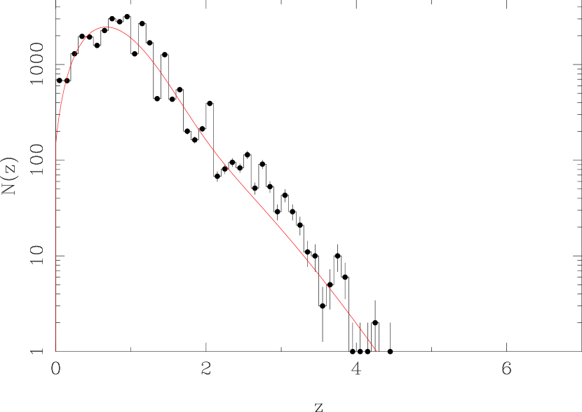
This prior can be extended to include magnitude dependence, , as done by Benítez (2000). We fit the functional form in Eq. 11 to the photo- catalog from Ilbert et al. (2009) in a number of -band magnitude bins. A sample fit is shown in Fig. 1 and the fitted parameters are summarized in Table 1. We note that one of the most popular codes bpz applies a template-dependent prior444 This template-dependent prior constrains relative fractions of galaxy populations (e.g., quiescent vs. star forming) as a function of redshift. Therefore, a care is needed when it is used for galaxy population studies. , but we assume that this prior is independent of templates.
| -mag range | |||
|---|---|---|---|
| 17.0–18.0 | 2.76 | 0.00 | 0.20 |
| 18.0–19.0 | 2.89 | 0.10 | 0.26 |
| 19.0–21.0 | 3.06 | 0.30 | 0.34 |
| 21.0–21.5 | 2.32 | 0.00 | 0.53 |
| 21.5–20.0 | 2.30 | 0.00 | 0.59 |
| 20.0–22.0 | 2.26 | 0.00 | 0.44 |
| 22.0–22.5 | 2.16 | 0.01 | 0.64 |
| 22.5–23.0 | 2.07 | 0.06 | 0.69 |
| 23.0–23.5 | 1.72 | 0.30 | 0.74 |
| 23.0–24.0 | 1.82 | 0.15 | 0.71 |
| 24.0–24.5 | 1.32 | 0.01 | 0.82 |
| 24.5–25.0 | 1.33 | 0.01 | 0.88 |
4.3.
There is a well-known correlation between SFR and stellar mass (e.g., Daddi et al. 2007; Elbaz et al. 2007; Wuyts et al. 2011b; Whitaker et al. 2012). This relation has been extensively studied across redshifts and we use it as a priori knowledge to constrain the model templates. The relation between SFR and stellar mass is not quite linear, but for simplicity, we assume a linear correlation between SFR and stellar mass ;
| (12) |
where
| (13) |
At , a typical SFR of a star forming galaxy with is and SFR at fixed mass increases at higher redshifts such that SFR is 10 times larger at . At higher redshifts, there is currently no consensus about the evolution of the star formation sequence. González et al. (2010) suggested that the evolution of sSFR (which is proportional to SFR at fixed mass) flattens out at , while Stark et al. (2013) hinted at a gradual increase at higher redshifts. We assume a gradual increase shown in Stark et al. (2013) with a redshift dependence of . We have confirmed that there is no strong effect on photo- accuracies if we assume no evolution at for the photo- tests performed in Section 6.
While star forming galaxies show a strong correlation between SFR and stellar mass, quiescent galaxies are off from that relation. We define a sequence for quiescent galaxies as the star forming sequence offset by dex. SED fitting does not reproduce SFRs at very low SFRs (Pacifici et al., 2012) and we find that this form works well after some experiments. SFRs can numerically be very small (e.g., ) and SFRs lower than dex from the star forming sequence are forced to be dex just for computational reasons.
Putting all this together, we assume that galaxies exhibit the two distinct sequences formed by star forming and quiescent galaxies and a probability of finding a galaxy with a star formation rate of SFR with a given stellar mass at redshift can be expressed as a sum of two Gaussians:
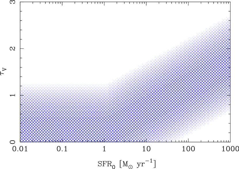
where is the mean SFR for a star forming galaxy at redshift and with stellar mass defined in Equation (12). We assume the relative fraction between the two populations is 1:1 at all redshifts to be conservative. and are the dispersions in each of the star forming and quiescent sequence. Here we take dex and dex. The observed scatter of the sequence may be smaller (e.g., 0.2 dex; Daddi et al. 2007), but starbursting galaxies are often located off from the sequence (Rodighiero et al., 2011) and we choose to assume a slightly large scatter. As for the quiescent sequence, low SFRs are difficult to measure from SEDs (Pacifici et al., 2012) and we adopt a large scatter. But, we should emphasize that photo- accuracies are not very sensitive to the choice of the scatters within reasonable ranges. Fig. 2 schematically illustrates this prior.

4.4.
An amount of attenuation is known to positively correlate with SFR as well as stellar mass (e.g., Hopkins et al. 2003; Garn & Best 2010). This fact has often been employed in photo- computations in the literature. E.g., Fontana et al. (2004) limited the attenuation to for low-SFR galaxies with , and Ilbert et al. (2009) did not apply extinction to their quiescent templates. Here, we formulate the relationship and implement it as a prior.
Sobral et al. (2012) suggested that the relationship between attenuation and stellar mass seems to remain unchanged out to . One might use this interesting relation as a prior, but the problem is that the relation is actually bimodal — at a given stellar mass, there are star forming and quiescent populations and only the former suffers from attenuation. To avoid this bimodality, we use the redshift-dependent SFR-attenuation relation555 The redshift independence of the mass-attenuation relation might appear odd at a first glance given the evolving relationship between SFR and stellar mass discussed above. The evolving SFR-mass relation seems to be compensated by the evolving SFR-attenuation relation, making the mass-attenuation independent of redshift. . We define an evolution corrected SFR as
| (15) |
where is defined in Eq. 12 and is used to eliminate the redshift dependence of the SFR-attenuation relation here. A factor of 100 is motivated to set the threshold SFR above which correlates with SFR to unity. We adopt a Gaussian form for this prior:
| (16) |
where
| (17) |
If a galaxy has a low SFR with its normalized SFR less than unity, the mean attenuation is fixed to a small value of 0.2. This non-zero value is adopted in order to leave room to compensate for metallicity variations. But, we have confirmed that photo- accuracies do not significantly change if we set it to zero. For the same reason, we adopt a relatively large of 0.5. The threshold is equivalent to SFR= at and is motivated by Garn & Best (2010). At higher SFRs, the mean attenuation increases with SFR. The adopted functional form reproduces the observation by Garn & Best (2010). The prior is schematically illustrated in Fig. 3.
We should note that the attenuation that Garn & Best (2010) measured is for H, which is known to suffer from a larger attenuation than the stellar continuum (Calzetti, 1997). The parameter in our models defines attenuation for stellar continuum and thus the mean attenuation assumed above should have been smaller by about a factor of 2. However, we find that the shallower relation results in poorer photo- accuracies. We speculate that this is due to a combined effect of (a) assumption of solar metallicity for all models and (b) dependence of attenuation curve on SFRs. As mentioned above, there is degeneracy between metallicity, age, and attenuation. We fix the metallicity to solar and let age and attenuation vary to compensate for the metallicity variation in real galaxies, which may affect the SFR-attenuation relation. Also, as discussed by Ilbert et al. (2009), the attenuation curve may be dependent on SFR, which also affects the relation. This is obviously an area where further work is needed.
4.5.
It is known, from experience, that templates with very young ages often give poor redshift accuracies and/or inaccurate physical properties (e.g., Fontana et al. 2004; Pozzetti et al. 2007; Tanaka et al. 2010; Wuyts et al. 2011a). This is primarily due to degeneracy introduced by these young templates; young templates all look similar regardless of their star formation timescales and they look similar even to older templates with long star formation timescales when only a small number of filters are available. All this is because the overall spectrum is dominated by young stars. Very young templates and/or templates with short are often manually excluded to reduce the degeneracy in the literature. Rather than manually removing them from the library, we prefer to put it on a more physical ground.
A crude, time-averaged mean star formation rate of a template can be given by
| (18) |
This is not strictly a mean SFR because the stellar mass-loss is not accounted for but is a reasonable proxy. Except for starbursting galaxies, steady-state star forming galaxies (i.e., those on the star formation sequence) have SFRs of up to a few hundred . Those are the most massive galaxies whose stellar mass (or equivalently SFR here) function follows an exponential form. Motivated by this, we assume a function of
| (19) |
This form gives a low probability to young templates and is effectively similar to the hard-cut priors adopted in the previous studies. A notable difference is that this form is more effective for more massive galaxies; a massive galaxy with young age has a low probability, while a low-mass galaxy with the same age has a high probability. This makes sense because low-mass galaxies are expected to be younger than massive galaxies. Another difference is that the characteristic SFR evolves with redshift in an observationally motivated way. This prior is schematically shown in Fig. 4.

4.6. Probability distribution function
The code produces a redshift PDF and the full PDF information should be used for any science analysis. But, it may be useful to make a point estimate for each object for certain purposes. A PDF of a galaxy can be quite complex and one faces a question of how to make such a point estimate. The most popular ways include: (1) peak of the PDF, (2) weighted mean, and (3) the median of the PDF. The definition of the first one is obvious. The latter two are defined as
| (20) |
and
| (21) |
where and are 0 and 7 in our case. After some experiments, we find that the median redshift works best. One might expect that the weighted redshift is a reasonable method because it uses the full PDF. But, a PDF often has multiple peaks and, depending on the relative probabilities of the peaks, the weighted redshift often lies in between the peaks. One can imagine a simple case in which there are two peaks with the same probability in a PDF, and the weighted redshift will be exactly in the middle of the peaks, where there is little probability.
The peak redshift is often adopted in the literature, but the median redshift works better. It is likely because the median redshift is a better tracer of the ’primary’ peak in PDF. Peaks in a PDF have different heights and widths and the peak with the largest integrated probability, not the peak probability, is more likely to be a correct redshift. This primary peak could be better identified by integrating the probability as done in the median redshift, not by locating the highest peak. One can explore an algorithm to directly identify the primary peak rather than taking the median of PDF, but for computational simplicity, we use the median redshifts in this paper.
5. Template error function
We use model templates generated with an SPS code. These model templates are subject to systematic uncertainties. Such uncertainties include deviation of star formation histories of real galaxies from the simple -model, ignorance of metallicity distribution, and errors in the stellar evolutionary track (which introduces an age-dependent systematics), etc. These systematic uncertainties cause mismatches between model SEDs and observed SEDs of galaxies. We use a template error function to crudely correct for such systematics. The template error function is first introduced by Brammer et al. (2008) and it is used to assign random uncertainties to templates. But, we extend it to include correction for systematic flux errors.
We define the template error function with two terms; systematic flux stretch and random flux uncertainty. The first term is a flux correction to model templates as a function of rest-frame wavelength and is meant to reduce mismatches with observed SEDs. This correction is typically small, of order a few percent, but can be as large as 10 per cent at some wavelengths. The second term assigns random uncertainties to the model fluxes to weight reliable parts of the SEDs, which is reasonable because model templates are often calibrated in the rest-frame optical and they can be more uncertain at other wavelengths.
A template error function can be easily coupled with zero-point offsets in photometric data in real analysis. In order to separate these two components, we first correct for systematic zero-point offsets by fitting spectroscopic objects located at low redshifts with their redshifts fixed to their spectroscopic redshifts. Given that the Sloan Digital Sky Survey (York et al., 2000) provides a large number of galaxies at over a wide area of the sky, we use objects located at and take the median of to estimate the zero-point offsets in a given filter. This process normally converges (i.e., offsets become less than 1%) after a few iterations. Note that no template error functions are applied in this process.
We then construct a template error function. For this, we need a large sample of spectroscopic redshifts over a wide range of redshift. This is fairly demanding and there are only a few deep fields that allow us to make error functions using spec-’s (e.g., Chandra Deep Field South as done in Tanaka et al. 2013a). A practical alternative would be to use very accurate photo-’s computed with many bands, which can be as accurate as , for this job. We use the photometry and the precise photometric redshift from Ilbert et al. (2009) to construct template error functions. We do not include medium-bands nor narrow-bands here because we are interested in flux errors smoothed over a typical bandwidth of broad-band filters. Narrow/Medium-band filters will give flux stretches on a finer wavelength scale. In other words, if one would like to apply a template error function to medium-band filters, that function has to be estimated separately from broad-bands.
We compute the systematic differences between the observed fluxes and the best-fit model fluxes using objects with precise photometric redshifts. Because objects spread over a range of redshift, we can effectively cover a wide range of rest-frame wavelength with the broad-band photometry alone. The median of at a given rest-frame wavelength is used to correct for the systematic template errors (1st term) and dispersion around the median is used as an uncertainty of the model templates at that rest-frame wavelength (2nd term). A typical photometric uncertainty in the observed data is subtracted off from the measured dispersion in order to derive intrinsic uncertainties in the models. In principle, one could apply such a correction to templates of a given spectral type. But, for now we simply make several redshift bins and apply a single “master” correction to all the templates in each bin in this paper.
Fig. 5 shows the template error functions in several redshift bins generated with the COSMOS data. The corrections are typically a few percent, but there are a few specific rest-frame wavelength ranges where the corrections can be as large as 10%. Maraston et al. (2009) showed that the observed color of passively evolving galaxies at is bluer by about 0.1 mag compared to models with an empirical stellar spectral library. Although a direct comparison with our template error functions cannot be made because we include star forming galaxies as well here, it is consistent that models are too red around the rest-frame 4000Å by about 10%. It is interesting to note that the template error functions evolve with redshift; the correction at increases towards . This has an implication for an age-dependent systematics in the SPS models, but a detailed study of it is beyond the scope of this paper. A template error function may provide an interesting way to address issues with SPS models using photometric data.

6. Improvements in photometric redshifts
We move on to demonstrate how the physical priors and template error functions improve photo-’s. We first describe the input photometric data and then define quantities to characterize photo-’s. After that, we present our photo-’s and discuss some of the outstanding issues.
A photo- accuracy is dependent on available filters and we focus on and photometry in the rest of the paper because these are the filter sets often available in large surveys; the HSC survey and DES observe in , CFHTLenS (which will be discussed in the next section) in , and LSST in . The -band photometry is not available in the public COSMOS data and thus the photo- accuracy we discuss below is a lower limit of these surveys. Another reason for this limited filter set is because priors play an important role. Many filters over a wide wavelength range provide a strong constraining power on SED shapes and redshifts and priors become less important (e.g., Ilbert et al. 2009 did not apply any priors because they had the 30-band photometry). Priors are more effective when less photometric information is available and the photometry is a good starting point to investigate how effective the physical priors introduced in Section 4 are.
6.1. Input photometric catalog
Obvious sources to characterize the accuracy of photo-’s are spectroscopic redshifts. There are a number of flux-limited/color-selected spectroscopic surveys in the literature. Some of the largest ones would include SDSS (York et al., 2000), GAMA (Driver et al., 2011), VVDS (Le Fèvre et al., 2005), VIPERS (Guzzo et al., 2013), PRIMUS (Coil et al., 2011), DEEP2 (Davis et al., 2003), and zCOSMOS (Lilly et al., 2007). The deepest of these is VVDS-UltraDeep, which is a flux limited survey at . It is a very unique source of absorption line redshifts of high redshift galaxies, which are mostly missed from shallower surveys. Unfortunately, however, even this deepest survey is still not deep enough to calibrate and validate photo-’s in the on-going/upcoming surveys, which reach or deeper. There is currently no spectroscopic sample that allows us to calibrate photo-’s down to this faint magnitude. Imaging goes deeper than spectroscopy.
A practical calibration ladder to reach faint magnitudes would be to use many-band photo-’s often available in deep fields. One notable example of this is photo-’s available in COSMOS (Ilbert et al., 2009), and in this section, we compare our photo-’s with the 30-band photo-’s down to . This is not as deep as we would like, but the public catalog does not contain fainter galaxies. Also, the COSMOS data are probably not deep enough to obtain good photo-’s at fainter magnitudes. The catalog is -selected and is suited to test our code in the context of large surveys, in which objects are often detected in the -band for weak-lensing science. There are more recent near-IR selected catalogs (Ilbert et al., 2013; Muzzin et al., 2013), but most of the above mentioned large surveys are optical surveys and we stick with the -selected catalog. We note that the effects of the physical priors and template error functions demonstrated below are not dependent on the detection filter. We show in the Appendix that they indeed significantly improve photo-’s for a -selected catalog.
We add 0.02 mag uncertainty in the quadrature to the cataloged uncertainties in Ilbert et al. (2009) because the uncertainties seem to be underestimated (reduced are often large for bright objects). This affects only bright galaxies for which uncertainties are smaller than mag. We also note that Ilbert et al. (2009) increased the uncertainties by a factor of 1.5 (which affects all galaxies) for their photo- analysis.
| case | physical priors | prior | template errfn | bias | ||||
|---|---|---|---|---|---|---|---|---|
| 1 | No | No | No | |||||
| 2 | Yes | No | No | |||||
| 3 | Yes | Yes | No | |||||
| 4 | Yes | Yes | Yes (w/o offset) | |||||
| 5 | Yes | Yes | Yes (w/ offset) | |||||
| 6 | No | Yes | Yes (w/ offset) |
6.2. Quantities to characterize photo-
There are a few standard quantities used to characterize photo- accuracies; bias, dispersion, and outlier rate. The definitions adopted in the literature are not always the same and we explicitly define them here for this work.
-
•
Bias: Photo-’s may systematically be off from spectroscopic redshifts and we call this systematic offset bias. We compute a systematic bias in by applying the biweight statistics (Beers et al., 1990). We iteratively apply 3 clipping for 3 times to reduce outliers.
-
•
Dispersion: In the literature, dispersion is often computed as
(22) where MAD is the median absolute deviation. Note that this definition does not account for the systematic bias. In addition to this conventional definition, we also measure the dispersion by accounting for the bias using the biweight statistics. We iteratively apply a clipping as done for bias to measure the dispersion around the central value. We denote the conventional dispersion and the biweight dispersion as and , respectively.
-
•
Outlier rate: The conventional definition is
(23) where outliers are defined as . Again, this definition does not account for the systematic bias. The threshold of 0.15 is an arbitrary value but is probably fine for photo-’s with several bands. It is clearly too large for those with many bands. Together with this conventional one, we also define outliers as those away from the central value (these and center are from biweight; see above). This is an arbitrary choice, but it is motivated to match reasonably well with the conventional one for several band photo-’s. We will denote the -based outlier fraction as and the conventional one as .
6.3. Photo- vs. spec-


Let us now demonstrate how the priors and template error function improve photo-. Table 2 summarizes the combination of the priors and template error functions and the resultant photo- accuracies discussed in this section. We shall emphasize that some of the many-band photo-’s that we compare with may be incorrect and thus we should not over-interpret the numbers discussed below in the absolute sense.
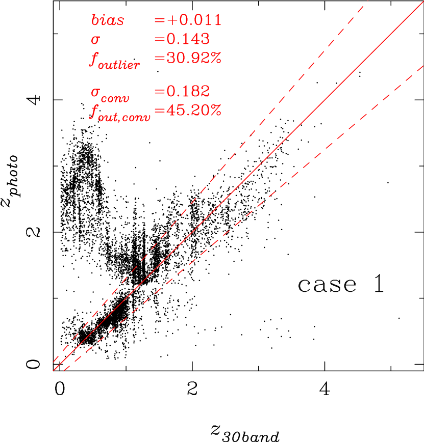
We start with the top-left panel of Fig. 6 (case 1), in which photo-’s computed without any of the physical priors and template error functions are compared with the high-accuracy photo-’s. As indicated in the plot, the scatter and outlier rate are both very high and the photo-’s are not very useful for any science applications. The mean bias is small (), but this is because a negative bias at is compensated by a positive bias at higher redshift by chance. The biggest failure mode is that a large fraction of low- galaxies up-scatter to high-. This is because the photometry probes redwards of the 4000Å break of these galaxies, where there is no prominent spectral feature. The blue continuum of low- star forming galaxies in the optical can be confused with blue UV continuum of galaxies at high redshifts, resulting in the up-scattered population. The overall poor photo- accuracy is the primary reason why SPS templates are not usually used for photo-’s and the two-step procedure with different templates is often adopted to estimate, e.g., stellar mass. We focus on a limited number of filters here, but SPS templates still give poorer accuracy than empirical templates even when more filters are used. E.g., Dahlen et al. (2013) carried out photo- tests with 14 filters for a number of codes and the typical performance of SPS-based codes is worse than that of empirical codes.
If we apply the physical priors (case 2 in Table 2 and Fig. 6), both the scatter and outlier rate significantly decrease. In particular, our primary failure mode of the up-scattered low- galaxies is suppressed. This is an important result and it proves the concept of our technique; the physical priors are indeed useful for improving photo-’s. Public photo- codes use a fixed set of SED templates regardless of redshift. The physical priors employed here effectively evolve the templates with redshift and the observed improvements suggest that the template evolution is actually important for photo-’s. We have not used information like sizes and morphologies here and there is clearly room for further improvements.
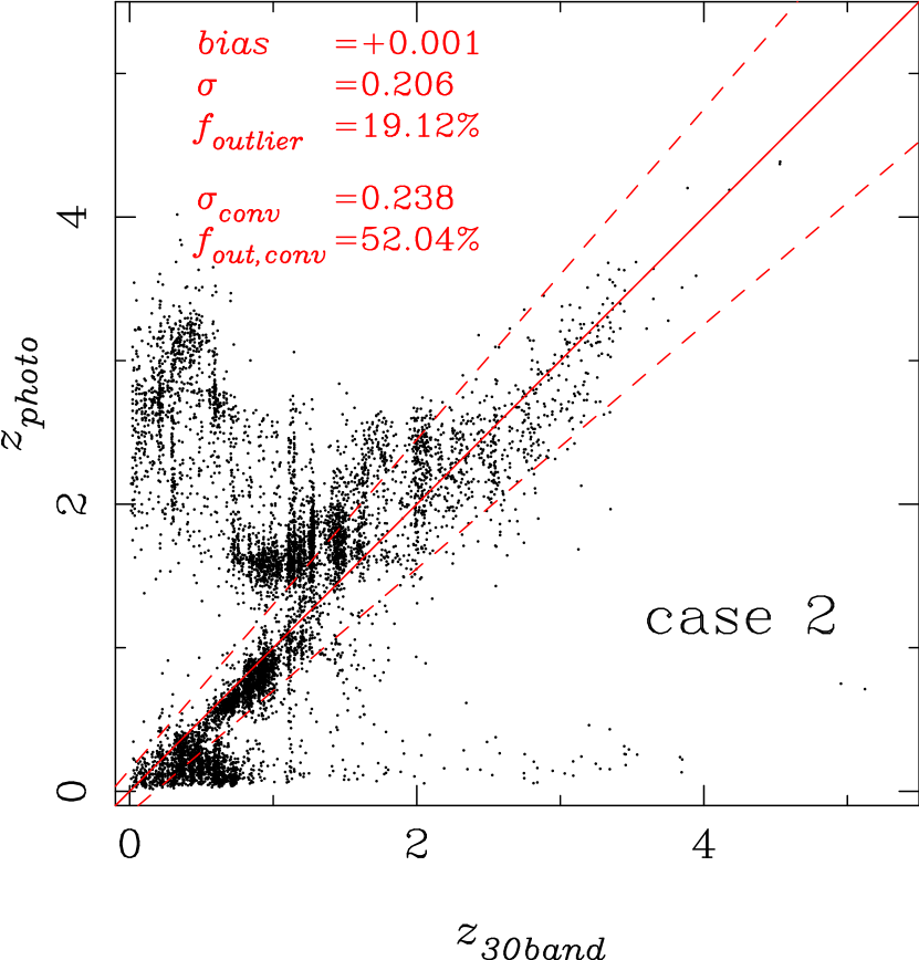
We then apply the standard prior (case 3). As expected, this prior is efficient in removing low- galaxies scattered out to high redshifts due to the degeneracy in the multi-color space discussed above. Both the overall scatter and outlier rate are reduced by the prior. But, the backside of it is that it is also effective in reducing correct photo-’s at . This is because those high redshift galaxies are rare and gives correspondingly small probabilities at high redshift. A preliminary analysis shows that this can be remedied by applying stronger physical priors with a less strong prior (e.g., one can introduce a ’floor’ in such that the minimum probability at a given redshift is some small fraction of the peak probability). This is also an area where further work is needed to achieve good photo-’s across the entire redshift range. We also should note that our prior is constructed from the Ilbert et al. (2009) catalog and we apply it to the same catalog here. We will need to extensively test the prior on a different catalog (see next section for comparisons with CFHTLenS).
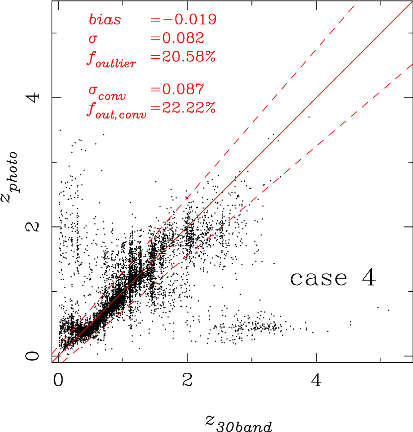
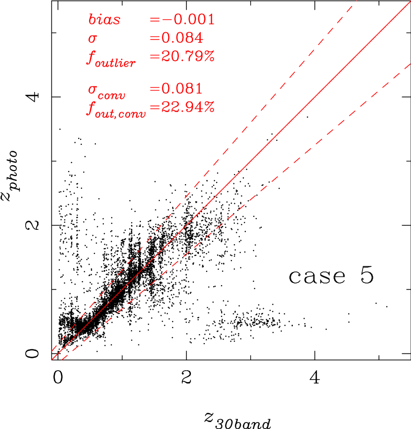
In addition to the priors, we apply the template error functions (case 4). The outlier rate () slightly increases, but this is due to the reduced (recall that outliers are defined as ). In fact, , which is based on the fixed outlier definition, is reduced. The overall accuracy is improved by the template error functions and this means that the systematic mismatches between the SPS templates and observed SEDs are in fact an issue in photo- and they have to be corrected. The implication here is not only for SPS models but for observed SED templates as well; a care must be taken when one applies observed SED templates collected at to high redshift galaxies because there will be systematic mismatches in the SEDs.
One may notice that there is a horizontal feature at both at low- and high-. Only faint () galaxies contribute to this feature. These faint galaxies have a wide and relatively flat PDF at , due to the large photometric uncertainties and to the limited filter set. For such PDF, the median redshift tends to cluster around . At higher redshift, more than 2 filters fall below the 4000Å break and we can achieve a reasonable accuracy until we get to , where the -band starts to fall below the Lyman break and again the photometric uncertainty becomes very large. As shown in the next section, the additional -band largely removes this feature.
Our overall photo- accuracy may not appear as good as those achieved in, e.g., DES (Sánchez et al., 2014). But, there are important differences in the depths, the redshift range considered, and analysis method used. Sánchez et al. (2014) studied galaxies with at and clipped 10% of the objects with large uncertainties, while we look at those with out to without any clipping. We will make a fair comparison with an external code in Section 7. Note that, for weak-lensing applications, the photo-’s in Fig. 6 are clearly not good enough and we do need to apply a clipping technique such as the one developed by Nishizawa et al. (2010) in order to reduce outliers.
6.4. Bias
There is an issue with our photo- case 4, which is that the photo-’s are biased low, bias=. This is illustrated in Fig. 7, in which the bias is plotted as a function of -band magnitude. This bias is a serious problem for weak-lensing cosmology, which requires mean redshift to be more accurate than 1 percent (e.g., Shirasaki & Yoshida 2014).
Interestingly, this systematic offset has already been observed by Dahlen et al. (2013), who analyzed deep HST data with several photo- codes. As shown in their Fig. 4, it is quite striking that most of the codes (even for the same code with different setups) show the same systematic offset of . Interestingly, the photo- comparisons by Sánchez et al. (2014) seem to suggest that machine-learning techniques do not show such an offset. It may be that a negative bias is a common problem in the SED-based photo- techniques. We find that the amount of the offset is dependent on the available data; if we use all the 30-band photometry in COSMOS, the bias is essentially zero (in fact, Ilbert et al. 2009 observed no bias), but the bias increases with decreasing the number of filters.
The negative bias has been observed but its origin has not been discussed in the literature. We have carefully looked into this issue, but we have not identified the root cause of the bias yet. We find that the prior introduces a negative bias, but it does not give a full account of the observed bias. We also find that the physical priors do not introduce a strong bias (see case 6 discussed below). The fact that public photo- codes that do not use physical priors also show a negative bias supports this finding. Just for now, we employ an ad-hoc correction to reduce the bias. Because we know we tend to underestimate redshifts by 0.02, we construct the template error functions with redshifts fixed to . The error functions constructed at offset redshifts reduce the bias as shown in Table 2, Figs. 6 and 7 (case 5), although they slightly increase the outlier rate. The bias is not completely gone as shown in Fig. 7 and further calibrations may be needed. We emphasize again that the negative bias is not a specific problem to our code, but a common problem.
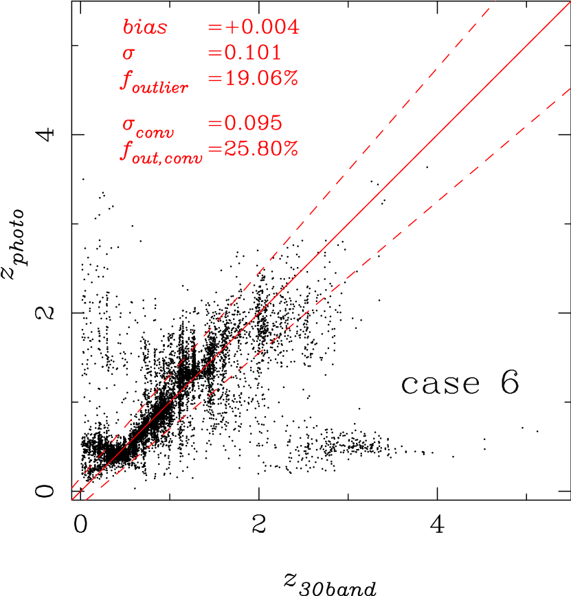
Finally, as the last proof of the effects of the physical priors, we show that photo-’s still improve even when they are applied after all the other corrections. Case 6 in Fig. 6 and Table 2 shows photo-s computed without the physical priors. A comparison with case 5 shows that the physical priors are indeed effective in reducing the outliers and dispersion even when they are added at the end. Based on all the above results, we conclude that the physical priors improve photo-’s. As a further illustration of the physical priors, we show how photo-’s change if we change the prior parameters in the Appendix.

6.5. Accuracy of P(z)
An important quality control of photo- is to assess the accuracy of PDF. It is difficult to estimate how accurate individual PDFs are, but the PDF accuracy can be addressed statistically. We compute fractions of objects that have photo-’s consistent with the 30-band photo-’s within 68 and 95 percentile intervals. If the PDFs are perfect, the fractions should be 68 and 95%. Deviations from these numbers are a manifestation of incorrect PDF.
In case 5, we find that 61% and 92% of objects have consistent photo-’s within 68 and 95 percentile intervals, respectively. It appears that our uncertainty estimates are slightly underestimated. Dahlen et al. (2013) observed a similar trend for a number of codes (see their Table 5). This seems to be another common problem in SED-based photo- codes. Catastrophic outliers probably contribute to the problem here and the reduction of those outliers will help. A careful construction of the template error functions will be useful too (recall that these functions include template uncertainties and thus are able to control photo- uncertainties). But, we do not perform further calibrations at this point because is strongly dependent on the accuracy of photometric uncertainties, which is not always straightforward to precisely measure. The fact that Ilbert et al. (2009) increased the flux uncertainty in the catalog by a factor of 1.5 does not seem to imply that the uncertainties are precisely measured. We also find that reduced of bright objects is often too large if we do not add a 0.02 mag uncertainty in the quadrature. We defer further work on to our future paper.
6.6. Brief summary
We have demonstrated that the physical priors and template error functions improve photo-’s. There are still issues left (e.g., understanding the root cause of the negative bias) and there is still room for improvements (e.g., priors on size and morphology), but the concept of the physical priors is proven to be useful. This is an important result. We are now motivated to compare our code with an external code to characterize how well our code works in the following sections.
7. Comparison with CFHTLenS
In this section, we compare our code with an external, publicly available code. We do not run an external code by ourselves in order to avoid any human biases (e.g., one may not fully calibrate an external code to make his/her own code work better). Instead, we use those from CFHTLenS (Heymans et al., 2012), which have been carefully computed by Hildebrandt et al. (2012) with one of the most popular public codes bpz (Benítez, 2000), to make a fair comparison.
7.1. Data
The photometric redshift in CFHTLenS is based on data from the CFHT Legacy Survey. The photometric data are obtained with MegaCam under good seeing conditions. We have retrieved the photometric data from the CFHTLenS database (Erben et al., 2013). CFHTLenS does not overlap with COSMOS and we here use spectroscopic redshifts from VVDS, not high-quality photo-’s as done in the previous section. We focus on two VVDS layers: VVDS-Deep and VVDS-UltraDeep, which are flux-limited to and to , respectively (Le Fevre et al., 2013). The surveys are performed with VIMOS on VLT with different instrumental setups, resulting in different redshift coverages. We discuss them separately. We select secure spectroscopic redshifts with flags 3 and 4 from these surveys and then cross-match them with the photometric objects from CFHTLenS within 1 arcsec. In total, we have 3,522 and 450 objects for VVDS-Deep and UltraDeep, respectively.
7.2. Comparison with bpz
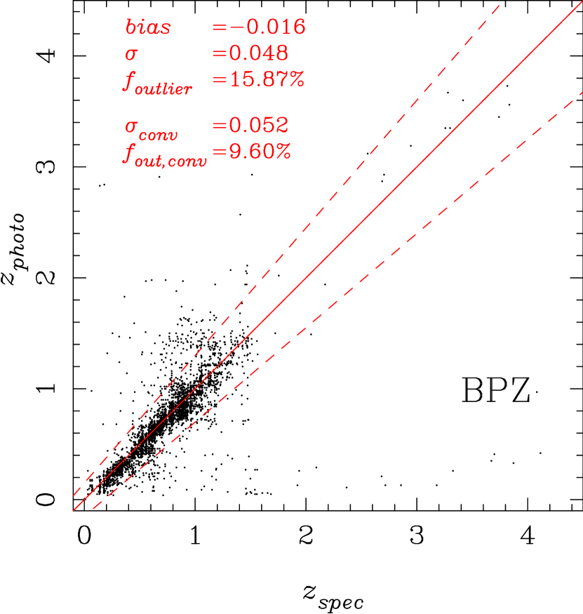
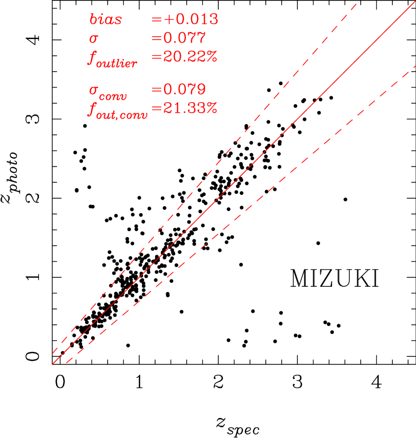
Let us start with VVDS-Deep shown in Fig. 8. The two codes perform similarly well; mizuki shows a higher outlier rate but with a slightly smaller scatter. The failure mode of mizuki is that a fraction of low- objects up-scatter to high-. Such failures are fewer in bpz. An interesting point here is that bpz has a small negative bias of . This negative bias again might be a common issue for SED fitting (see discussion in the previous section). On the other hand, mizuki’s bias is only +0.003 thanks to the template error function.
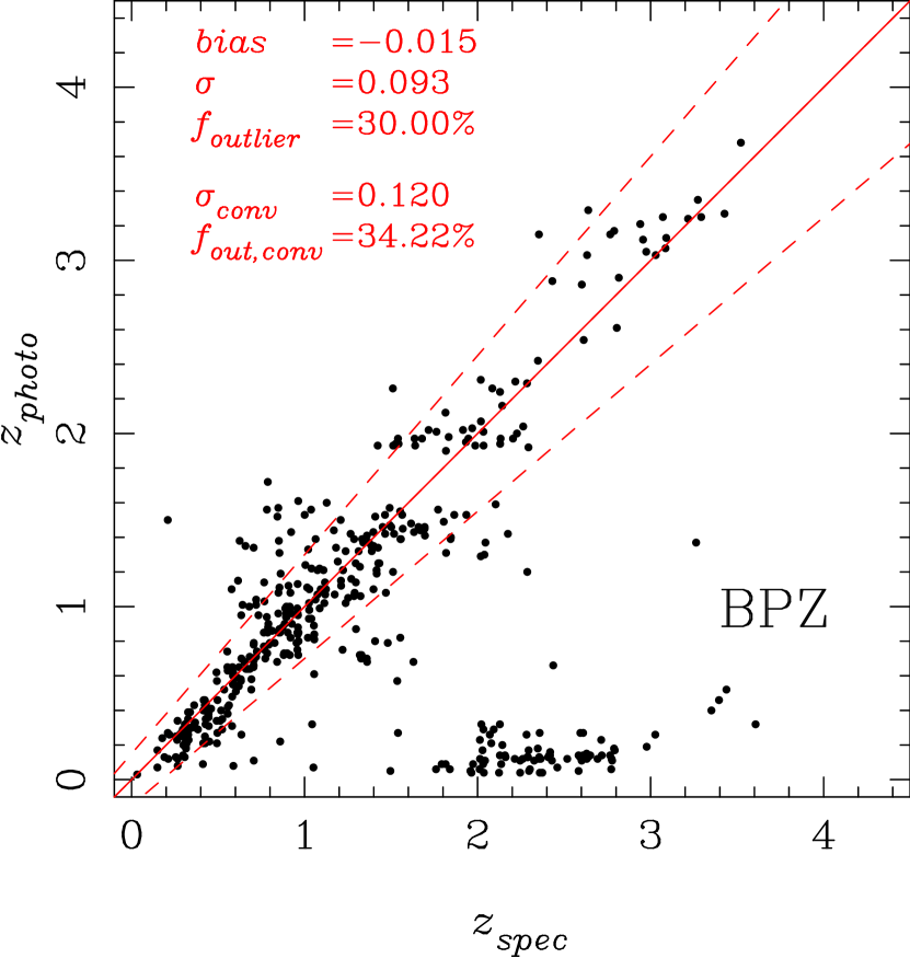
Turning to VVDS-UltraDeep in Fig. 9, there are objects all the way out to . Although the instrumental redshift selection function is probably not completely uniform, VVDS-UltraDeep is less biased compared to VVDS-Deep thanks to the very long integration time and a wider wavelength coverage. We find that bpz tends to give very low to galaxies at , which likely comes from the confusion between the Lyman break and the 4000Å break. It might be that the priors adopted in the code strongly prefer the low- solution, resulting in the down-scattered population. On the other hand, mizuki does not show such a strong failure and the numbers of outliers at low- and high- are about the same, suggesting the priors are about right.
In summary, mizuki is at least as good as bpz and possibly better at faint magnitudes and at high redshifts. The physical priors work well and the template error functions keep the bias smaller than that of bpz. While further calibrations may be needed, mizuki is already a powerful tool to infer photometric redshifts.

8. Biases in physical properties of galaxies
Physical properties and redshifts are very often inferred using different templates in the literature; one first uses empirical templates, PCA-based templates, or numerical techniques to compute redshift because they deliver better redshifts than SPS templates. Then, one switches to SPS templates to infer physical properties at the best-fit photo-. This is not a self-consistent way to infer them because different template sets may give different and the spectral shape and redshift are partially degenerate. Our code delivers good photo- accuracy and we can compute physical properties in a self-consistent manner. As of this writing, the code computes , , marginalized over all the other parameters.
We use the template error functions to remove small systematics in the SPS templates. Also, we apply the priors on physical properties. They may affect the inferred properties. In this section, we quantify biases in the inferred properties and show that they are well within the systematics of the SPS models that are inherent in any physical property estimates based on the SED fitting. In general, the recovery accuracy of physical properties is dependent on redshift accuracy, filter set (and depths), and details of the SED fitting technique. We have demonstrated in the previous sections that the template error functions and physical priors improve photo-. Also, intensive work on the recovery accuracy for a number of filter combination is already done by Pforr et al. (2012). For these reasons, we fix redshifts and assume only 2 representative filter sets in order to make useful comparisons focused on the fitting technique.
In the following, we make two comparisons: internal comparison and external comparison. The first one is to use our code with and without the template error functions and physical priors to quantify differences in the inferred properties. The 2nd one is to compare with a public SED fitting code with identical assumptions in the SPS models. As mentioned earlier, one should use the full PDFs of the physical properties for science analyses, but it is nevertheless useful to make point estimates. We take the median of PDF as done for redshift (see Eq. 21).
8.1. Data
For the purpose of the section, we need a public multi-wavelength catalog with physical property estimates. NEWFIRM medium band survey (NMBS; van Dokkum et al. 2009) is a good resource for this. NMBS achieved one of the most accurate photometric redshifts to date thanks to the large number of broad-band and medium-band photometry. This also allows reliable measurements of physical properties of galaxies. NMBS presents two catalogs: one in COSMOS and the other in AEGIS. We use the COSMOS catalog here because it includes medium-band data in the optical and is better than the other one (Whitaker et al., 2011). We take the photometry and photo-’s from the catalog for the analysis in the following section.
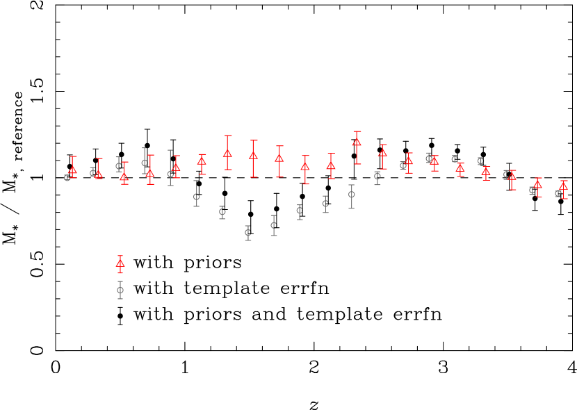
8.2. Internal comparison
First, we make an internal comparison. We compute stellar mass, SFR, and with and without the template error functions and the physical priors. The fits are performed at the NMBS photo-’s. Fig. 10 shows the differences in the inferred physical properties as a function of redshift. If only the priors are applied, there is only mild redshift dependence with a weak bias up to . The template error function introduces stronger redshift dependence, giving rise to bias at some redshifts. The bias for the priors and error functions combined is similar to that of the error function only case, which means that the overall bias is primarily due to the template error function. We know that SPS models do not perfectly reproduce the observed SEDs of galaxies, even for passively evolving galaxies (Maraston et al., 2009). Most authors nevertheless fit SPS models and use the one that is most similar to an observed SED to infer its physical properties. The % bias observed in Fig. 10 can be regarded as a level of the systematic uncertainty in this process. Fortunately, it is smaller than the overall systematic uncertainty inherent in the physical properties; e.g., Conroy et al. (2009) suggested that stellar mass measured at carries an uncertainty of about a factor of 2. While the bias introduced by the physical priors and template error functions should be kept in mind, it is unlikely to dominate the overall error budget.


8.3. External comparison
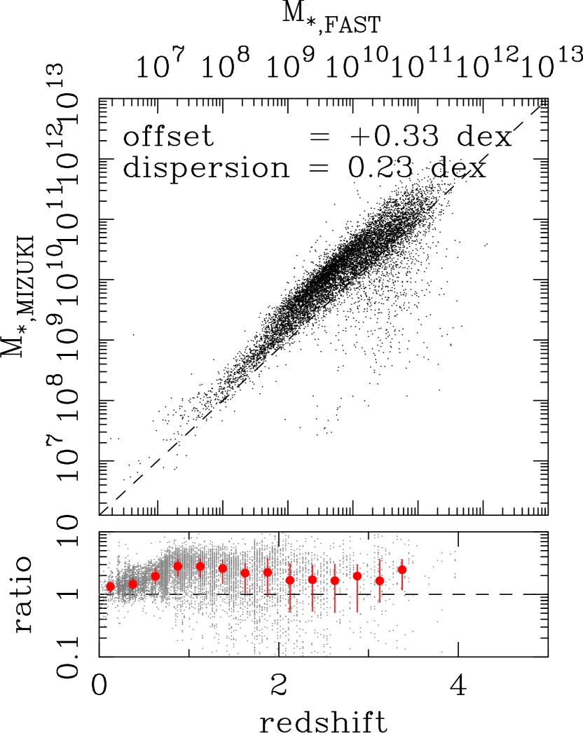
Next, we compare our code with fast (Kriek et al., 2009). fast is a code to infer physical properties of galaxies by fitting observed SEDs of galaxies with SPS models. Whitaker et al. (2011) applied the code to the NMBS data under identical assumptions to ours: Bruzual & Charlot (2003) SPS models with exponentially decaying star formation history, Chabrier IMF, Calzetti attenuation curve (Calzetti et al., 2000), and solar metallicity. fast is run with all the filters in the catalog, and a fair code-code comparison can be made if we use all the filters. But, we choose to primarily discuss the photometry in what follows in order to keep consistency with the previous sections and also to obtain a crude sense of how accurately we can infer the physical properties using optical data from large surveys. We summarize all of our results in Fig. 11 and Table 3. We discuss each physical property in turn.
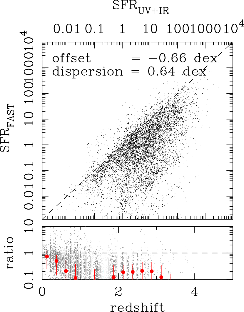
Stellar mass: On average, our stellar mass is about a factor of 2 higher than fast. This difference may not be too surprising because we use only 4 filters, while fast used more than 35 filters over a wider wavelength range. At , all of the filters fall below the 4000Å break and we lose an ability to constrain the stellar mass to luminosity ratio, resulting in the large bias and scatter at high redshifts. As shown in Table 3, the overall offset reduces to dex when we use all the available filters. Thus, the limited photometry, not the code or templates, is likely a primary cause of the offset. The typical statistical uncertainty in our stellar mass is 0.2-0.3 dex, even though we fix the redshift in the fits.
We note in passing that similar redshift dependence was observed by van Dokkum et al. (2014) in their comparison between the UltraVISTA and 3D-HST data. They used a large number of filters to infer stellar mass using fast, but they still observed a difference in stellar mass between the two data sets with a somewhat strong redshift dependence of dex. This seems to imply that, not only codes and templates, but data matter a lot.
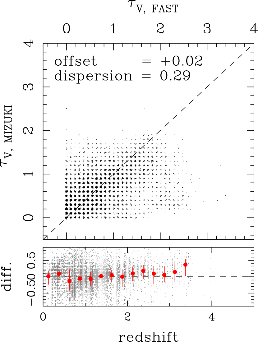
Dust attenuation: We find that our estimates are consistent with fast, although the dispersion is large . As discussed in Pacifici et al. (2012), we expect a large uncertainty in the inferred amount of attenuation from the broad-band photometry and we should first note that the attenuation inferred by fast is not the truth table here. With this caveat in mind, it is interesting that we do not observe a significant systematic difference at any redshifts. This is somewhat surprising because our photometry probe only the UV wavelengths at high redshifts. It is likely because the amount of attenuation is controlled well by the physical prior.
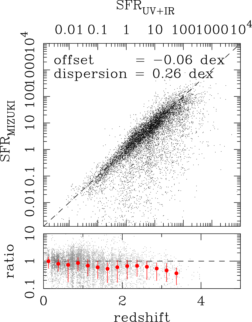
SFR: Whitaker et al. (2011) computed SFRs from the sum of the UV and IR luminosities under the reasonable assumption that absorbed UV photons are re-radiated thermally in the IR. The bottom-left panel of Fig. 11 compares with SFRs from fast based on the SED fitting. Assuming is a reasonable tracer of SFR, we find that fast tends to underestimate SFRs. At , SFRs from fast are lower by an order of magnitude. In contrast, mizuki estimates SFRs reasonably well as shown in the bottom-right panel. SFRs are slightly underestimated, but the overall agreement with is good and the dispersion (which is computed by clipping outliers as done in Section 6) is relatively small, a factor of . Interestingly, the offset increases if we include all the filters out to IR wavelengths (Table 3). One of the reasons for this would be our templates do not include thermal emission from warm dust yet.
Overall, physical properties inferred by mizuki agrees reasonably well with fast. There is a redshift-dependent offset in stellar mass, but it is likely due to the limited photometry. Amount of attenuation agrees well, and for SFR, mizuki works better than fast. Together with the good photo- accuracy demonstrated in the previous section, mizuki is a powerful tool to infer physical properties in a fully self-consistent manner.
| parameter | offset () | dispersion () | offset (all) | dispersion (all) |
|---|---|---|---|---|
| dex | dex | dex | dex | |
| — | — | dex | dex | |
| dex | dex | dex | dex |
9. Room for improvements
Throughout the paper, we have identified areas where further work is needed and there is clearly a large room for improvements in our technique. One of the ways forward would be to explore new priors. We have assumed solar metallicity in the SSP models, but given the recent substantial progress in the field, we could introduce a mass-metallicity prior. The size and morphology information has not been fully exploited in the literature (Wray & Gunn 2008 may be a notable exception) and the size-mass and morphology-mass (or SFR) priors would be interesting to explore. Surface brightness might be useful, too (Stabenau et al., 2008).
We also need to improve our templates. We have limited ourselves to optical data in this paper, but multi-wavelength data sets are often available in deep fields. One urgent improvement would be to include thermal emission from warm dust. Because we know the amount of attenuation and SFR for each template, we can add a model of thermal emission to the stellar SED based on the energy conservation (e.g., da Cunha et al. 2008). In addition to galaxies, we are also interested in stars and QSOs. We are making progress in QSO and stellar models as well as priors for them and we defer detailed discussions on them to our future paper.
Finally, speed. The current speed of the code is about 2 objects per second, which is too slow to be applied to survey data. The code can be optimized further and the same is true for templates; we find that 20-30% of the templates generated in Section 3 never give good fits to the observed SEDs of galaxies. We can safely remove those templates from the library, which will make the code faster. We aim to address these issues in our future work.
10. Summary
We have presented a proof-of-concept analysis of photometric redshifts with Bayesian priors on physical properties of galaxies such as SFR, stellar mass and dust attenuation. The priors are not fully optimized yet, but we have shown that the priors improve photometric redshifts significantly. Furthermore, template error functions, which are intended to correct for systematic flux errors as well as to assign random uncertainties to model templates, also improve photometric redshifts. We have compared our code with bpz, which is one of the most popular photo- codes, and shown that mizuki performs similarly well at bright magnitudes and it works better at faint magnitudes and at high redshifts.
One unique feature of the technique is that we can simultaneously infer redshifts and physical properties of galaxies in a fully self-consistent manner, unlike the two-step procedure with different templates often adopted in the literature. We have compared physical properties inferred by mizuki with those from fast under identical assumptions and confirmed that the inferred properties agree well, except for SFR, for which mizuki works significantly better. The priors and template error functions inevitably introduce a bias in the inferred physical properties of galaxies, but we have shown that it is small, . The bias is primarily due to mismatches between SPS SEDs and observed SEDs of galaxies and hence it is a problem common to all codes that use the Bruzual & Charlot (2003) model to infer physical properties.
Overall, mizuki is a powerful code to infer both redshifts and physical properties of galaxies. We have identified a number of areas where further work is needed throughout the paper. We will improve the code using data from the on-going large surveys such as the HSC survey. Once the code becomes mature enough, we will make the code available to the public.
We thank the HSC photo- working group, especially Atsushi Nishizawa and Jean Coupon, for useful discussions on many aspects of photo-, and the anonymous referee for useful comments. We acknowledge support by KAKENHI No. 23740144.
This work is based on observations obtained with MegaPrime/MegaCam, a joint project of CFHT and CEA/IRFU, at the Canada-France-Hawaii Telescope (CFHT) which is operated by the National Research Council (NRC) of Canada, the Institut National des Sciences de l’Univers of the Centre National de la Recherche Scientifique (CNRS) of France, and the University of Hawaii. This research used the facilities of the Canadian Astronomy Data Centre operated by the National Research Council of Canada with the support of the Canadian Space Agency. CFHTLenS data processing was made possible thanks to significant computing support from the NSERC Research Tools and Instruments grant program. This research uses data from the VIMOS VLT Deep Survey, obtained from the VVDS database operated by Cesam, Laboratoire d’Astrophysique de Marseille, France. This study makes use of data from the NEWFIRM Medium-Band Survey, a multi-wavelength survey conducted with the NEWFIRM instrument at the KPNO, supported in part by the NSF and NASA.
Appendix A Effects of priors and template error functions on a -selected catalog


The physical priors and template error functions introduced in the paper do not in principle depend on which filter is used for object detections, but it is still important to explicitly show that they work for a catalog that is not -selected. For this, we use the NMBS catalog used in Section 8, in which the objects are detected in the -band. Fig. 12 shows photo-’s for case 1, 2, and 7 using the photometry. In case 7, only the physical priors and template error functions with offsets are applied (i.e., no prior). We do not show the cases that involve the prior because the prior is for the -band and thus it by construction does not work well for a -selected sample. The statistics are summarized in Table 4.
A comparison between case 1 and 2 clearly demonstrate that the priors work very well for the -selected catalog; the up-scattered population at low- is strongly suppressed and the overall scatter is reduced. In addition, the template error functions applied in case 7 further improve the accuracy. In particular, the bias is significantly reduced and there is no remaining systematic offset. Based on these results, we conclude that the physical priors and template error functions are effective regardless of the detection filter.
| case | physical priors | prior | template errfn | bias | ||||
|---|---|---|---|---|---|---|---|---|
| 1 | No | No | No | |||||
| 2 | Yes | No | No | |||||
| 7 | Yes | No | Yes (w/ offset) |
Appendix B Effects of applying ’wrong’ physical priors

Our physical priors are motivated by observations, but it would be instructive to show what happens if we change the prior parameters. As an illustrative example, we change defined in Eq. 13 by dex. What it effectively does is to shift the observed sequence of star forming galaxies downwards by dex in the SFR vs stellar mass prior defined in Section 4.3. It also changes the attenuation prior in Section 4.4 in the sense that the prior has larger attenuation than what is observed.
We run our code with these ’wrong’ priors on the same COSMOS catalog as in Section 6. Here, we keep the prior and template error functions unchanged. The resultant photo-’s for case 2 and 5 are shown in Fig. 13. Statistics for all the cases are summarized in Table 5. Case 1 and 6 do not use the physical priors, but their accuracies are reproduced from Table 2 for easy comparisons. It is clear that the wrong priors degrade photo-’s. The priors give underestimated photo-’s at and overestimated ones at . This degradation is expected because the priors give a large probability to objects that do not really exist in the universe. In fact, by comparing with case 5 and 6 in Table 5, it is better not to apply the wrong physical priors. The improvement delivered by our fiducial physical priors shown in Section 6.3 in turn suggests that thes fiducial priors are not far from optimal.
| case | physical priors | prior | template errfn | bias | ||||
|---|---|---|---|---|---|---|---|---|
| 1 | No | No | No | |||||
| 2 | Yes | No | No | |||||
| 3 | Yes | Yes | No | |||||
| 4 | Yes | Yes | Yes (w/o offset) | |||||
| 5 | Yes | Yes | Yes (w/ offset) | |||||
| 6 | No | Yes | Yes (w/ offset) |
References
- Arnouts et al. (1999) Arnouts, S., Cristiani, S., Moscardini, L., et al. 1999, MNRAS, 310, 540
- Baum (1962) Baum, W. A. 1962, Problems of Extra-Galactic Research, 15, 390
- Beers et al. (1990) Beers, T. C., Flynn, K., & Gebhardt, K. 1990, AJ, 100, 32
- Benítez (2000) Benítez, N. 2000, ApJ, 536, 571
- Brammer et al. (2008) Brammer, G. B., van Dokkum, P. G., & Coppi, P. 2008, ApJ, 686, 1503
- Bruzual & Charlot (2003) Bruzual, G., & Charlot, S. 2003, MNRAS, 344, 1000
- Calzetti (1997) Calzetti, D. 1997, American Institute of Physics Conference Series, 408, 403
- Calzetti et al. (2000) Calzetti, D., Armus, L., Bohlin, R. C., et al. 2000, ApJ, 533, 682
- Chabrier (2003) Chabrier, G. 2003, PASP, 115, 763
- Carrasco Kind & Brunner (2013) Carrasco Kind, M., & Brunner, R. J. 2013, MNRAS, 432, 1483
- Collister & Lahav (2004) Collister, A. A., & Lahav, O. 2004, PASP, 116, 345
- Coil et al. (2011) Coil, A. L., Blanton, M. R., Burles, S. M., et al. 2011, ApJ, 741, 8
- Conroy et al. (2009) Conroy, C., Gunn, J. E., & White, M. 2009, ApJ, 699, 486
- Conroy & Gunn (2010) Conroy, C., & Gunn, J. E. 2010, ApJ, 712, 833
- Connolly et al. (1995) Connolly, A. J., Csabai, I., Szalay, A. S., et al. 1995, AJ, 110, 2655
- da Cunha et al. (2008) da Cunha, E., Charlot, S., & Elbaz, D. 2008, MNRAS, 388, 1595
- Dahlen et al. (2013) Dahlen, T., Mobasher, B., Faber, S. M., et al. 2013, ApJ, 775, 93
- Daddi et al. (2007) Daddi, E., Dickinson, M., Morrison, G., et al. 2007, ApJ, 670, 156
- Davis et al. (2003) Davis, M., Faber, S. M., Newman, J., et al. 2003, Proc. SPIE, 4834, 161
- The Dark Energy Survey Collaboration (2005) The Dark Energy Survey Collaboration 2005, arXiv:astro-ph/0510346
- de Jong et al. (2013) de Jong, J. T. A., Kuijken, K., Applegate, D., et al. 2013, The Messenger, 154, 44
- de Putter et al. (2014) de Putter, R., Doré, O., & Das, S. 2014, ApJ, 780, 185
- Driver et al. (2011) Driver, S. P., Hill, D. T., Kelvin, L. S., et al. 2011, MNRAS, 413, 971
- Elbaz et al. (2007) Elbaz, D., Daddi, E., Le Borgne, D., et al. 2007, A&A, 468, 33
- Erben et al. (2009) Erben, T., Hildebrandt, H., Lerchster, M., et al. 2009, A&A, 493, 1197
- Erben et al. (2013) Erben, T., Hildebrandt, H., Miller, L., et al. 2013, MNRAS, 433, 2545
- Feldmann et al. (2006) Feldmann, R., Carollo, C. M., Porciani, C., et al. 2006, MNRAS, 372, 565
- Fontana et al. (2004) Fontana, A., Pozzetti, L., Donnarumma, I., et al. 2004, A&A, 424, 23
- Garn & Best (2010) Garn, T., & Best, P. N. 2010, MNRAS, 409, 421
- González et al. (2010) González, V., Labbé, I., Bouwens, R. J., et al. 2010, ApJ, 713, 115
- Guzzo et al. (2013) Guzzo, L., Scodeggio, M., Garilli, B., et al. 2013, arXiv:1303.2623
- Henriques et al. (2012) Henriques, B. M. B., White, S. D. M., Lemson, G., et al. 2012, MNRAS, 421, 2904
- Heymans et al. (2012) Heymans, C., Van Waerbeke, L., Miller, L., et al. 2012, MNRAS, 427, 146
- Hildebrandt et al. (2010) Hildebrandt, H., Arnouts, S., Capak, P., et al. 2010, A&A, 523, A31
- Hildebrandt et al. (2012) Hildebrandt, H., Erben, T., Kuijken, K., et al. 2012, MNRAS, 421, 2355
- Hopkins et al. (2003) Hopkins, A. M., Miller, C. J., Nichol, R. C., et al. 2003, ApJ, 599, 971
- Hsieh & Yee (2014) Hsieh, B. C., & Yee, H. K. C. 2014, arXiv:1407.5151
- Ilbert et al. (2006) Ilbert, O., Arnouts, S., McCracken, H. J., et al. 2006, A&A, 457, 841
- Ilbert et al. (2009) Ilbert, O., Capak, P., Salvato, M., et al. 2009, ApJ, 690, 1236
- Ilbert et al. (2010) Ilbert, O., Salvato, M., Le Floc’h, E., et al. 2010, ApJ, 709, 644
- Ilbert et al. (2013) Ilbert, O., McCracken, H. J., Le Fevre, O., et al. 2013, arXiv:1301.3157
- Inoue (2011) Inoue, A. K. 2011, MNRAS, 415, 2920
- Ivezic et al. (2008) Ivezic, Z., Axelrod, T., Brandt, W. N., et al. 2008, Serbian Astronomical Journal, 176, 1
- Komatsu et al. (2011) Komatsu, E., Smith, K. M., Dunkley, J., et al. 2011, ApJS, 192, 18
- Kriek et al. (2009) Kriek, M., van Dokkum, P. G., Labbé, I., et al. 2009, ApJ, 700, 221
- Kriek et al. (2010) Kriek, M., Labbé, I., Conroy, C., et al. 2010, ApJ, 722, L64
- Lawrence et al. (2007) Lawrence, A., Warren, S. J., Almaini, O., et al. 2007, MNRAS, 379, 1599
- Le Fèvre et al. (2005) Le Fèvre, O., Vettolani, G., Garilli, B., et al. 2005, A&A, 439, 845
- Le Fevre et al. (2013) Le Fevre, O., Cassata, P., Cucciati, O., et al. 2013, arXiv:1307.6518
- Lilly et al. (2007) Lilly, S. J., Le Fèvre, O., Renzini, A., et al. 2007, ApJS, 172, 70
- Madau (1995) Madau, P. 1995, ApJ, 441, 18
- Maraston et al. (2009) Maraston, C., Strömbäck, G., Thomas, D., Wake, D. A., & Nichol, R. C. 2009, MNRAS, 394, L107
- Maraston et al. (2010) Maraston, C., Pforr, J., Renzini, A., et al. 2010, MNRAS, 407, 830
- McQuinn & White (2013) McQuinn, M., & White, M. 2013, MNRAS, 433, 2857
- Ménard et al. (2013) Ménard, B., Scranton, R., Schmidt, S., et al. 2013, arXiv:1303.4722
- Muzzin et al. (2013) Muzzin, A., Marchesini, D., Stefanon, M., et al. 2013, ApJS, 206, 8
- Newman (2008) Newman, J. A. 2008, ApJ, 684, 88
- Nishizawa et al. (2010) Nishizawa, A. J., Takada, M., Hamana, T., & Furusawa, H. 2010, ApJ, 718, 1252
- Pacifici et al. (2012) Pacifici, C., Charlot, S., Blaizot, J., & Brinchmann, J. 2012, MNRAS, 421, 2002
- Pforr et al. (2012) Pforr, J., Maraston, C., & Tonini, C. 2012, MNRAS, 422, 3285
- Pozzetti et al. (2007) Pozzetti, L., Bolzonella, M., Lamareille, F., et al. 2007, A&A, 474, 443
- Rodighiero et al. (2011) Rodighiero, G., Daddi, E., Baronchelli, I., et al. 2011, ApJ, 739, L40
- Sánchez et al. (2014) Sánchez, C., Carrasco Kind, M., Lin, H., et al. 2014, arXiv:1406.4407
- Santos et al. (2014) Santos, J. S., Altieri, B., Tanaka, M., et al. 2014, MNRAS, 438, 2565
- Schrabback et al. (2010) Schrabback, T., Hartlap, J., Joachimi, B., et al. 2010, A&A, 516, A63
- Schneider et al. (2006) Schneider, M., Knox, L., Zhan, H., & Connolly, A. 2006, ApJ, 651, 14
- Shirasaki & Yoshida (2014) Shirasaki, M., & Yoshida, N. 2014, ApJ, 786, 43
- Skrutskie et al. (2006) Skrutskie, M. F., Cutri, R. M., Stiening, R., et al. 2006, AJ, 131, 1163
- Sobral et al. (2012) Sobral, D., Best, P. N., Matsuda, Y., et al. 2012, MNRAS, 420, 1926
- Spergel et al. (2013) Spergel, D., Gehrels, N., Breckinridge, J., et al. 2013, arXiv:1305.5422
- Stabenau et al. (2008) Stabenau, H. F., Connolly, A., & Jain, B. 2008, MNRAS, 387, 1215
- Stark et al. (2013) Stark, D. P., Schenker, M. A., Ellis, R., et al. 2013, ApJ, 763, 129
- Tanaka et al. (2010) Tanaka, M., De Breuck, C., Venemans, B., & Kurk, J. 2010, A&A, 518, A18
- Tanaka et al. (2013a) Tanaka, M., Finoguenov, A., Mirkazemi, M., et al. 2013a, PASJ, 65, 17
- Tanaka et al. (2013b) Tanaka, M., Toft, S., Marchesini, D., et al. 2013b, ApJ, 772, 113
- van Dokkum et al. (2009) van Dokkum, P. G., Labbé, I., Marchesini, D., et al. 2009, PASP, 121, 2
- van Dokkum et al. (2014) van Dokkum, P., Bezanson, R., van der Wel, A., et al. 2014, arXiv:1404.4874
- Walcher et al. (2011) Walcher, J., Groves, B., Budavári, T., & Dale, D. 2011, Ap&SS, 331, 1
- Whitaker et al. (2011) Whitaker, K. E., Labbé, I., van Dokkum, P. G., et al. 2011, ApJ, 735, 86
- Whitaker et al. (2012) Whitaker, K. E., van Dokkum, P. G., Brammer, G., & Franx, M. 2012, ApJ, 754, L29
- Wray & Gunn (2008) Wray, J. J., & Gunn, J. E. 2008, ApJ, 678, 144
- Wuyts et al. (2011a) Wuyts, S., Förster Schreiber, N. M., Lutz, D., et al. 2011, ApJ, 738, 106
- Wuyts et al. (2011b) Wuyts, S., Förster Schreiber, N. M., van der Wel, A., et al. 2011, ApJ, 742, 96
- York et al. (2000) York, D. G., Adelman, J., Anderson, J. E., Jr., et al. 2000, AJ, 120, 1579
- Zibetti et al. (2013) Zibetti, S., Gallazzi, A., Charlot, S., Pierini, D., & Pasquali, A. 2013, MNRAS, 428, 1479