Fermi Large Area Telescope Third Source Catalog
Abstract
We present the third Fermi Large Area Telescope source catalog (3FGL) of sources in the 100 MeV–300 GeV range. Based on the first four years of science data from the Fermi Gamma-ray Space Telescope mission, it is the deepest yet in this energy range. Relative to the 2FGL catalog, the 3FGL catalog incorporates twice as much data as well as a number of analysis improvements, including improved calibrations at the event reconstruction level, an updated model for Galactic diffuse -ray emission, a refined procedure for source detection, and improved methods for associating LAT sources with potential counterparts at other wavelengths. The 3FGL catalog includes 3033 sources above significance, with source location regions, spectral properties, and monthly light curves for each. Of these, 78 are flagged as potentially being due to imperfections in the model for Galactic diffuse emission. Twenty-five sources are modeled explicitly as spatially extended, and overall 238 sources are considered as identified based on angular extent or correlated variability (periodic or otherwise) observed at other wavelengths. For 1010 sources we have not found plausible counterparts at other wavelengths. More than 1100 of the identified or associated sources are active galaxies of the blazar class; several other classes of non-blazar active galaxies are also represented in the 3FGL. Pulsars represent the largest Galactic source class. From source counts of Galactic sources we estimate the contribution of unresolved sources to the Galactic diffuse emission is 3% at 1 GeV.
1 Introduction
This paper presents a catalog of high-energy -ray sources detected in the first four years of the Fermi Gamma-ray Space Telescope mission by the Large Area Telescope (LAT). It is the successor to the LAT Bright Source List (hereafter 0FGL, Abdo et al., 2009d), the First Fermi LAT (1FGL, Abdo et al., 2010d) catalog, and the Second Fermi LAT (2FGL, Nolan et al., 2012) catalog, which were based on 3 months, 11 months, and 2 years of flight data, respectively. The 3FGL catalog both succeeds and complements the First Fermi LAT Catalog of Sources Above 10 GeV (1FHL, Ackermann et al., 2013a), which was based on 3 years of flight data but considered only sources detected above 10 GeV. The new 3FGL catalog is the deepest yet in the 100 MeV–300 GeV energy range. The result of a dedicated effort for studying the Active Galactic Nuclei (AGN) population in the 3FGL catalog is published in an accompanying paper (3LAC, Ackermann et al., 2015).
We have implemented a number of analysis refinements for the 3FGL catalog:
-
1.
Pass 7 reprocessed data111See http://fermi.gsfc.nasa.gov/ssc/data/analysis/documentation/Pass7REP_usage.html. are now used (§ 2.2). The principal difference relative to the original Pass 7 data used for 2FGL is improved angular resolution above 3 GeV. In addition, systematics of the instrument response functions (IRFs) are better characterized, and smaller.
-
2.
This catalog employs a new model of the diffuse Galactic and isotropic emissions, developed for the 3FGL analysis (§ 2.3). The model has improved fidelity to the observations, especially for regions where the diffuse emission cannot be described using a spatial template derived from observations at other wavelengths. In addition, the accuracy of the model is improved toward bright star-forming regions and at energies above 40 GeV generally. The development of this model is described in a separate publication (Casandjian & the Fermi LAT Collaboration, 2015).
-
3.
We explicitly model twenty-five sources as extended emission regions (§ 3.4), up from twelve in 2FGL. Each has an angular extent measured with LAT data. Taking into account the finite sizes of the sources allows for more accurate flux and spectrum measurements for the extended sources as well as for nearby point sources.
-
4.
We have further refined the method for characterizing and localizing source ‘seeds’ evaluated for inclusion in the catalog (§ 3.1). The improvements in this regard are most marked at low Galactic latitudes, where an iterative approach to finding seeds has improved the sensitivity of the catalog in the Galactic plane.
-
5.
For studying the associations of LAT sources with counterparts at other wavelengths, we have updated several of the catalogs used for counterpart searches, and correspondingly recalibrated the association procedure.
The exposure of the LAT is fairly uniform across the sky, but the brightness of the diffuse backgrounds, and hence the sensitivity for source detection, depends strongly on direction. As for previous LAT source catalogs, for the 3FGL catalog sources are included based on the statistical significance of their detection considered over the entire time period of the analysis. For this reason the 3FGL catalog is not a comprehensive catalog of transient -ray sources, however the catalog does include light curves on a monthly time scale for sources that meet the criteria for inclusion.
In § 2 we describe the LAT and the models for the diffuse backgrounds, celestial and otherwise. Section 3 describes how the catalog is constructed, with emphasis on what has changed since the analysis for the 2FGL catalog. The 3FGL catalog itself is presented in § 4, along with a comparison to previous LAT catalogs. We discuss associations and identifications in § 5 and Galactic source counts in § 6. The conclusions are presented in § 7. We provide appendices with technical details of the analysis and of the format of the electronic version of the catalog.
2 Instrument and Background
2.1 The Large Area Telescope
The LAT detects rays in the energy range 20 MeV to more than 300 GeV, measuring their arrival times, energies, and directions. The LAT is also an efficient detector of the intense background of charged particles from cosmic rays and trapped radiation at the orbit of the Fermi satellite. Accounting for rays lost in filtering charged particles from the data, the effective collecting area is 6500 cm2 at 1 GeV (for the P7REP_SOURCE_V15 event selection used here; see below). The live time is nearly 76%, limited primarily by interruptions of data taking when is passing through the South Atlantic Anomaly (13%) and readout dead-time fraction (9%). The field of view of the LAT is 2.4 sr at 1 GeV. The per-photon angular resolution (point-spread function, PSF, 68% containment) is 5 at 100 MeV, decreasing to at 1 GeV (averaged over the acceptance of the LAT), varying with energy approximately as and asymptoting at above 20 GeV. The tracking section of the LAT has 36 layers of silicon strip detectors interleaved with 16 layers of tungsten foil (12 thin layers, 0.03 radiation length, at the top or Front of the instrument, followed by 4 thick layers, 0.18 radiation length, in the Back section). The silicon strips track charged particles, and the tungsten foils facilitate conversion of rays to positron-electron pairs. Beneath the tracker is a calorimeter composed of an 8-layer array of CsI crystals (8.5 total radiation lengths) to determine the -ray energy. A segmented charged-particle anticoincidence detector (plastic scintillators read out by photomultiplier tubes) around the tracker is used to reject charged-particle background events. More information about the LAT is provided in Atwood et al. (2009), and the in-flight calibration of the LAT is described in Abdo et al. (2009g), Ackermann et al. (2012c), and Ackermann et al. (2012a).
2.2 The LAT Data
The data for the 3FGL catalog were taken during the period 2008 August 4 (15:43 UTC)–2012 July 31 (22:46 UTC) covering close to four years. They are the public data available from the Fermi Science Support Center (FSSC). Intervals around bright GRBs (080916C, 090510, 090902B, 090926A, 110731A; Ackermann et al., 2013b) were excised. Solar flares became relatively frequent in 2011–12 (close to solar maximum) and were excised as well whenever they were bright enough to be detected over a month at the level. Solar flares last much longer than GRBs, so we were attentive not to reject too much time. Since the -ray emission is localized on the Sun, we kept intervals during which the Sun was at least below the Earth limb222This selection in FTOOLS notation is ANGSEP(RA_SUN,DEC_SUN,RA_ZENITH,DEC_ZENITH) > 115. even during solar flares. The solar flares were detected over 3-hour intervals so the corresponding Good Time Intervals (GTI) are aligned to those 3-hour marks. Overall about two days were excised due to solar flares. In order to reduce the contamination from the -ray-bright Earth limb (§ 2.3.4), times when the rocking angle of the spacecraft was larger than 52°, and events with zenith angles larger than 100°, were excised as well. The precise time intervals corresponding to selected events are recorded in the GTI extension of the 3FGL catalog (FITS version, App. B).
The rocking angle remained set at after September 2009 (it was for about 80% of the time before that333See the LAT survey-mode history at http://fermi.gsfc.nasa.gov/ssc/observations/types/allsky/.). With the larger rocking angle the orbital plane is further off axis with the result that the survey is slightly non-uniform. The maximum exposure is reached at the North celestial pole. At 1 GeV it is 60% larger than the minimum exposure, which is reached at the celestial equator (Figure 1).

In parallel with accumulating new data, developments on the instrument analysis side (Bregeon et al., 2013) led to reprocessing all LAT data with new calibration constants, resulting in the Pass 7 reprocessed data that were used for 3FGL444Details about the performance of the LAT are available at
http://www.slac.stanford.edu/exp/glast/groups/canda/lat_Performance.htm.. The main advantage for the source catalog is that the reprocessing improved the PSF above 10 GeV by 30%, improving the localization of hard sources (§ 3.1). We used the Source class event selection.
The lower bound of the energy range was left at 100 MeV, but the upper bound was raised to 300 GeV as in the 1FHL catalog. This is because as the source-to-background ratio decreases, the sensitivity curve (Figure 18 of Abdo et al., 2010d, 1FGL) shifts to higher energies.
2.3 Model for the Diffuse Gamma-Ray Background
Models for the diffuse -ray backgrounds were updated for the 3FGL analysis, taking into account the new IRFs for Pass 7 reprocessed data and the improved statistics available with a 4-year data set, and also applying some refinements in the procedure for evaluating the models. The primary components of the diffuse backgrounds are the diffuse -ray emission of the Milky Way and the approximately isotropic background consisting of emission from sub-threshold celestial sources plus residual charged particles misclassified as rays. In addition, we treat the ‘passive’ emission of the Sun and Moon from cosmic-ray interactions with the solar atmosphere, solar radiation field, and the lunar lithosphere, as effectively a diffuse component, because the Sun and Moon move across the sky. The residual Earth limb emission after the zenith angle selection (§ 2.2) is also treated as effectively diffuse. Each component of the background model for the 3FGL analysis is described in more detail below.
2.3.1 Diffuse emission of the Milky Way
The diffuse -ray emission of the Milky Way originates in cosmic-ray interactions with interstellar gas and radiation. As for 2FGL, for any given energy the model is primarily a linear combination of template maps derived from CO and H i line survey data plus infrared maps of interstellar dust, which trace interstellar gas and in the model represent the -ray emission from pion decay and bremsstrahlung. In addition we include in the model a template representing the intensity of emission from inverse Compton scattering of cosmic-ray electrons on the interstellar radiation field. This component was calculated using the GALPROP code555See http://galprop.stanford.edu. (Moskalenko & Strong, 1998).
For the 3FGL analysis we have made several improvements relative to 2FGL in modeling the diffuse emission. The development of this new model is described by Casandjian & the Fermi LAT Collaboration (2015)666The model is available as gll_iem_v05_rev1.fit from the FSSC.. Here we briefly summarize the improvements. For 3FGL the representation of the gas traced uniquely by the infrared maps was improved in the vicinity of massive star-forming regions. The overall model was fit to the LAT data iteratively, taking into account a preliminary version of the 3FGL source list, for the energy range 50 MeV–50 GeV. Relative to the 2FGL model for Galactic diffuse emission, we have improved the extrapolation to lower and higher energies using the energy dependence of the -ray emissivity function. We developed a new procedure to account for the structured celestial -ray emission that could not be fit using templates derived from observations at other wavelengths. This residual component, also fit iteratively, was derived by deconvolving the residuals to take into account the effects of the PSF, filtering the result to reduce statistical fluctuations (removing structures on angular scales smaller than 2). The spectrum was modeled as inverse Compton emission from a population of cosmic-ray electrons with a spectral break at 965 MeV.
2.3.2 Isotropic background
The isotropic diffuse background was derived from all-sky fits of the four-year data set using the Galactic diffuse emission model described above and a preliminary version of the 3FGL source list. The diffuse background includes charged particles misclassified as rays. We implicitly assume that the acceptance for these residual charged particles is the same as for rays in treating these diffuse background components together. For the analysis we derived the contributions to the isotropic background separately for -converting and -converting events. They are available as iso_source_xxx_v05.txt from the FSSC, where xxx is front or back.
2.3.3 Solar and lunar template
The quiescent Sun and the Moon are fairly bright -ray sources (Abdo et al., 2011b, 2012b). The Sun moves in the ecliptic but the solar -ray emission is extended because of cosmic-ray interactions with the solar radiation field; detectable emission from inverse Compton scattering of cosmic-ray electrons on the radiation field of the Sun extends several degrees from the Sun (Abdo et al., 2011b). The Moon is not an extended source in this way but the lunar orbit is inclined somewhat relative to the ecliptic and the Moon moves through a larger fraction of the sky than the Sun. Averaged over time, the -ray emission from the Sun and Moon trace a region around the ecliptic. We used models of their observed emission together with calculations of their motions and of the exposure of the observations by the LAT to make templates for the equivalent diffuse component for the 3FGL analysis using (Johannesson et al., 2013). For the light curves (§ 3.6) we evaluated the equivalent diffuse components for the corresponding time intervals.
2.3.4 Residual Earth limb template
The limb of the Earth is an intense source of rays from cosmic-ray collisions with the upper atmosphere (Abdo et al., 2009a). At the 565 km altitude of the (nearly-circular) orbit of the LAT, the limb is 112 from the zenith. During survey-mode observations, which predominated in the first four years of the Fermi mission, the spacecraft was rocked toward the northern and southern orbital poles on alternate 90 minute orbits. With these attitudes, the edge of the LAT field of view closest to the orbital poles generally subtended part of the Earth limb. As described in § 2.2, we limited the data selection and exposure calculations to zenith angles less than 100. Because the Earth limb emission is so intense, and the tails of the LAT PSF are long (Ackermann et al., 2012a), a residual component of limb emission remained in the data. Over the course of a precession period of the orbit (53 d), the residual glow fills out large ‘caps’ around the celestial poles, with the angular radius determined by the sum of the orbital inclination () and the angular distance of the zenith angle limit from the orbital pole (10). Casandjian & the Fermi LAT Collaboration (2015) describe how the map and spectrum of the residual component were derived. The spectrum is well modeled as a steep power law in energy with index 4.25. This is steep enough that the residual Earth limb emission contributes significantly only below 300 MeV.
3 Construction of the Catalog
The procedure used to construct the 3FGL catalog has a number of improvements relative to what was implemented for the 2FGL catalog. In this section we review the procedure, with an emphasis on what is being done differently. The significances (§ 3.2), spectral parameters (§ 3.3) and fluxes (§ 3.5) of all catalog sources were obtained using the standard framework (Python analog of ) in the LAT Science Tools777See http://fermi.gsfc.nasa.gov/ssc/data/analysis/documentation/Cicerone/. (version v9r32p5). The localization procedure (§ 3.1), which relies on , provided the source positions, the starting point for the spectral fitting, and a comparison for estimating the reliability of the results (§ 3.7.4). Throughout the text we use the Test Statistic for quantifying how significantly a source emerges from the background, comparing the likelihood function with and without that source.
3.1 Detection and Localization
This section describes the generation of a list of candidate sources, with locations and initial spectral fits, for processing by the standard LAT science analysis tools, especially to compute the likelihood (§ 3.2). This initial stage uses instead (Kerr, 2010). Compared with the -based analysis described in § 3.2 to 3.7, it uses the same data, exposure, and IRFs, but the partitioning of the sky, the computation of the likelihood function, and its optimization, are independent. Since this version of the computation of the likelihood function is used for localization, it needs to represent a valid estimate of the probability of observing a point source with the assumed spectral function.
The process started with an initial set of sources from the 2FGL analysis; not just those reported in that catalog, but also including all candidates failing the significance threshold (i.e., with ). It also used the latest extended source list with 25 entries (§ 3.4), and the three-source representation of the Crab (§ 3.3). The same spectral models were considered for each source as in § 3.3, but the favored model (power law or curved) was not necessarily the same.
Many details of the processing were identical to the 2FGL procedure: using HEALPix888http://healpix.sourceforge.net. (Górski et al., 2005) with , to tile the sky, resulting in 1728 tiles of 25 deg2 area; optimizing spectral parameters for the sources within each tile, for the data in a cone of 5 radius about the center of the tile; and including the contributions of all sources within 10 of the center. The tiles are of course discrete, but the regions, which we refer to as RoIs, for Regions of Interest, are overlapping and not independent. The data were binned in energy (14 energy bands from 100 MeV to 316 GeV) and position, where the angular bin size (the bins also defined using HEALPix) was set to be small compared with the PSF for each energy, and event type. Separating the photons according to event type is important, especially for localization, since the -converting events have a factor of two narrower PSF core than the -converting events. Thus the parameter optimization was performed by maximizing the logarithm of the likelihood, expressed as a sum over each energy band and each of the two event types (, ). The fits for each RoI, maximizing the likelihood as a function of the free parameters, were performed independently. Correlations between sources in neighboring RoIs were then accounted for by iterating all 1728 fits until the changes in the log likelihoods for all RoIs were less than 10.
After a set of iterations had converged, then the localization procedure was applied, and source positions updated for a new set of iterations. At this stage, new sources were occasionally added using the residual procedure described below. The detection and initial localization process resulted in 4029 candidate point sources with .
New features that are discussed below include an assessment of the reliability of each spectral fit and of the model as a whole in each RoI, a different approach to the normalization of the Galactic diffuse background component, and a method to unweight the likelihood to account for the effect of potential systematic errors in the Galactic diffuse on source spectra.
3.1.1 Fit validation
An important criterion is that the spectral and spatial models for all sources are not only optimized, but that the predictions of the models are consistent with the data. Maximizing the likelihood as an estimator for spectral parameters and position is valid only if the likelihood, given a set of parameters, corresponds to the probability of observing the data. We have three measures.
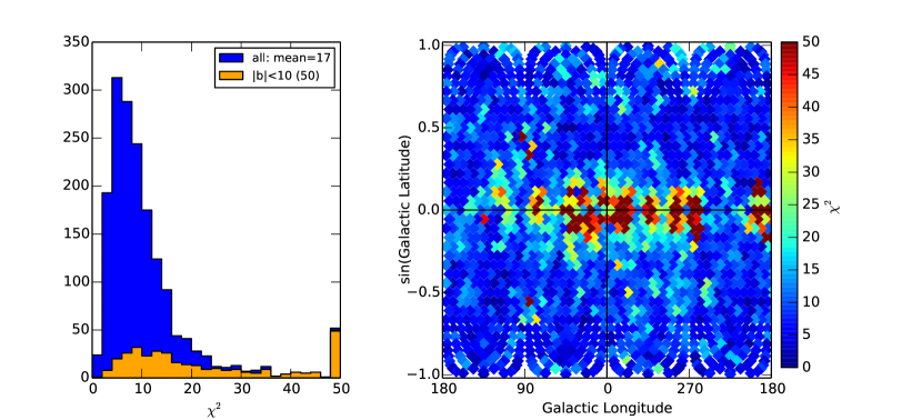
The first compares the number of counts in each energy band, combining and , for each of the 1728 regions, defining a -like measure as the sum of the squares of the deviations divided by the predicted number of counts. The number of counts is the expected variance for Poisson counting statistics. This measure is of course only a component of the likelihood, and depends only weakly on most of the point sources. That is, maximizing the likelihood does not necessarily minimize this quantity. But it is important to check the reliability of the diffuse model used, since this can distort the point source spectral fits. Figure 2 shows the distribution of that -like measure and its values as a function of location on the sky. The number of degrees of freedom is 14 (the number of energy bands) minus the effective number of variables. The fact that the distribution peaks at seems sensible. The 35 regions with indicate problems with the model. Most are close to the Galactic plane, indicating difficulty with the component representing the Galactic diffuse emission. The few at high latitudes could be due to missing sources or, for very strong sources, inadequacy of the simple spectral models that we use.
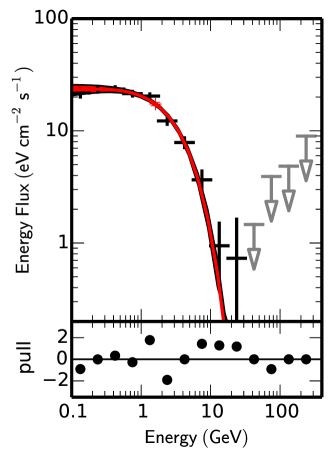
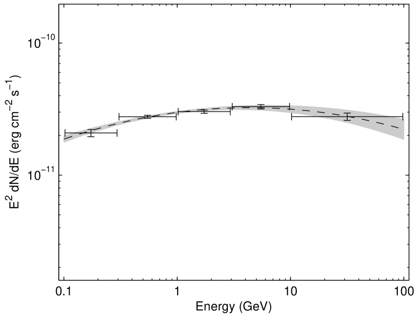
The second measure is a check that the spectral model for each source is consistent with the data. The likelihood associated with a source is the product of the likelihoods for that source for each energy band, including the contributions of nearby, overlapping sources, and the diffuse backgrounds. The correlations induced by those are only relevant for the lower energies, typically below 1 GeV. For this analysis, we keep these contributions fixed. We form the spectral fit quality as where the flux for each band is optimized independently in whereas the spectral model is applied in . The spectrum in Figure 3 illustrates the concept.
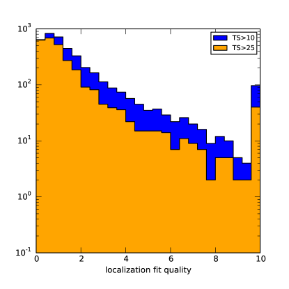
In Figure 4, we show the distribution of the spectral fit quality for all preliminary spectra, with separate plots for the three different spectral functions (§ 3.3): power law, log-normal, and power law with an exponential cutoff. The latter, applied almost exclusively to pulsars, is separated into sources in and out of the Galactic plane. It is seen that sources in the plane often have poorer fits. All are compared with an example distribution with 10 degrees of freedom. There are 14 bands, and two to four parameters, but the higher-energy bands often do not contribute, so the number of degrees of freedom is not well defined and we use 10 for illustration only.

Finally, the localization process fits the logarithm of the likelihood as a function of position to a quadratic form, and checks the consistency with a -like measure (§ 3.1.3).
3.1.2 Galactic diffuse normalization and unweighting
The model that we used for the Galactic diffuse background is a global fit using the data, as described in § 2.3. For an individual RoI however, we found that we needed to adjust the normalizations for each band to fit the data. For the relatively broad energy bands, four per decade, used in the fit we allow the normalization for each band to vary, effectively ignoring the spectral prediction of the diffuse component analysis. So, for each of the 1728 RoIs, and for each of the eight energy bands below 10 GeV, we measured a normalization factor, which applies to both and , by maximizing the likelihood with respect to it. A motivation for this procedure was that, for the lowest energy bands, it often improved the fit consistencies of the spectral models of the sources in the same RoI.
While the precision of the determination of the average contribution from the Galactic diffuse for an energy band is subject to only the statistics of the number of photons, the value of the Galactic diffuse intensity at the location of each source, that is, the angular distribution of the intensity, is subject to an additional systematic error. Since this intensity is strongly correlated with the measurement of the flux from the source itself, and the correlation can be very significant for weak sources, we have adopted an ad hoc, but conservative procedure to account for the additional uncertainty by increasing the width of the log likelihood distribution from each energy band according to how sensitive it is to the Galactic diffuse contribution. This is accomplished by dividing the log likelihood by max(1,/1000) where is the predicted number of Galactic diffuse photons in the RoI. This has the effect of limiting the precision to the statistics of 1000 photons in the RoI and energy band, i.e. it unweights contributions from energy ranges for which the contribution from the diffuse component is relatively less well defined.
3.1.3 Localization
The position of each source was determined by maximizing the likelihood with respect to its position only. That is, all other parameters are kept fixed. The possibility that a shifted position would affect the spectral models or positions of nearby sources is accounted for by iteration. Ideally, the likelihood is the product of two Gaussians in two orthogonal angular variables. Thus the log likelihood is a quadratic form in any pair of angular variables, assuming small angles. We define LTS, for Localization Test Statistic, to be twice the log of the likelihood ratio of any position with respect to the maximum; the LTS evaluated for a grid of positions is called an map. We fit the distribution of LTS to a quadratic form to determine the uncertainty ellipse, the major and minor axes and orientation. We also define a measure, the localization quality (LQ), of how well the actual LTS distribution matches this expectation by reporting the sum of the squares of the deviations of eight points evaluated from the fit at a circle of radius corresponding to twice the geometric mean of the two Gaussian sigmas. Figure 5 shows examples of localization regions for point sources. The distribution of the localization quality is shown in Figure 6.
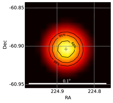
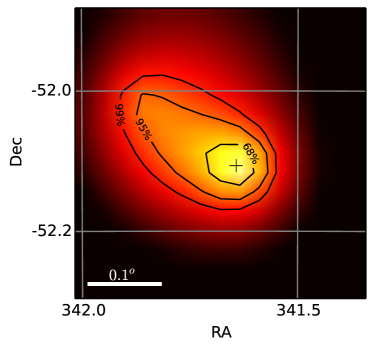
An important issue is how to treat apparently significant sources that do not have good localization fits, which we defined as LQ . An example is shown in Figure 5 (right). We flagged such sources (Flag 9 in Table 3) and for them estimated the position and uncertainty by performing a moment analysis of the LTS function instead of fitting a quadratic form. Some sources that did not have a well-defined peak in the likelihood were discarded by hand, on the consideration that they were most likely related to residual diffuse emission. Another possibility is that two nearby sources produce a dumbbell-like shape; for some of these cases we added a new source by hand. A final selection demanding that the semi-major radius () be less than resulted in 3976 candidate sources of which 142 were localized using the moment analysis.
As in 1FGL and 2FGL, we compared the localizations of the brightest sources with associations with their true positions in the sky. This indicated that the absolute precision is still the same, at the 95% confidence level. After the associations procedure (§ 5.2), we compared the distribution of distances to the high-confidence counterparts (in units of the estimated errors) with a Rayleigh distribution, and noted that it was slightly broader, by a factor 1.05 (smaller than the 1.1 factor used in 1FGL and 2FGL). Consequently, we multiplied all error estimates by 1.05 and added 0005 in quadrature to both 95% ellipse axes. The resulting comparison with the Rayleigh distribution is shown in Figure 3 of Ackermann et al. (2015, 3LAC) and indicates good agreement.
3.1.4 Detection of additional sources
We used the definition of likelihood itself to detect sources that needed to be added to the model of the sky. Using HEALPix with , we defined 3.2 M pixels in the sky, separated by , then evaluated the improvement in the likelihood from adding a new point source at the center of each, assuming a power-law spectrum with index 2.2. The value for each attempt, assigned to the pixel, defines a residual map of the sky. Next we performed a cluster analysis for all pixels with , determining the number of pixels, the maximum , and the -weighted centroid. All such clusters with at least two pixels were added to a list of seeds. Then each seed was reanalyzed, now allowing the spectral index to vary, with a full optimization in the respective RoI, and then localized. The last step was to add all such refit seeds, if the fits to the spectrum and the position were successful, and , as new sources, for a final optimization of the full sky.
3.2 Significance and Thresholding
The framework for this stage of the analysis is inherited from the 2FGL catalog. It splits the sky into RoIs, varying typically half a dozen sources near the center of the RoI at the same time. There were 840 RoIs for 3FGL, listed in the ROIs extension of the catalog (App. A). The global best fit is reached iteratively, injecting the spectra of sources in the outer parts of the RoI from the previous step. In that approach the diffuse emission model (§ 2.3) is taken from the global templates (including the spectrum, unlike what is done with in § 3.1) but it is modulated in each RoI by three parameters: normalization and small corrective slope of the Galactic component and normalization of the isotropic component. Appendix A shows how those parameters vary over the sky.
Among more than 4000 seeds coming from the localization stage, we keep only sources at , corresponding to a significance of just over evaluated from the distribution with 4 degrees of freedom (position and spectral parameters, Mattox et al., 1996). The model for the current RoI is readjusted after removing each seed below threshold, so that the final model fits the full data. The low-energy flux of the seeds below threshold (a fraction of which are real sources) can be absorbed by neighboring sources closer than the PSF radius. There is no pair of seeds closer than , so the neighbors are unaffected at high energy. The fixed sources outside the core of the RoI are not tested and therefore not removed during the last fit of an RoI. Since the threshold at the previous step was set to 16, seeds with still populate the outer parts of the RoI, preventing the background level to rise (bullet 5 below).
We introduced a number of improvements with respect to 2FGL (by decreasing order of importance):
-
1.
After 2FGL was completed we understood that it was important to account for the different instrumental backgrounds in and events (§ 2.3). Implicitly assuming that they were equal as in 2FGL resulted in lower (fewer sources) and tended to underestimate the low-energy flux. The impact is largest at high latitude. We used different isotropic spectral templates for and events, but a common renormalization parameter. We also used different and models of the Earth limb. The same distinction was introduced for computing the fluxes per energy band (§ 3.5) and per month (§ 3.6).
-
2.
Another effect discovered after 2FGL was a slight inconsistency (8% at 100 MeV) between the and effective areas. This affected mostly the Galactic plane, where the strong interstellar emission makes up 90% of the events. That effect created opposite low-energy residuals in and which did not compensate each other because of the differing PSF. It was corrected empirically in the P7REP_SOURCE_V15 version of the IRFs (Bregeon et al., 2013).
-
3.
We put in place an automatic iteration procedure at the next-to-last step of the process checking that the all-sky result is stable (2FGL used a fixed number of five iterations), similar to what was done for localization in 2FGL. Quantitatively, we iterated an RoI and its neighbors until did not change by more than 10. In practice this changes nothing at high latitude, but improves convergence in the Galactic plane. Fifteen iterations were required to reach full convergence. That iteration procedure was run twice, allowing sources to switch to a curved spectral shape (§ 3.3) after the first convergence.
-
4.
The software issue which prevented using unbinned likelihood in 2FGL was solved. We took advantage of that by using unbinned likelihood at high energy where keeping track of the exact direction of each event helps. At low energy we used binned likelihood in order to cap the memory and CPU resources. The dividing energy was set to 3 GeV, resulting in data cubes (below 3 GeV) and event lists (above 3 GeV) of approximately equal size. Both data sets were split between and . This was implemented in the framework of . In binned mode, the pixel size was set to and for and events, respectively (at 3 GeV the full width at half maximum of the PSF is and , respectively). The energy binning was set to 10 bins per decade as in 2FGL. In the exposure maps for unbinned mode, the pixel size was set to (even though the exposure varies very slowly, this is required to model precisely the edge of the field of view).
-
5.
We changed the criterion for including sources outside the RoI in the model. We replaced the flat distance threshold by a threshold on contributed counts (predicted from the model at the previous step). We kept all sources contributing more than 2% of the counts per square degree in the RoI. This is a good compromise between reliability and memory/CPU requirements, and accounts for bright sources even far outside the RoI (at 100 MeV the 95% containment radius for events is ). Compared to 2FGL, that new procedure affects mostly high latitudes (where the sources make up a larger fraction of the diffuse emission). Because it brings more low-energy events from outside in the model, it tends to reduce the fitted level of the low-energy diffuse emission, resulting in slightly brighter and softer source spectra.
-
6.
The fits are now performed up to 300 GeV, and the overal significances (Signif_Avg) as well as the spectral parameters refer to the full 100 MeV to 300 GeV band.
- 7.
-
8.
For homogeneity (so that the result does not depend on which spectral model we start from) the threshold was always applied to the power-law model, even if the best-fit model was curved. There are 21 sources in 2FGL with which would not have made it with this criterion (see § 3.3 for the definition of ).
3.3 Spectral Shapes
The spectral representation of sources was mostly the same as in 2FGL. We introduced an additional parameter modeling a super- or subexponentially cutoff power law, as in the pulsar catalog (Abdo et al., 2013). However this was applied only to the brightest pulsars (PSR J08354510 in Vela, J0633+1746, J17094429, J1836+5925, J0007+7303). The global fit with nearby sources was too unstable for the fainter ones, which were left with a simple exponentially cutoff power law. The subexponentially cutoff power law was also adopted for the brightest blazar 3C 454.3999That is only a mathematical model, it should not be interpreted in a physical sense since it is an average over many different states of that very variable object.. The fit was very significantly better than with either a log-normal or a broken power law shape. Even though bright sources are not a scientific objective of a catalog, avoiding low-energy spectral residuals (which translate into spatial residuals because of the broad PSF) is important for nearby sources.
Therefore the spectral representations which can be found in 3FGL are:
-
•
a log-normal representation (LogParabola in the tables) for all significantly curved spectra except pulsars and 3C 454.3:
(1) where is the natural logarithm. The reference energy is set to Pivot_Energy in the tables. The parameters , (spectral slope at ) and the curvature appear as Flux_Density, Spectral_Index and beta in the tables, respectively. No negative (spectrum curved upwards) was found. The maximum allowed was set to 1 as in 2FGL.
-
•
an exponentially cutoff power law for all significantly curved pulsars and a super- or subexponentially cutoff power law for the bright pulsars and 3C 454.3 (PLExpCutoff or PLSuperExpCutoff in the tables, depending on whether was fixed to 1 or left free):
(2) where the reference energy is set to Pivot_Energy in the tables and the parameters , (low-energy spectral slope), (cutoff energy) and (exponential index) appear as Flux_Density, Spectral_Index, Cutoff and Exp_Index in the tables, respectively. Note that this is not the way that spectral shape appears in the Science Tools (no term in the exponential), so the error on in the tables was obtained from the covariance matrix. The minimum was set to 0.5 (in 2FGL it was set to 0).
-
•
a simple power-law form for all sources not significantly curved.
As in 2FGL, a source is considered significantly curved if where (curved spectrum)(power-law)). The curved spectrum is PLExpCutoff (or PLSuperExpCutoff) for pulsars and 3C 454.3, LogParabola for all other sources. The curvature significance is reported as Signif_Curve (see § 3.5).
Another difference with 2FGL is that the complex spectrum of the Crab was represented as three components:
-
•
a PLExpCutoff shape for the pulsar, with free , and .
-
•
a soft power-law shape for the synchrotron emission of the nebula, with free and since the synchrotron emission is variable (Abdo et al., 2011c). The synchrotron component is called 3FGL J0534.5+2201s.
-
•
a hard power-law shape for the inverse Compton emission of the nebula, with parameters fixed to those found in Abdo et al. (2010e). That component does not vary, and leaving it free made the fit unstable. It is called 3FGL J0534.5+2201i.
In 2FGL, two sources (MSH 1552 and Vela X) spatially coincident with pulsars had trouble converging and their spectra were fixed to the result of the dedicated analysis (Abdo et al., 2010a, g). In 3FGL the spectra of five sources were fixed for the same reason: the same two, the Inverse Compton component of the Crab Nebula, the Cygnus X cocoon (Ackermann et al., 2011a) and the -Cygni supernova remnant. The spatial template of -Cygni was taken from Lande et al. (2012) as in 1FHL. We did not switch to the more complex spatial template used in Ackermann et al. (2011a) but the spectral template was obtained from a reanalysis of the Cygnus region including the Cygnus X cocoon (L. Tibaldo, private communication).
Overall in 3FGL six sources (the five brightest pulsars and 3C 454.3) were fit as PLSuperExpCutoff (with of Eq. 2 ), 110 pulsars were fit as PLExpCutoff, 395 sources were fit as LogParabola and the rest (including the five fixed sources) were represented as power laws.
3.4 Extended Sources
As for the 2FGL and 1FHL catalogs, we explicitly model as spatially extended those LAT sources that have been shown in dedicated analyses to be resolved by the LAT. Twelve extended sources were entered in the 2FGL catalog. That number grew to 22 in the 1FHL catalog. The spatial templates were based on dedicated analysis of each source region and have been normalized to contain the entire flux from the source ( of the flux for unlimited spatial distributions such as 2-D Gaussians). The spectral form chosen for each source is the best adapted among those used in the catalog analysis (see § 3.3). Three more extended sources have been reported since then and were included in the same way in the 3FGL analysis101010The templates and spectral models are available through the Fermi Science Support Center..
The catalog process does not involve looking for new extended sources or testing possible extension of sources detected as point-like. This was last done comprehensively by Lande et al. (2012) based on 1FGL. The extended sources published since then were the result of focussed studies so there most likely remain unreported faint extended sources in the Fermi-LAT data set. The process does not attempt to refit the spatial shape of known extended sources either.
The extended sources include twelve supernova remnants (SNRs), nine pulsar wind nebulae (PWNe) or candidates, the Cygnus X cocoon, the Large and Small Magellanic Clouds (LMC and SMC), and the lobes of the radio galaxy Centaurus A. Below we provide notes on new sources and changes since 2FGL:
- •
-
•
HESS J1303631 and HESS J1841055 are two H.E.S.S. sources (most likely PWNe) recently reported as faint hard LAT sources by Acero et al. (2013). We added them to the list, using the original H.E.S.S. template rather than the best spatial fit to the LAT data, in keeping with the spectral analysis in that paper.
-
•
We changed the spectral representation of the LMC and the Cygnus Loop from PLExpCutoff to LogParabola, which fits the data better. The curvature of the fainter SMC spectrum is not significant; therefore it was fit as a power law.
In general, we did not allow any point source inside the extended templates, even when the maps indicated that adding new seeds would improve the fit. Most likely (pending a dedicated reanalysis) those additional seeds were simply residuals due to the fact that the very simple geometrical representations that we adopted are not precise enough, rather than independent point sources. We preferred not splitting the source flux into pieces. The only exceptions are 3FGL J1823.21339 within HESS J1825137, 3FGL J2053.9+2922 inside the Cygnus Loop, 3FGL J0524.56937 inside the LMC, and sources inside the Cygnus X cocoon. The first one is as significant as the extended source and was a 2FGL source already. The next two are well localized over large extended sources and show a very hard spectrum, so they do not impact the spectral characteristics of the extended sources. The Cygnus X cocoon was fixed (§ 3.3) and allowing point sources on top of it was necessary to reach a reasonable representation of the region.
Table 1 lists the source name, spatial template description, spectral form and the reference for the dedicated analysis. These sources are tabulated with the point sources, with the only distinction being that no position uncertainties are reported and their names end in e (see § 4.1). Unidentified point sources inside extended ones are marked by “xxx field” in the ASSOC2 column of the catalog.
| 3FGL Name | Extended Source | Spatial Form | Extent (deg) | Spectral Form | Reference |
|---|---|---|---|---|---|
| J0059.07242e | SMC | 2D Gaussian | 0.9 | PowerLaw | Abdo et al. (2010b) |
| J0526.66825e | LMC | 2D GaussianaaCombination of two 2D Gaussian spatial templates. | 1.2, 0.2 | LogParabola | Abdo et al. (2010k) |
| J0540.3+2756e | S 147 | Map | PowerLaw | Katsuta et al. (2012) | |
| J0617.2+2234e | IC 443 | 2D Gaussian | 0.26 | LogParabola | Abdo et al. (2010j) |
| J0822.64250e | Puppis A | Disk | 0.37 | PowerLaw | Lande et al. (2012) |
| J0833.14511e | Vela X | Disk | 0.88 | PowerLaw | Abdo et al. (2010g) |
| J0852.74631e | Vela Junior | Disk | 1.12 | PowerLaw | Tanaka et al. (2011) |
| J1303.06312e | HESS J1303631 | 2D Gaussian | 0.16 | PowerLaw | Aharonian et al. (2005) |
| J1324.04330e | Centaurus A (lobes) | Map | PowerLaw | Abdo et al. (2010c) | |
| J1514.05915e | MSH 1552 | Disk | 0.25 | PowerLaw | Abdo et al. (2010a) |
| J1615.35146e | HESS J1614518 | Disk | 0.42 | PowerLaw | Lande et al. (2012) |
| J1616.25054e | HESS J1616508 | Disk | 0.32 | PowerLaw | Lande et al. (2012) |
| J1633.04746e | HESS J1632478 | Disk | 0.35 | PowerLaw | Lande et al. (2012) |
| J1713.53945e | RX J1713.73946 | Map | PowerLaw | Abdo et al. (2011d) | |
| J1801.32326e | W28 | Disk | 0.39 | LogParabola | Abdo et al. (2010f) |
| J1805.62136e | W30 | Disk | 0.37 | LogParabola | Ajello et al. (2012) |
| J1824.51351e | HESS J1825137 | 2D Gaussian | 0.56 | LogParabola | Grondin et al. (2011) |
| J1836.50655e | HESS J1837069 | Disk | 0.33 | PowerLaw | Lande et al. (2012) |
| J1840.90532e | HESS J1841055 | 2D GaussianbbThe shape is elliptical; each pair of parameters represents the semi-major and semi-minor axes. | (0.41, 0.25) | PowerLaw | Aharonian et al. (2008) |
| J1855.9+0121e | W44 | RingbbThe shape is elliptical; each pair of parameters represents the semi-major and semi-minor axes. | (0.22, 0.14), (0.30, 0.19) | LogParabola | Abdo et al. (2010i) |
| J1923.2+1408e | W51C | DiskbbThe shape is elliptical; each pair of parameters represents the semi-major and semi-minor axes. | (0.40, 0.25) | LogParabola | Abdo et al. (2009b) |
| J2021.0+4031e | -Cygni | Disk | 0.63 | PowerLaw | Lande et al. (2012) |
| J2028.6+4110e | Cygnus X cocoon | 2D Gaussian | 2.0 | PowerLaw | Ackermann et al. (2011a) |
| J2045.2+5026e | HB 21 | Disk | 1.19 | LogParabola | Pivato et al. (2013) |
| J2051.0+3040e | Cygnus Loop | Ring | 0.7, 1.6 | LogParabola | Katagiri et al. (2011) |
Note. — List of all sources that have been modeled as extended sources. The Extent column indicates the radius for Disk sources, the dispersion for Gaussian sources, and the inner and outer radii for Ring sources.
3.5 Flux Determination
|

|
The source photon fluxes are reported in the same five energy bands (100 to 300 MeV; 300 MeV to 1 GeV; 1 to 3 GeV; 3 to 10 GeV; 10 to 100 GeV) as in 2FGL. The fluxes were obtained by freezing the spectral index to that obtained in the fit over the full range and adjusting the normalization in each spectral band. For the curved spectra (§ 3.3) the spectral index in a band was set to the local spectral slope at the logarithmic mid-point of the band , restricted to be in the interval [0,5]. The photon flux between 1 and 100 GeV as well as the energy flux between 100 MeV and 100 GeV ( and in Table 5; the subscript indicates the energy range as 10i–10j MeV), are derived from the full-band analysis assuming the best spectral shape, and their uncertainties from the covariance matrix. Even though the full analysis is carried out up to 300 GeV in 3FGL, we have not changed the energy range over which we quote fluxes so that they can be easily compared with past fluxes. The photon flux above 100 GeV is negligible anyway and the energy flux above 100 GeV is not precisely measured (even for hard sources).
Improvements with respect to the 2FGL analysis are:
-
•
We used binned likelihood in the first three bands (up to 3 GeV) and unbinned likelihood in the last two bands, distinguishing and events. The pixel sizes in each band in binned mode were and , and , and where in each band, the first value is for , the second one for . This reduces error bars by 10–15% compared to mixing and events as in 2FGL.
-
•
Following what was done in the 1FHL catalog, the errors on the fluxes of moderately faint sources ( in the band) were computed as errors with MINOS in the Minuit111111http://lcgapp.cern.ch/project/cls/work-packages/mathlibs/minuit/home.html. package. This was done whenever the relative error on flux in the quadratic approximation (from the covariance matrix) was larger than 10%. Both errors (lower and upper) are reported in the FITS table (App. B). The lower error is reported with a minus sign (when the error comes from the quadratic approximation, the lower error is simply minus the upper error). The upper limits for very faint sources () were computed as in 2FGL, using the Bayesian method (Helene, 1983) at 95% of the posterior probability. The upper error is then reported as where is the best-fit flux, and the lower error is set to NULL.
-
•
The same iteration procedure described in § 3.2 was put in place for the fluxes per energy band using a more stringent criterion (). Convergence was fast at high energy (little cross-talk between sources). It was a little slower at low energy (6 iterations in the first band) but much faster than the full-band fit because no spectral adjustment was involved.
-
•
We report as nuFnuxxx_yyy the Spectral Energy Distribution (SED) in the band defined by xxx to yyy MeV, which can be directly overlaid on an SED plot. The SED was obtained by dividing the energy flux in the band by the band width in natural logarithm log(yyy/xxx). Since the fit is performed on the flux only (no spectral freedom in each band), the relative error on the SED is the same as that on the corresponding flux.
As in 2FGL we report in 3FGL a curvature significance Signif_Curve = (in units) after approximately accounting for systematic uncertainties on effective area via
| (3) |
where runs over all bands, is the flux predicted by the power-law model and is the flux predicted by the best-fit (curved) model in that band from the spectral fit to the full band. reflects the systematic uncertainty on effective area (§ 3.7). The values were set to 0.1, 0.05, 0.05, 0.05, 0.1 in our five bands (the fourth one went down from 0.08 in 2FGL, thanks to improved calibration). Eq. 3 is not exactly the same formula used for 2FGL. In 2FGL would have been replaced by . The disadvantage of the previous estimate was that it capped Signif_Curve to rather low values (below 15) resulting in a small dynamic range because the largest relative systematic errors are in the two extreme bands and in those bands the power-law fit can run way above the points (because the spectra are curved downwards). Using the curved fit (closer to the points) to estimate the systematic errors is a more reasonable procedure, and recovers a larger dynamic range (up to 85 in 3FGL).
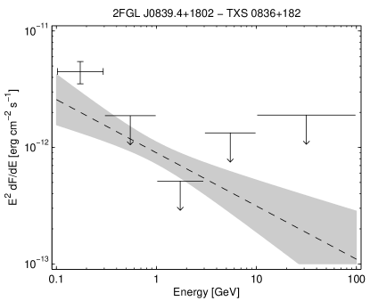
As in 2FGL we consider that only sources with Signif_Curve 4 are significantly curved (at the level). When is small (bright source) it can happen that (triggering a curved model following § 3.3) but Signif_Curve 4. The 43 such sources with LogParabola spectra (and 2 pulsars with PLExpCutoff spectra) but Signif_Curve 4 could be power laws within systematic errors. Nevertheless we do not go back to power-law spectra for those sources because they are better fit with curved models and power-law models would result in negative low-energy residuals which might affect nearby sources. One of them is illustrated in Figure 8. All are bright sources with modest curvature.
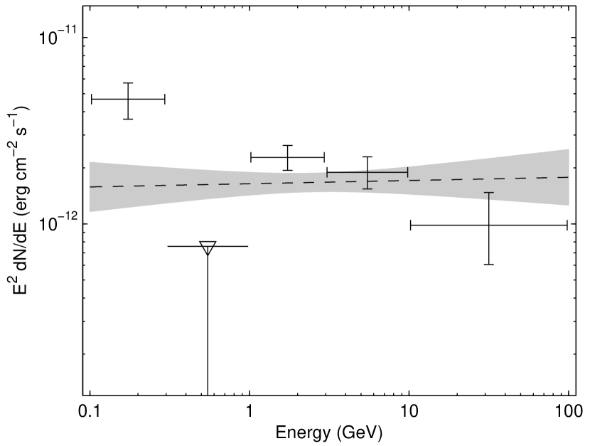
Spectral fit quality (for Flag 10 in Table 3) is computed as in Eq. 3 of Nolan et al. (2012, 2FGL) rather than as in § 3.1.1. Among the 42 sources flagged because of a too large spectral fit quality, most show deviations at low energy and are in confused regions or close to a brighter neighbor, as in Figure 9.
Spectral plots for all 3FGL sources overlaying the best model on the individual SED points are available from the FSSC.
3.6 Variability

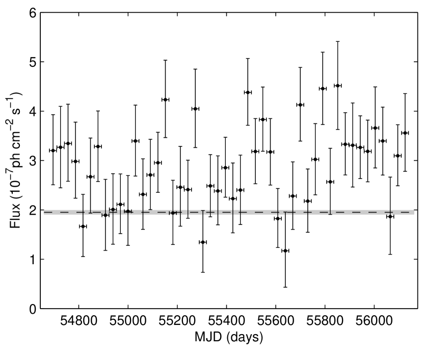
The light curves were computed over the same (1-month) intervals as in 1FGL and 2FGL (there are now 48 points). The first 23 intervals correspond exactly to 2FGL. The fluxes in each bin were obtained by freezing the spectral parameters to those obtained in the fit over the full range and adjusting the normalization. We used unbinned likelihood over the full energy range for the light curves. Over short intervals it does not incur a large CPU or memory penalty and it preserves the full information. We used a different isotropic and Earth limb model for and events, as in the main fit (§ 3.2). We also used a different Sun/Moon model for each month (the Sun is obviously at a different place in the sky each month). That improvement, together with our removing the solar flares, effectively mitigated the peaks that we noted in the 2FGL light curves due to the Sun passage near the source (Flag 11 in Table 3). We have not noted any obvious Sun-related peak in the 3FGL light curves (Figure 10).
As in the band fluxes calculation (§ 3.5) the errors on the monthly fluxes of moderately faint sources () were computed as lower and upper errors with MINOS in Minuit. Both errors (lower and upper) are reported in the FITS table (Table 16) so the Unc_Flux_History column is a array. This allowed providing more information in the light curve plots121212These plots are available from the FSSC. by keeping points with error bars whenever (the lower error does not reach 0). When the 95% upper limit is converted into an upper error in the same way as in 2FGL and the band fluxes calculation.
We noted an inconsistency between the light curve and the flux from the main fit (over the full interval) in several extended sources, whereby the average of the light curve appears distinctly above the flux from the main fit. It is particularly obvious in Cen A lobes, HESS J1616508 (Figure 11), S 147, W28, and W30. We traced the problem to the fact that we used unbinned likelihood over the whole energy range for the light curves, but binned likelihood for the main fit below 3 GeV. We have not found any evidence that this affects the point sources. Since we do not expect variability in extended sources, we left this inconsistency in the catalog as a known feature.
The variability indicator Variability_Index is the same as in 2FGL, with the same relative systematic error of 2%. Variability is considered probable when Variability_Index exceeds the threshold of 72.44 corresponding to 99% confidence in a distribution with 47 degrees of freedom.
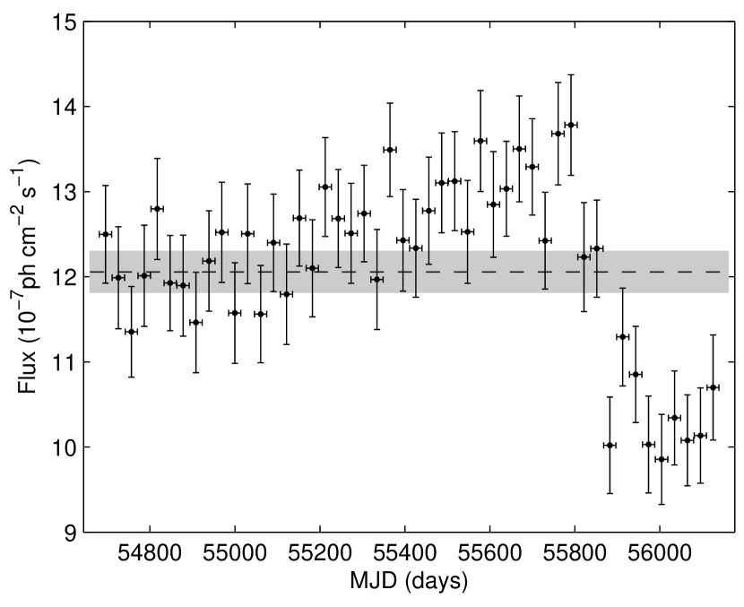
The Crab nebula and pulsar are a particularly difficult case. The nebula is very variable (Tavani et al., 2011; Abdo et al., 2011c) while the pulsar has no detected variability. So we would have liked the synchrotron component to absorb the full variability in 3FGL. It does not turn out this way, however, because the spectrum of the nebula becomes much harder during flares. This is not accounted for in the variability analysis (the spectral slopes are fixed to that in the full interval). As a result, the pulsar component also increases during the nebular flares and the pulsar becomes formally variable. We stress here that it is only a feature of our automatic analysis and is in no way a real detection of variability in the Crab pulsar. Besides the Crab, we detect the (real) variability of PSR J2021+4026 (Figure 12, Allafort et al., 2013). The only other formally variable pulsar is PSR J17323131 just above threshold. Since this is one in 137 pulsars, it is compatible with a chance occurrence at the 99% confidence level.
3.7 Limitations and Systematic Uncertainties
3.7.1 Source confusion

As for the 1FGL and 2FGL catalogs we investigated source confusion by comparing the actual distribution of angular separations between 3FGL sources with what would be expected for a population of sources that could be detected independently regardless how small their angular separations. The formalism is defined in Abdo et al. (2010d, 1FGL). We considered the region of the sky above , within which the average angular separation of 3FGL sources is . The distribution of nearest-neighbor distances is shown in Figure 13 along with the distribution expected if the source detection efficiency did not decrease for closely-spaced sources. The observed density of nearest-neighbor starts to fall below the expected curve at about angular separation. The implied number of missing closely-spaced sources is 140, or about 6% of the estimated true source count in the region. For the 2FGL catalog the fraction was only 3.3%. This indicates that even though the PSF improved after the Pass 7 reprocessing, the larger number of detected sources (2193 vs. 1319) is now pushing the LAT catalog into the confusion limit even outside the Galactic plane. Because the confusion process goes as the square of the source density, the expected number of sources above the detection threshold within of another one (most of which are not resolved) has increased by a factor of 3 between 2FGL and 3FGL.
The consequence of source confusion is not only losing a fraction of sources. It can also lead to “composite” -ray sources merging the characteristics of two very nearby astronomical objects. An example is the unassociated 3FGL J0536.43347, located between two bright blazars. Its spectrum is relatively soft, similar to that expected from the FSRQ BZQ J05363401, 14′ away. Its location, however, is closer (4′) to the BL Lac BZB J05363343 because that one dominates at high energy where the PSF is best. That issue is discussed in more detail in the 3LAC paper.
3.7.2 Instrument response functions
The systematic uncertainties on effective area have improved since 2FGL, going from P7SOURCE_V6 to P7REP_SOURCE_V15. They are now estimated to be 5% between 316 MeV and 10 GeV, increasing to 10% at 100 MeV and 15% at 1 TeV (see the caveats page at the FSSC), following the methods described by Ackermann et al. (2012a). As in previous LAT catalogs, we have not included those uncertainties in any of the error columns, because they apply uniformly to all sources. They must be kept in mind when working with absolute numbers, but comparisons between sources can be carried out at better precision. The systematic uncertainties on effective area have been included in the curvature significance (§ 3.5) and a systematic uncertainty of 2% on the stability of monthly flux measurements (measured directly on the bright pulsars) has been included in the variability index (§ 3.6).
3.7.3 Diffuse emission model
| Selection | Quantity | Diffuse model (§ 3.7.3) | Analysis method (§ 3.7.4) | ||
|---|---|---|---|---|---|
| Bias | Scatter | Bias | Scatter | ||
| Galactic | Eflux (174) | (+21%) | (42%) | (7%) | (27%) |
| Ridge | Index (88) | (+0.14) | (0.37) | (0.01) | (0.21) |
| Galactic | Eflux (662) | (+7%) | (32%) | (12%) | (23%) |
| Plane | Index (470) | (+0.04) | (0.21) | (0.06) | (0.15) |
| High | Eflux (2193) | (+1%) | (15%) | (7%) | (13%) |
| Latitude | Index (1960) | (+0.03) | (0.10) | (0.05) | (0.10) |
The model of diffuse emission is the main source of uncertainties for faint sources. Contrary to the effective area, it does not affect all sources equally: its effects are smaller outside the Galactic plane where the diffuse emission is fainter and varying on larger angular scales. It is also less of a concern in the high-energy bands ( 3 GeV) where the core of the PSF is narrow enough that the sources dominate the background under the PSF. But it is a serious concern inside the Galactic plane in the low-energy bands ( 1 GeV) and particularly inside the Galactic ridge () where the diffuse emission is strongest and very structured, following the molecular cloud distribution. It is not easy to assess precisely how large the uncertainties are, because they relate to uncertainties in the distributions of interstellar gas, the interstellar radiation field, and cosmic rays, which depend in detail on position on the sky.
For an assessment we have tried re-extracting the source spectra using one of the eight alternative interstellar emission models described in de Palma et al. (2013), namely the one obtained with optically thin H i, an SNR cosmic-ray source distribution and a 4 kpc halo, adapted to the P7REP IRFs. For computational reasons we have not used all eight alternative models, but that one should be representative. In each RoI we left free the normalization of each component of the model contributing (with its normalization set to 1) more than 3% of the total counts in the RoI. The isotropic normalization was also left free, but the inverse Compton, Loop I and Fermi bubbles components were fixed (too large scale to be fitted inside a single RoI). That approach (independent components) differs enough from the standard diffuse model that it can provide a stronger test than comparing with the previous generation diffuse model, as we did for 2FGL. Nevertheless both models still rely on nearly the same set of H i and CO maps of the gas in the interstellar medium, so they are not as independent as we would like.
The results show that the systematic uncertainty more or less follows the statistical one, i.e., it is larger for fainter sources in relative terms. We list the induced biases and scatters of flux and spectral index in Table 2. We have not increased the flux and index errors in the catalog itself accordingly because this alternative model does not fit the data as well as the newer one. The fit quality is nearly everywhere worse, except near the Carina region where we know the standard model does not fit the data very well (App. A). From that point of view we may expect these estimates of the systematic uncertainties to be upper limits. So we regard the values as qualitative estimates. In the Galactic plane (and even worse in the Galactic ridge) the systematic uncertainties coming from the diffuse model are larger than the statistical ones. In the Galactic ridge, even the bias is larger than the statistical uncertainty. The effect is larger than what we estimated for 2FGL (even though the diffuse model has improved), partly because the exposure is twice as deep and partly because the new alternative model is further from the standard one. Outside the Galactic plane the systematic uncertainty due to the diffuse model remains less than the statistical one, and the bias is negligible.
The same comparison also allows flagging outliers as suspect (§ 3.9). 119 sources received Flag 1 (Table 3) because they ended up with with the alternative model, and 118 received Flag 3, indicating that their photon or energy fluxes changed by more than . That uncertainty also appears in Flag 4 whereby we flag all sources with source-to-background ratio less than 10% in all bands in which they are statistically significant.
3.7.4 Analysis method
The check presented in this section is new to 3FGL. As explained in § 3.1 the -based method used to detect and localize sources also provides an estimate of the source spectra and significance. Therefore we use it to estimate systematic errors due to the analysis itself. Many aspects differ between the two methods: the code, the RoIs, the Earth limb representation. The alternative method does not remove faint sources (with ) from the model. The diffuse model is the same spatially but it was rescaled spectrally in each energy bin. The -based method also rescales in order to play down the energy bins in which the source-to-background ratio is low.
The procedure to compare the results is the same as in § 3.7.3. We list the induced biases and scatters of flux and spectral index in Table 2. In general, the effect of changing the analysis procedure is less than changing the diffuse model. Outside the Galactic ridge (and even outside the Galactic plane), we observe a negative bias on flux and index (i.e. fainter harder sources with the pipeline) close to half the statistical error. That effect is probably the result of removing the sources below threshold in the standard method. This favors absorbing the flux of faint neighbors at low energy (where the PSF is broad), resulting in somewhat brighter and softer sources.
A total of 118 sources received Flag 1 ( with ), and 101 received Flag 3 (flux changed by more than ). Only 25 (Flag 1) and 19 (Flag 3) sources are flagged from both the diffuse model and the analysis method comparisons. In other words, the 3FGL catalog is more or less half way between the result from and the result with the alternative diffuse model. Comparing the lists from and the alternative diffuse model would result in 202 sources with Flag 1 and 209 with Flag 3.
3.8 Sources Toward Local Interstellar Clouds and the Galactic Ridge
As we did for the 2FGL catalog, we carefully evaluated which sources are potentially artifacts due to systematic uncertainties in modeling the Galactic diffuse emission. The procedure, described in more detail in the 2FGL paper, flags unassociated sources with moderate and spectral index , corresponding to features in individual gas components. For 3FGL we did not consider sources that have very curved spectra to be artifacts. Very soft sources with power-law spectra are instead more likely to be problematic. Sources considered to be potential artifacts are assigned an analysis flag in the catalog (§ 3.9). We also append c to the source names.
Relative to the 2FGL catalog, far fewer c sources are flagged here (78 here vs. 162 for 2FGL) despite the much greater number of sources overall in the 3FGL catalog. Away from the Galactic plane, the reduction of c sources is primarily due to improvement of the representation of the dark gas component of the Galactic diffuse emission model in the vicinity of massive star-forming regions (§ 2.3). At low latitudes, the reduction primarily is due to relaxing the criterion on unassociated sources with very curved spectra.
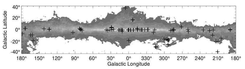
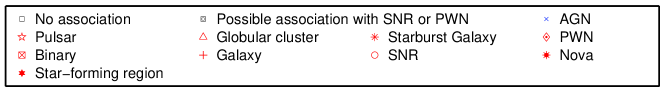
Figure 14 shows the locations of the c sources for 3FGL. The majority are close to the Galactic plane, where the diffuse -ray emission is brightest and very structured. Clusters are apparent in regions where spiral arms of the Milky Way are viewed essentially tangentially, in particular the Cygnus () and Carina () regions where the systematic uncertainties of the Galactic diffuse emission model are especially large. None of the c sources is identified (§ 5.1) and 63 (80%) have no firm association with a counterpart at other wavelengths, a much larger fraction than the overall average (30%) for 3FGL (Table 6).
3.9 Analysis Flags
| FlagaaIn the FITS version the values are encoded as individual bits in a single column, with Flag having value . For information about the FITS version of the table see Table 16 in App.B. | Meaning |
|---|---|
| 1 | Source with which went to when changing the diffuse model |
| (§ 3.7.3) or the analysis method (§ 3.7.4). Sources with are not flagged | |
| with this bit because normal statistical fluctuations can push them to . | |
| 2 | Not used. |
| 3 | Flux ( 1 GeV) or energy flux ( 100 MeV) changed by more than when |
| changing the diffuse model or the analysis method. Requires also that the flux | |
| change by more than 35% (to not flag strong sources). | |
| 4 | Source-to-background ratio less than 10% in highest band in which . |
| Background is integrated over or 1 square degree, whichever is smaller. | |
| 5 | Closer than from a brighter neighbor. is defined in the highest band in |
| which source , or the band with highest if all are . is set | |
| to (FWHM) below 300 MeV, between 300 MeV and 1 GeV, | |
| between 1 GeV and 3 GeV, between 3 and 10 GeV and above | |
| 10 GeV (). | |
| 6 | On top of an interstellar gas clump or small-scale defect in the model of |
| diffuse emission; equivalent to the c designator in the source name (§ 3.8). | |
| 7 | Unstable position determination; result from gtfindsrc outside the 95% ellipse |
| from pointlike. | |
| 8 | Not used. |
| 9 | Localization Quality 8 in pointlike (§ 3.1) or long axis of 95% ellipse . |
| 10 | Spectral Fit Quality (Eq. 3 of Nolan et al., 2012, 2FGL). |
| 11 | Possibly due to the Sun (§ 3.6). |
| 12 | Highly curved spectrum; LogParabola fixed to 1 or PLExpCutoff |
| Spectral_Index fixed to 0.5 (see § 3.3). |
As in 2FGL we identified a number of conditions that should be considered cautionary regarding the reality of a source or the magnitude of the systematic uncertainties of its measured properties. They are described in Table 3.
Each flag has the same definition as for the 2FGL catalog, except for Flag 7, which was unused in that catalog.
Flags 1 to 12 have similar intent as in 2FGL, but differ in detail:
- •
-
•
Flag 2 is not used. We didn’t go so far as to rerun the full detection and localization procedure (§ 3.1) with the alternative diffuse model. Assessing the changes in source characteristics is normally enough.
-
•
For Flag 4, we lowered the threshold for flagging the source-to-background ratio to 10%, recognizing that the uncertainties in the interstellar emission model are now reduced (App. A).
-
•
We reinstated Flag 7 (comparison between and localizations) which was not used in 2FGL because of an inconsistency in the unbinned likelihood results. It indicates sources for which the source locations derived from (§ 3.1.3) and are inconsistent at the 95% confidence level. was applied only above 3 GeV due to computing time constraints. This is appropriate for most sources (because the PSF is much better at high energy) but does not allow testing the localization of soft sources.
-
•
Flag 8 has been merged into Flag 9. Both tested localization reliability.
-
•
Flag 11 is deprecated because we put in place an explicit time-dependent model for the Sun and Moon emission (§ 2.3).
4 The 3FGL Catalog
We present a basic description of the 3FGL catalog in § 4.1, including a listing of the main table contents and some of the primary properties of the sources in the catalog. We present a detailed comparison of the 3FGL catalog with the 2FGL catalog in § 4.2.
4.1 Catalog Description
Table 4 is the catalog, with information for each of the 3033 sources131313Table 4 has 3034 entries because the PWN component of the Crab nebula is represented by two cospatial sources (§ 3.3).; see Table 5 for descriptions of the columns. The source designation is 3FGL JHHMM.m+DDMM where the 3 indicates that this is the third LAT catalog, FGL represents Fermi Gamma-ray LAT. Sources close to the Galactic ridge and some nearby interstellar cloud complexes are assigned names of the form 3FGL JHHMM.m+DDMMc, where the c indicates that caution should be used in interpreting or analyzing these sources. Errors in the model of interstellar diffuse emission, or an unusually high density of sources, are likely to affect the measured properties or even existence of these 78 sources (see § 3.8). In addition a set of analysis flags has been defined to indicate sources with unusual or potentially problematic characteristics (see § 3.9). The c designator is encoded as one of these flags. An additional 572 sources have one or more of the other analysis flags set. The 25 sources that were modeled as extended for 3FGL (§ 3.4) are singled out by an e appended to their names.
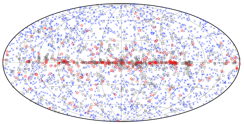
The designations of the classes that we use to categorize the 3FGL sources are listed in Table 6 along with the numbers of sources assigned to each class. Figure 15 illustrates where the source classes are in the sky. We distinguish between associated and identified sources, with associations depending primarily on close positional correspondence (see § 5.2) and identifications requiring measurement of correlated variability at other wavelengths or characterization of the 3FGL source by its angular extent (see § 5.1). In the cases of multiple associations with a 3FGL source, we adopt the single association that is statistically most likely to be true if it is above the confidence threshold (see § 5.2). Sources associated with SNRs are often also associated with PWNe and pulsars, and the SNRs themselves are often not point-like. We do not attempt to distinguish among the possible classifications and instead list in Table 7 plausible associations of each class for unidentified 3FGL sources found to be positionally associated with SNRs141414Four sources positionally associated with SNRs were also found to be associated with blazars. We cannot quantitatively compare association probabilities between the blazar and the (spatially extended) SNR classes. In the 3FGL catalog, we list only the blazar associations for them. The sources and SNR associations are 3FGL J0217.3+6209 (G137.2+01.3), 3FGL J0223.5+6313 (G132.7+01.3), 3FGL J0526.0+4253 (G166.0+04.3), and 3FGL J0215.6+3709 (G074.9+01.2).. The Crab pulsar and PWN are represented by a total of three entries, two of which (designated i and s) represent spectral components of the PWN (see § 5.1). We consider these three entries to represent two sources.
The photon flux for 1–100 GeV () and the energy flux for 100 MeV to 100 GeV in Table 4 are evaluated from the fit to the full band (see § 3.5). We do not present the integrated photon flux for 100 MeV to 100 GeV (see § 3.5). Table 8 presents the fluxes in individual bands as defined in § 3.5.
| Name 3FGL | R.A. | Decl. | Mod | Var | Flags | -ray Assoc. | TeV | ClassaaSee Table 6 for class designators. | ID or Assoc. | ||||||||||||
|---|---|---|---|---|---|---|---|---|---|---|---|---|---|---|---|---|---|---|---|---|---|
| J0000.1+6545 | 0.038 | 65.752 | 117.694 | 3.403 | 0.102 | 0.078 | 41 | 6.8 | 1.0 | 0.2 | 13.6 | 2.1 | 2.41 | 0.08 | PL | 3 | 2FGL J2359.6+6543c | ||||
| J0000.23738 | 0.061 | 37.648 | 345.411 | 74.947 | 0.073 | 0.068 | 89 | 5.1 | 0.2 | 0.1 | 2.4 | 0.7 | 1.87 | 0.18 | PL | ||||||
| J0001.0+6314 | 0.254 | 63.244 | 117.293 | 0.926 | 0.248 | 0.160 | 65 | 6.2 | 0.6 | 0.1 | 13.0 | 1.9 | 2.73 | 0.11 | PL | 3,4,5 | 2FGL J2358.9+6325 | spp | |||
| J0001.20748 | 0.321 | 7.816 | 89.022 | 67.324 | 0.082 | 0.070 | 19 | 11.3 | 0.7 | 0.1 | 7.8 | 0.9 | 2.15 | 0.09 | PL | 2FGL J0000.90748 | bll | PMN J00010746 | |||
| 1FGL J0000.90745 | |||||||||||||||||||||
| J0001.4+2120 | 0.361 | 21.338 | 107.665 | 40.047 | 0.211 | 0.188 | 33 | 11.4 | 0.3 | 0.1 | 8.1 | 0.8 | 2.78 | LP | T | 3EG J2359+2041 | fsrq | TXS 2358+209 | |||
| J0001.6+3535 | 0.404 | 35.590 | 111.661 | 26.188 | 0.213 | 0.167 | 8 | 4.2 | 0.3 | 0.1 | 3.4 | 0.8 | 2.35 | 0.19 | PL | 4 | |||||
| J0002.06722 | 0.524 | 67.370 | 310.139 | 49.062 | 0.102 | 0.086 | 69 | 5.9 | 0.3 | 0.1 | 3.3 | 0.8 | 1.95 | 0.16 | PL | ||||||
| J0002.24152 | 0.562 | 41.883 | 334.070 | 72.143 | 0.217 | 0.140 | 68 | 5.2 | 0.3 | 0.1 | 3.0 | 0.7 | 2.09 | 0.19 | PL | 2FGL J0001.74159 | bcu | 1RXS J000135.5415519 | |||
| 1FGL J0001.94158 | |||||||||||||||||||||
| J0002.6+6218 | 0.674 | 62.301 | 117.302 | 0.037 | 0.061 | 0.054 | 55 | 18.0 | 2.8 | 0.2 | 18.4 | 1.7 | 2.35 | LP | 2FGL J0002.7+6220 | ||||||
| J0003.25246 | 0.815 | 52.777 | 318.976 | 62.825 | 0.070 | 0.061 | 44 | 5.7 | 0.3 | 0.1 | 3.0 | 0.8 | 1.90 | 0.17 | PL | bcu | RBS 0006 | ||||
| J0003.4+3100 | 0.858 | 31.008 | 110.964 | 30.745 | 0.181 | 0.163 | 13 | 6.3 | 0.3 | 0.1 | 4.9 | 0.8 | 2.55 | 0.13 | PL | ||||||
| J0003.5+5721 | 0.890 | 57.360 | 116.486 | 4.912 | 0.089 | 0.072 | 1 | 5.4 | 0.5 | 0.1 | 5.4 | 1.1 | 2.18 | 0.13 | PL |
Note. — This table is published in its entirety in the electronic edition of the Astrophysical Journal Supplements. A portion is shown here for guidance regarding its form and content.
| Column | Description |
|---|---|
| Name | 3FGL JHHMM.m+DDMM[c/e/i/s], constructed according to IAU Specifications for Nomenclature; m is decimal |
| minutes of R.A.; in the name, R.A. and Decl. are truncated at 0.1 decimal minutes and 1′, respectively; | |
| c indicates that based on the region of the sky the source is considered to be potentially confused | |
| with Galactic diffuse emission; e indicates a source that was modeled as spatially extended (see § 3.4); | |
| the two spectral components of the Crab PWN are designated i and s | |
| R.A. | Right Ascension, J2000, deg, 3 decimal places |
| Decl. | Declination, J2000, deg, 3 decimal places |
| Galactic Longitude, deg, 3 decimal places | |
| Galactic Latitude, deg, 3 decimal places | |
| Semimajor radius of 95% confidence region, deg, 3 decimal places | |
| Semiminor radius of 95% confidence region, deg, 3 decimal places | |
| Position angle of 95% confidence region, deg. East of North, 0 decimal places | |
| Significance derived from likelihood Test Statistic for 100 MeV–300 GeV analysis, 1 decimal place | |
| Photon flux for 1 GeV–100 GeV, 10-9 ph cm-2 s-1, summed over 3 bands, 1 decimal place | |
| uncertainty on , same units and precision | |
| Energy flux for 100 MeV–100 GeV, 10-12 erg cm-2 s-1, from power-law fit, 1 decimal place | |
| uncertainty on , same units and precision | |
| Photon number power-law index, 100 MeV–100 GeV, 2 decimal places | |
| uncertainty of photon number power-law index, 100 MeV–100 GeV, 2 decimal places | |
| Mod. | PL indicates power-law fit to the energy spectrum; LP indicates log-parabola fit to the energy spectrum; |
| EC indicates power-law with exponential cutoff fit to the energy spectrum | |
| Var. | T indicates 1% chance of being a steady source; see note in text |
| Flags | See Table 3 for definitions of the flag numbers |
| -ray Assoc. | Positional associations with 0FGL, 1FGL, 2FGL, 3EG, EGR, or 1AGL sources |
| TeV | Positional association with a TeVCat source, P for unresolved angular size, E for extended |
| Class | Like ‘ID’ in 3EG catalog, but with more detail (see Table 6). Capital letters indicate firm identifications; |
| lower-case letters indicate associations | |
| ID or Assoc. | Designator of identified or associated source |
| Description | Identified | Associated | ||
|---|---|---|---|---|
| Designator | Number | Designator | Number | |
| Pulsar, identified by pulsations | PSR | 143 | ||
| Pulsar, no pulsations seen in LAT yet | psr | 24 | ||
| Pulsar wind nebula | PWN | 9 | pwn | 2 |
| Supernova remnant | SNR | 12 | snr | 11 |
| Supernova remnant / Pulsar wind nebula | spp | 49 | ||
| Globular cluster | GLC | 0 | glc | 15 |
| High-mass binary | HMB | 3 | hmb | 0 |
| Binary | BIN | 1 | bin | 0 |
| Nova | NOV | 1 | nov | 0 |
| Star-forming region | SFR | 1 | sfr | 0 |
| Compact Steep Spectrum Quasar | CSS | 0 | css | 1 |
| BL Lac type of blazar | BLL | 18 | bll | 642 |
| FSRQ type of blazar | FSRQ | 38 | fsrq | 446 |
| Non-blazar active galaxy | AGN | 0 | agn | 3 |
| Radio galaxy | RDG | 3 | rdg | 12 |
| Seyfert galaxy | SEY | 0 | sey | 1 |
| Blazar candidate of uncertain type | BCU | 5 | bcu | 568 |
| Normal galaxy (or part) | GAL | 2 | gal | 1 |
| Starburst galaxy | SBG | 0 | sbg | 4 |
| Narrow line Seyfert 1 | NLSY1 | 2 | nlsy1 | 3 |
| Soft spectrum radio quasar | SSRQ | 0 | ssrq | 3 |
| Total | 238 | 1785 | ||
| Unassociated | 1010 | |||
Note. — The designation ‘spp’ indicates potential association with SNR or PWN (see Table 7). Designations shown in capital letters are firm identifications; lower case letters indicate associations. In the case of AGN, many of the associations have high confidence. Among the pulsars, those with names beginning with LAT were discovered with the LAT.
| Name 3FGL | SNR name | PWN name | TeV name | Common name |
|---|---|---|---|---|
| J0001.0+6314 | G116.5+01.1 | |||
| J0128.4+6257 | G127.1+00.5 | R5 | ||
| J0220.1+6202c | G132.7+01.3 | HB3 | ||
| J0224.0+6235 | G132.7+01.3 | HB3 | ||
| J0500.3+5237 | G156.2+05.7 | |||
| J0610.6+1728 | G192.801.1 | PKS 0607+17 | ||
| J0631.6+0644 | G205.5+00.5 | Monoceros Loop | ||
| J0640.9+0752 | G205.5+00.5 | Monoceros Loop | ||
| J0838.14615aaThese sources have been found to be significantly variable, i.e., Variability_Index (§ 3.6), which would be unexpected for physical associations with SNRs or PWNe. | G263.903.3 | Vela | ||
| J0839.14739 | G263.903.3 | Vela | ||
| J0843.14546 | G263.903.3 | Vela | ||
| J1101.96053 | G290.100.8 | MSH 1161A | ||
| J1111.96038 | G291.000.1 | G291.00.1 | MSH 1162 | |
| J1209.15224 | G296.5+10.0 | PKS 120951 | ||
| J1212.26251 | G298.500.3 | |||
| J1214.06236 | G298.600.0 | |||
| J1345.16224 | G308.800.1 | |||
| J1441.55955c | G316.300.0 | MSH 1457 | ||
| J1549.15347c | G327.4+00.4 | |||
| J1551.15610 | G326.301.8 | Kes 25 | ||
| J1552.95610 | G326.301.8 | Kes 25 | ||
| J1615.35146e | HESS J1614518 | |||
| J1628.94852 | G335.2+00.1 | |||
| J1636.24709c | G337.2+00.1 | HESS J1634472 | ||
| J1638.64654aaThese sources have been found to be significantly variable, i.e., Variability_Index (§ 3.6), which would be unexpected for physical associations with SNRs or PWNe. | G337.800.1 | Kes 41 | ||
| J1640.44634c | G338.300.0 | HESS J1640465 | ||
| J1641.14619c | G338.5+00.1 | HESS J1641463 | ||
| J1645.95420 | G332.505.6 | |||
| J1722.94529 | G343.006.0 | RCW 114 | ||
| J1725.12832 | G358.0+03.8 | |||
| J1728.04606 | G343.006.0 | RCW 114 | ||
| J1729.52824 | G358.0+03.8 | |||
| J1737.33214c | G356.300.3 | |||
| J1745.13011 | G359.100.5 | HESS J1745303 | ||
| J1745.62859c | G000.0+00.0 | G359.950.04 | Galactic Centre | Sgr A East |
| J1810.11910 | G011.1+00.1 | HESS J1809193 | ||
| J1811.31927c | G011.200.3 | HESS J1809193 | ||
| J1817.21739 | G013.301.3 | |||
| J1818.71528aaThese sources have been found to be significantly variable, i.e., Variability_Index (§ 3.6), which would be unexpected for physical associations with SNRs or PWNe. | G015.4+00.1 | |||
| J1828.41121aaThese sources have been found to be significantly variable, i.e., Variability_Index (§ 3.6), which would be unexpected for physical associations with SNRs or PWNe. | G020.000.2 | |||
| J1829.71304 | G018.901.1 | |||
| J1833.90711aaThese sources have been found to be significantly variable, i.e., Variability_Index (§ 3.6), which would be unexpected for physical associations with SNRs or PWNe. | G024.7+00.6 | |||
| J1834.60659 | G024.7+00.6 | |||
| J1840.10412 | G027.8+00.6 | |||
| J1915.9+1112 | G045.700.4 | |||
| J1951.6+2926 | G065.7+01.2 | |||
| J2014.4+3606 | G073.9+00.9 | |||
| J2022.2+3840 | G076.9+01.0 | |||
| J2225.8+6045 | G106.3+02.7 | G106.3+2.7 |
Note. — These sources are classified as spp in Table 4. They may be pulsars rather than the SNR or PWN named. Four additional 3FGL sources are associated with both an SNR and a blazar. For these the catalog lists the blazar associations; see text.
| 0.1–0.3 GeV | 0.3–1 GeV | 1–3 GeV | 3–10 GeV | 10–100 GeV | ||||||
|---|---|---|---|---|---|---|---|---|---|---|
| Name 3FGL | aaIn units of photons cm-2 s-1 | aaIn units of photons cm-2 s-1 | bbIn units of photons cm-2 s-1 | ccIn units of photons cm-2 s-1 | ccIn units of photons cm-2 s-1 | |||||
| J0000.1+6545 | 2.2 | 5.3 | 6.0 | 1.5 | 2.4 | |||||
| J0000.23738 | 0.0 | 0.6 | 2.9 | 4.2 | 3.5 | |||||
| J0001.0+6314 | 4.0 | 4.3 | 1.7 | 3.3 | 0.4 | |||||
| J0001.20748 | 1.6 | 5.3 | 7.0 | 8.0 | 1.6 | |||||
| J0001.4+2120 | 6.8 | 7.6 | 4.5 | 0.0 | 0.0 | |||||
| J0001.6+3535 | 3.6 | 0.9 | 2.5 | 2.0 | 2.3 | |||||
| J0002.06722 | 0.2 | 2.0 | 3.4 | 4.8 | 3.1 | |||||
| J0002.24152 | 2.5 | 2.1 | 1.5 | 4.7 | 2.6 | |||||
| J0002.6+6218 | 2.6 | 9.4 | 13.3 | 7.4 | 0.0 | |||||
| J0003.25246 | 1.8 | 0.0 | 3.1 | 3.7 | 4.5 | |||||
| J0003.4+3100 | 3.4 | 3.6 | 4.9 | 1.1 | 0.1 | |||||
| J0003.5+5721 | 0.0 | 3.5 | 4.0 | 3.3 | 3.0 | |||||
| J0003.81151 | 0.0 | 1.5 | 3.8 | 2.5 | 2.5 | |||||
| J0004.2+6757 | 0.5 | 4.4 | 3.4 | 3.2 | 1.4 | |||||
| J0004.2+0843 | 0.8 | 0.7 | 1.5 | 5.3 | 2.0 | |||||
Note. — This table is published in its entirety in the electronic edition of the Astrophysical Journal Supplements. A portion is shown here for guidance regarding its form and content.
4.2 Comparison with 0FGL, 1FGL, 2FGL and 1FHL
4.2.1 General comparison
We compare the 3FGL with previous catalogs released by the LAT collaboration. These are listed in Table 9.
| Category | 0FGLaa0FGL, the LAT Bright Source List, has a lower energy limit of 200 MeV and a significance threshold . | 1FGL | 2FGL | 1FHLbb1FHL is a catalog for the energy range 10 GeV. | 3FGL | |
|---|---|---|---|---|---|---|
| Total | 205 | 1451 | 1873 | 514 | 3033 | |
| High-Latitude sources | 132 | 1043 | 1319 | 399 | 2193 | |
| Low-Latitude sources | 73 | 408 | 554 | 115 | 841 | |
| ‘Lost’ sources(c)(c)footnotemark: in 3FGL | 12 | 310 | 300 | 17 | - |
Associations among 3FGL and 0FGL/1FGL/2FGL and 1FHL sources are based on the following relation:
| (4) |
where is the angular distance between the sources, is defined in terms of the semi-major axis of the % confidence error ellipse for the position of each source, e.g., the 95% confidence error for the automatic source association procedure (§ 5.2) and ‘a’ is alternatively 0FGL, 1FGL, 2FGL, and 1FHL. In total, 1720 3FGL sources were automatically associated with entries in either the 0FGL, 1FGL, 2FGL, or 1FHL catalogs. The statistics of the association results is reported in Table 13.
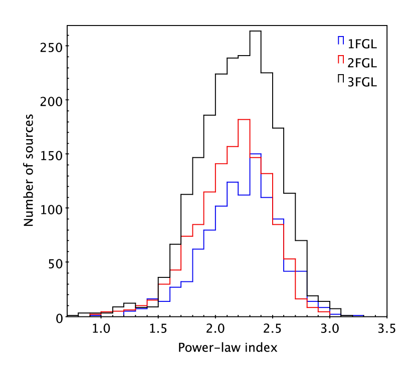
In the 3FGL analysis the spectral fits are made using power-law, power-law with an exponential cutoff, or log-parabola models (§ 3.3). For each 2FGL and 3FGL source we also evaluated the spectral index () of the best power-law fit and this enables a comparison of the spectral characteristics of the 1FGL, 2FGL, and 3FGL sources. Figure 16 shows the distributions of the power-law indices of the sources at high Galactic latitude and only those with a power-law spectral type in the 1FGL, 2FGL and 3FGL catalogs, to avoid possible confusion from more complex features. The three distributions are very similar, with an average , average , and average . However, the peaks of the three distributions are not exactly coincident; also, they have different skewnesses. The small differences in the power-law index distributions could be related to slightly different systematic uncertainties in the effective area between the instrument response functions P7REP_SOURCE_V15, P7SOURCE_V6 and P6_V3_DIFFUSE used respectively for 3FGL, 2FGL, and 1FGL.
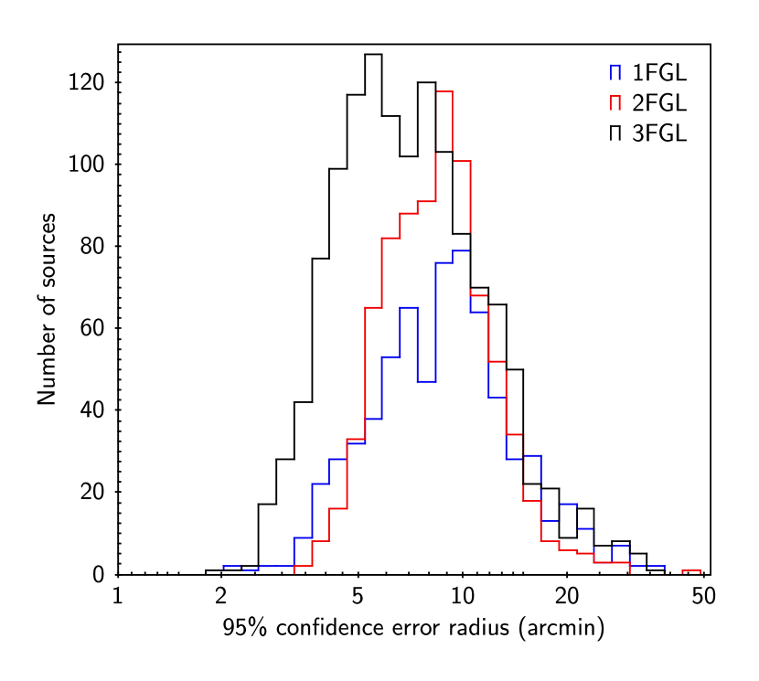
We have compared the distribution of the 95% confidence error radii of the 1FGL, 2FGL, and 3FGL sources at high Galactic latitude. The distribution of 95% confidence error radius for those sources with in any of the 1FGL, 2FGL, and 3FGL catalogs (Figure 17) shows the localization improvement for a given range of source detection significances. We evaluated the 95% confidence error radius as the geometric mean of the semi-major and semi-minor axes of the 95% confidence error ellipse.
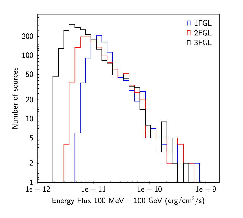
Figure 18 shows the energy flux distribution in 1FGL, 2FGL, and 3FGL. Comparing the current flux threshold with those published in previous LAT Catalog papers we see that in 3FGL the threshold is down to erg cm-2 s-1, from erg cm-2 s-1 in 2FGL and erg cm-2 s-1 in 1FGL. Above that flux the 2FGL and 3FGL distributions are entirely compatible.
However the 1FGL distribution shows a distinct bump between 1 and erg cm-2 s-1. That accumulation of fluxes was clearly incorrect. We attribute it primarily to overestimating significances and fluxes due to the unbinned likelihood bias in the 1FGL analysis, and also to the less accurate procedure then used to extract source flux (see discussion in the 2FGL paper).
4.2.2 Comparison of individual sources

Figure 19 shows the distribution of the differences and for the 621 high-latitude sources with power-law spectrum type in common among the three catalogs. The average of the 3FGL – 2FGL distribution is , with the 3FGL sources slightly softer than the 2FGL ones, while the average of the 3FGL – 1FGL distribution is , with the 3FGL sources slightly harder than the 1FGL ones.
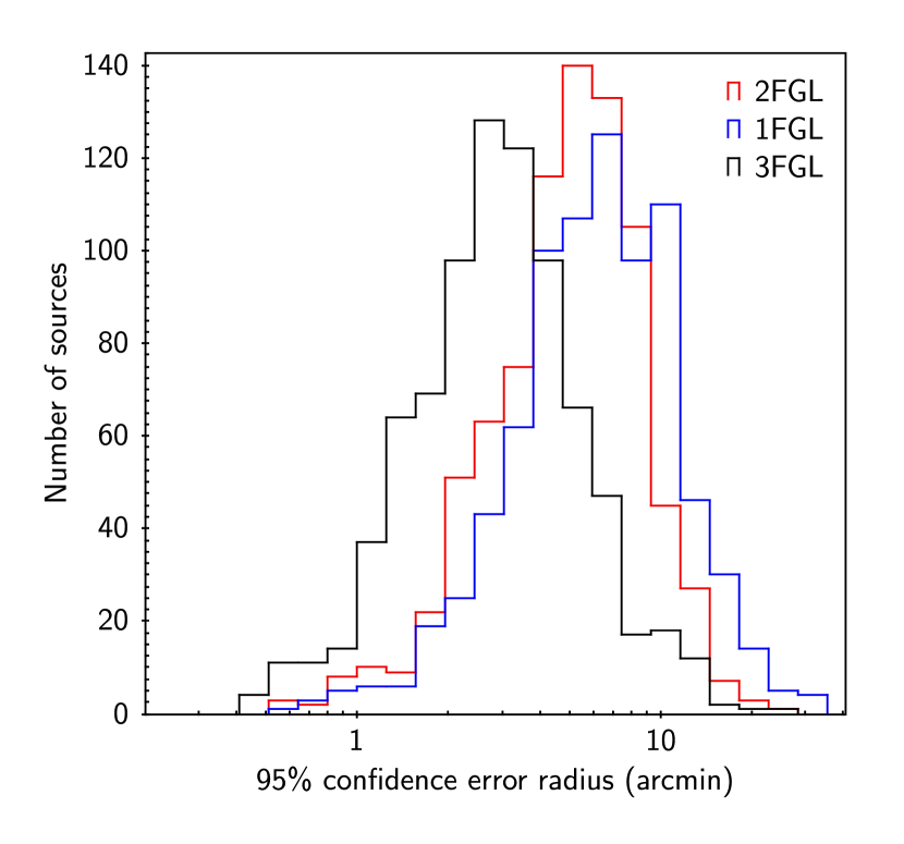
When comparing the distribution of 95% confidence error radius for the sources in common among all the LAT catalogs, we see that for 3FGL this parameter extends to lower values than for the earlier catalogs, showing that the localization has improved, thanks to improvements in the 3FGL analysis and increased statistics over the longer integration period for 3FGL (Figure 20).
4.2.3 Possible causes for losing sources
In the remainder of this section we describe a variety of reasons why the ‘lost’ 0FGL, 1FGL, 2FGL, and 1FHL sources might not appear in the 3FGL catalog. Table 10 shows the statistics of the ‘lost’ sources.
| 0FGL not in 3FGL | 1FGL not in 3FGL | 2FGL not in 3FGL | 1FHL not in 3FGL | ||
|---|---|---|---|---|---|
| All | 12 | 310 | 300 | 17 | |
| With flags | - | 131 | 211 | - | |
| Name-FGL c (a)(a)footnotemark: | - | 104 | 87 | - | |
| AGN | 1 | 22 | 27 | 1 | |
| PSR | 0 | 1 | 3 | 0 | |
| Unassociated | 11 | 264 | 234 | 16 | |
| Within 1° of a 3FGL e (b)(b)footnotemark: | 3 | 27 | 33 | 4 | |
| sources in other FGL catalogs | |||||
| 0FGL | - | 5 | 5 | 0 | |
| 1FGL | 4 | - | 56 | 1 | |
| 2FGL | 3 | 67 | - | 1 | |
| 1FHL | 0 | 2 | 8 | - | |
| Not in any other Fermi catalog | 7 | 237 | 237 | 15 |
We have also produced tables with all the ‘lost’ sources for each previous LAT catalog. The first rows of the ‘lost’ -ray source table for the 2FGL catalog are listed in Table 11, only reported for guidance.151515The full table of lost 2FGL sources and similar tables for lost 0FGL, lost 1FGL, and lost 1FHL sources are available only in the electronic version. In the last columns of Table 11 we assigned to each source one or more flags corresponding to possible causes for it to be lost and which we will discuss in the following paragraphs. In many cases, no one reason can be singled out.
Lost sources from previous LAT catalogs are in general equally distributed over all latitudes, with a slight excess at low latitudes for 2FGL ‘lost’ sources. In fact about 10% of the 2FGL ‘lost’ sources are at low Galactic latitude compared to a 6% of high-latitude ‘lost’ 2FGL sources. We remind the reader that at low latitudes the Galactic diffuse emission is most intense and improvements in the model for the diffuse emission would be expected to have the most influence (§ 2.3). The sources in common among 3FGL and the previous LAT catalogs are primarily outside the Galactic plane, as are the sources newly detected in 3FGL. Most of the ‘lost’ sources were also listed as unassociated in the previous FGL catalogs. Among the former associated ‘lost’ sources, most of them were associated with AGN and a few with pulsars. For sources of the AGN type their absence from the 3FGL catalog can be due to their intrinsic variability. A faint source which flared during the first year, allowing it to be detected in 0FGL, can be diluted and become undetectable in a longer time interval.
Most of the ‘lost’ sources have analysis flags or the c designator in 1FGL and 2FGL names, indicating that these sources were already flagged as influenced by the diffuse emission and recognized as potentially problematic or possibly spurious.
Some other 1FGL, 2FGL, and 1FHL sources do not have counterparts in the 3FGL catalog because they have been resolved into two or more 3FGL sources or candidate source seeds. We flag them with ‘S’ (split) in the ‘Flag’ column of Table 11. In some cases only one of the seeds reached and so was included in the 3FGL list.
Several other possible causes of ‘lost’ sources are evident: (1) the 3FGL -ray centroid has shifted with respect to the previous FGL catalogs, preventing the matching; (2) statistical threshold effects, i.e. their has dropped below 25. Additional considerations include variability and (generally small) effects from the different event selections used for the analyses (P7REP_SOURCE_V15 for 3FGL, P7CLEAN_V6 for 1FHL, P7SOURCE_V6 for 2FGL and P6_V3_DIFFUSE for 0FGL); different Galactic diffuse emission models; different analysis procedures (unbinned likelihood analysis for 0FGL and 1FGL, binned likelihood analysis for 2FGL and 1FHL, and a combination of binned and unbinned for 3FGL). We analyze those causes in more detail for 2FGL in § 4.2.4. We stress that these differences are often not negligible.
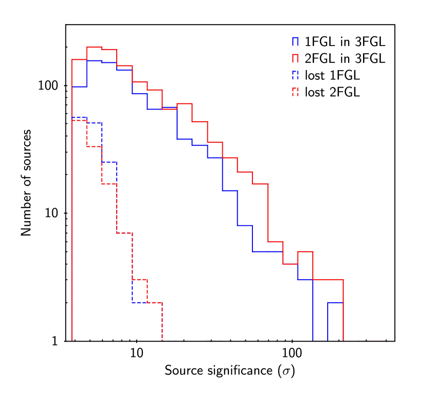
A comparison of the source significances of the ‘lost’ sources with those in the 3FGL catalog shows that (Figure 21) in the latter we have not lost highly-significant sources. The peaks of the source significance distributions for all the sources of the FGL catalogs (not shown in the Figure 21) have shifted from 4–6 for 1FGL to 4–5 for 2FGL and 3FGL.

The power-law indices of high-Galactic latitude () ‘lost’ sources with power-law spectral type tend to be softer than average for their catalogs (Figure 22).
The numbers of associated sources among the 0FGL, 1FGL, and 2FGL catalogs, and the 3FGL catalog do depend on the criteria used to define spatial coincidence (Eq. 4).
The numbers of 1FGL – 3FGL, 2FGL – 3FGL and 1FHL – 3FGL associated sources increase if we use as association criterion161616Assuming a Rayleigh distribution for the source angular separations, is evaluated using
.. The 193 additional associations (listed in Table 11 and corresponding 0FGL, 1FGL, 1FHL tables in the column ‘3FGL ()’) represent about 5% of the 0FGL, 1FGL, 2FGL, and 1FHL sources, as expected when passing from to .
Furthermore, the improved model of the Galactic diffuse emission (§ 2.3) used to build the 3FGL catalog together with the expected increase of the signal-to-noise ratio due to the use of 48 months of data, allowed us to obtain better localizations of the sources at positions that might be outside the 95% confidence error regions reported in the 0FGL, 1FGL, or 2FGL catalogs. Indeed, about half of the 193 additional associations concern sources located along the Galactic plane.
Also, in the 1FGL catalog the positions of sources associated with the LAT-detected pulsars and X-ray binaries are the high-precision positions of the identified counterparts. (These sources can be easily recognized because they have null values in the localization parameters reported in the 1FGL catalog.) Not all of these associations appear in the 3FGL catalog because they cannot be associated using , but those that can be associated using are listed in Table 11 (and corresponding 0FGL, 1FGL, and 1FHL tables).
To study a possible reason for 0FGL, 1FGL, 2FGL, and 1FHL sources to disappear in the 3FGL catalog, we have compared the they had when published in their respective catalogs with their values in the 3FGL analysis. The 3FGL catalog was built, in fact, starting from 4003 seeds with in the analysis (§ 3.1). The final analysis, which did not change the positions of the seeds, resulted in the 3033 sources with that make up the 3FGL catalog. Therefore, possibly many seeds did not reach the threshold but can be associated with 0FGL, 1FGL, 2FGL, and 1FHL sources (using ). These sources, marked with ‘T’ (for ‘’) in the ‘3FGL Seed’ column of the Table 11, can be considered to be previously confirmed sources whose significance dropped below the threshold, either as a result of time variability, changes in the model or in the catalog analysis procedure for Galactic diffuse emission. Finally we looked for those ‘lost’ sources whose distances from an extended 3FGL source are less than , and these are flagged with ‘E’ in the column ‘Flag’ of Table 11.
4.2.4 Step-by-step from 2FGL to 3FGL
In order to understand the improvements of the 3FGL analysis with respect to 2FGL, we have considered the effects of changing the analysis, the data set, and the diffuse emission model without changing the time range (i.e., leaving it as two years). To that end we started with the 2FGL catalog and changed each of those three elements in sequence and compared each intermediate result with the previous one.
-
•
The main difference between the analyses is the / handling (§ 3.2). The comparison showed that using identical isotropic diffuse spectra for and events in 2FGL resulted in underestimating the low-energy fluxes of high-latitude sources. As a consequence, the corrected analysis leads to larger values, higher photon fluxes, softer spectra, and smaller curvatures than in 2FGL. The effects are small on the scale of individual sources but collectively obvious. Quantitatively, the average difference in spectral index induced by this change was measured to be +0.05. Because that effect is due to the background, it is at the same level in units () for faint and bright sources.
-
•
Changing data from Pass 7 (2FGL) to Pass 7 reprocessed (3FGL) results in somewhat larger , harder sources and more curved spectra (but no change of integral flux on average). The average difference in spectral index is 0.03. This goes in the opposite direction to (and therefore partly offsets) the difference due to the separate / handling. However the dependence on flux is not the same. The reprocessing affects essentially all spectral indices and curvatures equally in absolute terms.
-
•
Finally, changing the model for Galactic diffuse emission from gal_2yearp7v6_v0 used in 2FGL to gll_iem_v05_rev1 results in smaller , lower fluxes and less curved spectra (but no change of spectral index on average). Like the first point above, this background-related effect is smaller in absolute (curvature) or relative (flux) terms for brighter sources.
In conclusion, to first order the resulting net changes are not very large, consistent with the general comparison between 3FGL and 2FGL at the beginning of this section. The 3FGL sources tend to be less curved than 2FGL ones. In particular, there are fewer pathological very strongly curved sources (with and Flag 12 set) in 3FGL (41) than in 2FGL (64) even though there are more LogParabola spectra in 3FGL (395) than in 2FGL (336) because of the better statistics.
| 2FGL | 2FGL Assoc.(a)(a)footnotemark: | (a)(a)footnotemark: | (a)(a)footnotemark: | (a)(a)footnotemark: | (a)(a)footnotemark: | Spec.(a)(a)footnotemark: | Var(a)(a)footnotemark: | 3FGL(b)(b)footnotemark: | 3FGL(c)(c)footnotemark: | (d)(d)footnotemark: | 3FGL(e)(e)footnotemark: | Flags(f)(f)footnotemark: | |
|---|---|---|---|---|---|---|---|---|---|---|---|---|---|
| (deg) | (deg) | (deg) | Index | 90% | () | () | (deg) | Seed | |||||
| J0004.2+2208 | 108.732 | 39.430 | 0.194 | 5.4 | 2.49 | F | T | ||||||
| J0011.3+0054 | PMN J0011+0058 | 102.317 | 60.352 | 0.223 | 6.2 | 2.43 | T | F | |||||
| J0013.8+1907 | GB6 J0013+1910 | 110.786 | 42.858 | 0.160 | 4.1 | 2.06 | T | ||||||
| J0014.30509 | 99.374 | 66.312 | 0.169 | 4.2 | 2.45 | F | J0014.30455 | 0.322 | 0.725 | T | F | ||
| J0118.64631 | 289.226 | 69.872 | 0.134 | 4.5 | 1.78 | F | |||||||
| J0124.62322 | 188.135 | 81.611 | 0.113 | 7.5 | 2.31 | F | J0123.72312 | 0.217 | 1.225 | S,F | |||
| J0128.0+6330 | 126.998 | 0.922 | 0.255 | 5.0 | 2.57 | F | J0128.4+6257 | 0.432 | 1.262 | F | |||
| J0129.4+2618 | 133.451 | 35.784 | 0.333 | 4.9 | 2.56 | F | J0127.9+2551 | 0.813 | 0.707 | T | |||
| J0158.6+8558 | 124.201 | 23.262 | 0.180 | 4.2 | 2.52 | F | J0145.6+8600 | 0.334 | 0.691 | T | |||
| J0214.5+6251c | 132.251 | 1.495 | 0.134 | 4.1 | 2.26 | F | c,F | ||||||
| J0218.7+6208c | 132.937 | 0.975 | 0.078 | 10.5 | 2.77 | F | J0217.3+6209 | 0.208 | 0.753 | T | S,c,F | ||
| J0219.11725 | 1RXS J021905.8172503 | 191.883 | 67.564 | 0.148 | 4.3 | 1.92 | F | T | |||||
| J0221.3+6025c | 133.810 | 0.528 | 0.110 | 4.6 | 2.45 | F | J0221.1+6059 | 0.391 | 1.451 | c,F | |||
| J0221.4+6257c | 132.962 | 1.856 | 0.118 | 9.5 | 2.64 | F | J0223.5+6313 | 0.316 | 1.11 | T | S,c,F | ||
| J0227.2+6029c | 134.471 | 0.220 | 0.097 | 6.1 | 2.38 | F | c,F |
This table is published in its entirety in the electronic edition of the Astrophysical Journal Supplements. A portion is shown here for guidance regarding its form and content.
Similar tables are available, only in the electronic edition, for lost 0FGL, lost 1FGL, and lost 1FHL sources.
5 Source Association and Identification
5.1 Firm Identifications
As with the 2FGL and earlier LAT catalogs, we retain the distinction between associations and firm identifications. Although many associations that we list between LAT sources and potential counterparts at other wavelengths, particularly those for AGN, have very high probability of being true, a firm identification, shown in the catalog by capitals in the Class column in Table 6, is based on one of three criteria:
-
1.
Periodic Variability. Pulsars are the largest class in this category. All PSR labels indicate that pulsed rays have been seen from the source with a probability of the periodicity occurring by chance of less than 10-6. Pulsars detected in blind searches of LAT data are indicated as ‘LAT PSR’ in the ‘ID or Assoc.’ column of Table 4; the other PSR detections are based on folding with radio or X-ray ephemerides (see Abdo et al., 2013). A similar chance probability requirement applies to the other set of periodic sources, the high-mass binaries (HMB). Three of these are included in the catalog: LS I +61 303 (Abdo et al., 2009c), LS 5039 (Abdo et al., 2009e), and 1FGL J1018.65856 (Corbet et al., 2011). Although not quite meeting the same chance probability, another binary (BIN) is included as an identification: Eta Carinae (Reitberger et al., 2012, 2014).
-
2.
Spatial Morphology. Spatially extended sources whose morphology can be related to extent seen at other wavelengths include SNR, PWNe, and galaxies, as described in § 3.4. The Centaurus A lobes and core are both marked as identified, because they are part of the same extended source, although the core itself does not show spatial extent. Although individual molecular clouds could in principle be included in this list, the catalog construction incorporates most known clouds into the diffuse model, and so no sources of this type are identified in the catalog.
-
3.
Correlated Variability. Variable sources, primarily AGN, whose -ray variations can be matched to variability seen at one or more other wavelengths, are considered to be firm identifications. Although some cases are well documented, such correlated variability is not always easily defined. We conservatively require data in more than two energy bands for comparison. Finding a blazar to have a high X-ray flux at the same time as a -ray flare, for example, does not qualify if there is no long-term history for the X-ray emission. We include those sources whose variability properties are documented either in papers or with Astronomer’s Telegrams171717See http://www.astronomerstelegram.org.. This list does not represent the result of a systematic study. Ongoing work will undoubtedly enlarge this list. The one Galactic source identified in this way is nova V407 Cygni (Abdo et al., 2010h). Similarly short duration tangent gamma-ray emission observed from the classical novae, V959 Mon 2012 and V1324 Sco 2012, were not detected in the 4-year integrated analysis in the 3FGL (Ackermann et al., 2014a).
We include one exception to these rules. The Crab PWN is listed as a firm identification even though it does not meet any of these criteria. The well-defined energy spectrum, distinct from the Crab pulsar spectrum and matching spectra seen at both lower and higher energies provides a unique form of identification (Abdo et al., 2010e).
In total, we firmly identify 238 out of the 3033 3FGL sources. Among those, 143 are pulsars, 66 are active galactic nuclei (BCU, BLL, FSRQ, NLSY1, or RDG) 12 are SNR, 4 are binaries (BIN or HMB), 9 are PWN, 2 are normal galaxies, 1 is a massive star-forming region, and 1 is a nova (Table 6).
5.2 Automated Source Associations
Our approach for automated source association closely follows that used for the 2FGL, and details of the method are provided in Abdo et al. (2010d, 1FGL) and Nolan et al. (2012, 2FGL).
In summary, we use a Bayesian approach that trades the positional coincidence of possible counterparts with 3FGL sources against the expected number of chance coincidences to estimate the probability that a specific counterpart association is indeed real (i.e., a physical association). As for 1FGL and 2FGL, we retain counterparts as associations if they reach a posterior probability of at least 80%. We apply this method to a set of counterpart catalogs for which we calibrate the prior source association probabilities using Monte Carlo simulations of fake 3FGL catalogs.
Table 12 lists the catalogs used in the automatic association procedure, organized into four categories: (1) known or plausible -ray-emitting source classes, (2) surveys at other frequencies, (3) GeV sources, and (4) identified -ray sources. The first category allows us to assign 3FGL sources to object classes, while the second category reveals multiwavelength counterparts that may suggest the possible nature of the associated 3FGL sources. The third category allows assessment of former GeV detections of 3FGL sources, and the fourth keeps track of all firm identifications (cf. § 5.1). For this last category we claim associations based on the spatial overlap of the true counterpart position with the 3FGL confidence error ellipse.
With respect to 2FGL, we updated all catalogs for which more comprehensive compilations became available. As for 1FGL and 2FGL, we separately consider energetic and nearby pulsars, with spin-down energy flux erg kpc-2 s-1. We also consider millisecond pulsars (MSPs) separately. For spin period (s) and spin-down rate , we define MSPs as pulsars satisfying .
Catalogs indicated with an asterisk in Table 12 have source location uncertainties greater than those for the 3FGL sources. Catalogs indicated with a dagger have extended sources, with sizes greater than the source location uncertainty regions for 3FGL. For these catalogs we cannot apply the Bayesian association method. For the former catalogs we base associations on overlap of the 95% confidence error radii. For the latter, we require overlap between the extended source and the 95% confidence radius (semi-major axis) of the 3FGL source. These approaches are much less reliable than the Bayesian associations, so we do not claim any associations based on overlap in our final catalog. We record, however, any spatial overlap with a TeV source in the FITS file version of the catalog, and use a special flag in our catalog (TEVCAT_FLAG), distinguishing point-like (P, angular diameter ) from extended (E) TeV counterparts (see App. B). We furthermore list all unassociated 3FGL sources that are spatially overlapping with SNRs or PWNe in Table 7.
| Name | Objectsaac indicates that based on the region of the sky the source is considered to be potentially confused with Galactic diffuse emission.All the values reported in these columns are from the 2FGL catalog. | Ref. |
|---|---|---|
| High pulsars | 213 | Manchester et al. (2005)bbe indicates a source that was modeled as spatially extended.Name of the 3FGL source associated with the 2FGL source with positional coincidence evaluated using . |
| Other normal pulsars | 1657 | Manchester et al. (2005)bbhttp://www.atnf.csiro.au/research/pulsar/psrcat |
| Millisecond pulsars | 137 | Manchester et al. (2005)bbhttp://www.atnf.csiro.au/research/pulsar/psrcat |
| Pulsar wind nebulae | 69 | Collaboration internal |
| High-mass X-ray binaries | 114 | Liu et al. (2006) |
| Low-mass X-ray binaries | 187 | Liu et al. (2007) |
| Point-like SNR | 157 | Green (2009) |
| Extended SNR† | 274 | Green (2009) |
| O stars | 378 | Maíz-Apellániz et al. (2004) |
| WR stars | 226 | van der Hucht (2001) |
| LBV stars | 35 | Clark et al. (2005) |
| Open clusters | 2140 | Dias et al. (2002) |
| Globular clusters | 160 | Harris (1996) |
| Dwarf galaxies† | 100 | McConnachie (2012) |
| Nearby galaxies | 276 | Schmidt et al. (1993) |
| IRAS bright galaxies | 82 | Sanders et al. (2003) |
| BZCAT (Blazars) | 3060 | Massaro et al. (2009) |
| BL Lac | 1371 | Véron-Cetty & Véron (2010) |
| AGN | 10066 | Véron-Cetty & Véron (2010) |
| QSO | 129,853 | Véron-Cetty & Véron (2010) |
| Seyfert galaxies | 27651 | Véron-Cetty & Véron (2010) |
| Radio loud Seyfert galaxies | 29 | Collaboration internal |
| 1WHSP | 1000 | Arsioli et al. (2014) |
| WISE blazar catalog | 7855 | D’Abrusco et al. (2014) |
| NRAO VLA Sky Survey (NVSS)ccSources without a counterpart in 3FGL catalog, at the level of overlapping 95% source location confidence contours. These sources are discussed in Table 10.Closest 3FGL source having a distance from the position of the 2FGL source. | 1,773,484 | Condon et al. (1998) |
| Sydney University Molonglo Sky Survey (SUMSS)ccAll-sky surveys used only in the Likelihood Ratio method, see § 5.2.1 | 211,050 | Mauch et al. (2003) |
| Parkes-MIT-NRAO surveyccAll-sky surveys used only in the Likelihood Ratio method, see § 5.2.1 | 23277 | Griffith & Wright (1993) |
| CGRaBS | 1625 | Healey et al. (2008) |
| CRATES | 11499 | Healey et al. (2007) |
| VLBA Calibrator Source List | 5776 | http://www.vlba.nrao.edu/astro/calib/vlbaCalib.txt |
| ATCA 20 GHz southern sky survey | 5890 | Murphy et al. (2010) |
| ATCA follow up of 2FGL unassociated sources | 424 | Petrov et al. (2013) |
| ROSAT All Sky Survey (RASS) Bright and Faint Source CatalogsccAll-sky surveys used only in the Likelihood Ratio method, see § 5.2.1 | 124,735 | Voges et al. (1999),ddIn this column is reported the angular separation () between the 2FGL source and the 3FGL sources associated using or the closest 3FGL source. |
| 58 months BAT catalog | 1092 | Baumgartner et al. (2010) |
| 4th IBIS catalog | 723 | Bird et al. (2010) |
| 1st AGILE catalog∗ | 47 | Pittori et al. (2009) |
| 3rd EGRET catalog∗ | 271 | Hartman et al. (1999) |
| EGR catalog∗ | 189 | Casandjian & Grenier (2008) |
| 0FGL list∗ | 205 | Abdo et al. (2009d, 0FGL) |
| 1FGL catalog∗ | 1451 | Abdo et al. (2010d, 1FGL) |
| 2FGL catalog∗ | 1873 | Nolan et al. (2012, 2FGL) |
| 1FHL catalog∗ | 514 | Ackermann et al. (2013a, 1FHL) |
| TeV point-like source catalog∗ | 82 | http://tevcat.uchicago.edu/ |
| TeV extended source catalog† | 66 | http://tevcat.uchicago.edu/ |
| LAT pulsars | 147 | Collaboration internal |
| LAT identified | 137 | Collaboration internal |
5.2.1 Active Galactic Nuclei associations
AGN, and in particular blazars, are the largest class of associated sources in 3FGL at high Galactic latitudes.
In 3LAC, as in the Second LAT Catalog of AGN (2LAC, Ackermann et al., 2011b), we added another association method to the automatic one described above. This is the Likelihood Ratio method (LR), frequently used to assess identification probabilities for radio, infrared and optical sources (e.g., de Ruiter et al., 1977; Prestage & Peacock, 1983; Sutherland & Saunders, 1992; Lonsdale et al., 1998; Masci et al., 2001; Ackermann et al., 2011b). It is based on uniform surveys in the radio and in X-ray bands, enabling us to search for possible counterparts among the faint radio and X-ray sources. The LR method makes use of counterpart densities (assumed spatially constant over the survey region) through the relation and therefore the source flux. This approach has been already used in 2LAC and we refer the reader to § 3.2 of that paper for a comprehensive description of the method, which computes the probability that a suggested association is the ‘true’ counterpart.181818We note that the implementation of the LR method for the 2LAC associations was plagued with an error in the management of the sky coordinate precession that affected some of the associations. These false associations were also included in the active galaxy associations in 2FGL. The error has been fixed and the 2FGL associations re-derived. The corrected 2FGL catalog file has been delivered to the FSSC for distribution. In the present work, comparisons with 2FGL findings are based on this corrected set of associations.
A source is considered as a likely counterpart of the -ray source if its reliability (see Eq. 4 in 2LAC) is greater than 0.8 in at least one survey.
In total, our automatic association procedure based on the Bayesian method finds 1663 3FGL sources that are associated with AGN while the LR-based association method finds 1340 3FGL sources. For 405 sources only the Bayesian method provides an association, and for 82 sources only the LR method does so.
Overall, 3FGL includes 1745 sources associated with AGN ( of all 3FGL sources) of which 1145 are blazars, 573 are candidate blazars, 15 are radio galaxies, 5 are Seyfert galaxies, and 3 are other AGN. The Seyfert galaxies are narrow-line Seyfert 1 galaxies that have been established as a new class of -ray active AGN (Abdo et al., 2009f).
Comparing to 2FGL we can make the following observations:
-
•
The 3FGL includes 610 more sources of AGN type than the 2FGL, i.e., a 76% increase. The fraction of new sources (not present in 2FGL) is slightly higher for hard-spectrum (i.e., 2.2) sources than for soft-spectrum ones (i.e., 2.2), 51% vs. 47% respectively, but the relative increase reaches 72% for very hard-spectrum (i.e., 1.8) sources. In the 3FGL, 477 counterparts are new (81 FSRQs, 146 BL Lacs, 240 candidate blazars of unknown type, 10 non-blazar objects); the other counterparts were present in previous AGN Fermi catalogs but not included in any of the 0FGL, 1FGL, or 2FGL catalogs for various reasons (e.g., the corresponding -ray sources were not associated with AGN, had more than one counterpart or were flagged in the analysis).
-
•
The fraction of counterparts of unknown type (named ‘bcu’) has increased notably between the two catalogs (from 20% to 28%). The number of these sources in the 3FGL has increased by more than a factor of 2.5 relative to that in the 2FGL, becoming almost equal to that of FSRQs. This increase is mainly due to the lower probability of having a published high-quality spectrum available for these fainter sources because of the lack of optical observing programs. In 3LAC, sources of the ‘bcu’ type have been divided into three sub-types depending of the multi-wavelength information available to characterize their ‘blazarness’. In this paper we do not propagate this sub-division and refer to the 3LAC for census.
-
•
The relative increase in ‘bcu’ drives a drop in the proportions of FSRQs and BL Lacs, which only represent 29% and 41% of the 3FGL respectively (38% and 48% for 2FGL). The relative increase in the number of sources with respect to 2FGL is 34% and 42% for FSRQs and BL Lacs respectively.
-
•
Out of 825 AGN in the 2FGL, a total of 68 are missing in the full 3LAC sample, most of them due to variability effects. A few others are present in 3FGL but with shifted positions, ruling out the association with their former counterparts.
5.2.2 Normal galaxies
The -ray emission of normal galaxies is powered by cosmic-ray interactions with interstellar gas and radiation. They are numerous but typically faint relative to active galaxies. The most luminous of the normal galaxies are starburst galaxies, which have very high densities of gas and massive star formation near their centers. Less distant are normal galaxies in the local group. As described above we searched for associations with sources in catalogs of nearby galaxies and IRAS bright galaxies (Table 12).
In the 3FGL catalog we do not find additional associations with normal galaxies relative to those reported already in 2FGL : starburst galaxies M82 (3FGL J0955.4+6940), NGC 253 (3FGL J0047.52516) NGC 1068 (3FGL J0242.70001), and NGC 4945 (3FGL J1305.44926), and local group galaxies LMC (3FGL J0526.66825e), M31 (3FGL J0042.5+4117), and the SMC (3FGL J0059.07242e).
Five sources in the 3FGL catalog lie within the extended source model for the LMC and are otherwise unassociated with counterparts at other wavelengths. These sources (3FGL J0456.26924, 3FGL J0524.56937, 3FGL J0525.26614, 3FGL 0535.36559, and 3FGL J0537.07113) are classified here as ‘gal’ based solely on the spatial coincidence with the LMC and their associations are listed as LMC field. Their particular natures remain uncertain.
5.2.3 Pulsars
Because pulsed emission can be such a clear signature, pulsars represent the largest class of firmly identified astrophysical objects in the 3FGL catalog. An extensive discussion of -ray pulsar properties is found in the Second Fermi Large Area Telescope Catalog of Gamma-ray Pulsars (Abdo et al., 2013, 2PC). The public catalog of LAT-detected pulsars is regularly updated191919See https://confluence.slac.stanford.edu/display/GLAMCOG/Public+List+of+LAT-Detected+Gamma-Ray+Pulsars.. At the time of the 3FGL association analysis, this catalog had 147 pulsars (Table 12). Only 137 of the LAT-detected pulsars have associations in the 3FGL catalog, however (Table 6). The missing ten did not reach the criterion based on their average fluxes. Three of these are PSR J07373039A (Guillemot et al., 2013), J1640+2224, and J17051906 (Hou et al., 2014), and the remaining seven are flagged in the 2PC ‘spectral results’ tables as being either too faint to fit, or requiring an on-peak analysis to obtain spectra.
5.2.4 Pulsar wind nebulae
In addition to the four pulsar wind nebulae found in 2FGL (Crab, Vela-X, MSH 1552, HESS J1825137), the 3FGL catalog includes seven new PWNe associations. Five of these are firm identifications because they are spatially extended LAT sources (see Table 1): HESS J1303631 (3FGL J1303.06312e), HESS J1616508 (3FGL J1616.25054e), HESS J1632478 (3FGL J1633.04746e), HESS J1837069 (3FGL J1836.50655e), and HESS J1841055 (3FGL J1840.90532e). The other two are positional associations with known PWNe: G279.835.8 (3FGL J0454.66825) and G0.130.11 (3FGL J1746.32859c).
5.2.5 Globular clusters
Two globular cluster associations from the 2FGL catalog are not found in the 3FGL catalog:
-
1.
2FGL J1727.10704, previously associated with IC 1257, is found as 3FGL J1727.60654. This source is not formally associated with the globular cluster.
-
2.
2FGL J1824.82449, which was associated with NGC 6626, has been firmly identified as PSR J18242452A (Johnson et al., 2013). Its catalog listing is 3FGL J1824.62451.
The number of globular clusters associated with LAT sources does continue to grow. New associations are NGC 2608 (3FGL J0912.26452), NGC 6316 (3FGL J1716.62812), NGC 6441 (3FGL J1750.23704), NGC 6541 (3FGL J1807.54343), NGC 6717 (3FGL J1855.12243), and NGC 6752 (3FGL J1910.76000). NGC 6752 had previously been noted as a likely LAT source by Tam et al. (2011b).
5.2.6 Supernova remnants
Twelve SNRs are firmly identified in the 3FGL catalog as spatially extended sources (see Table 1). Six had previously appeared in the 2FGL catalog: IC 443, W28, W30, W44, W51C, and the Cygnus Loop. Additions are: S147 (3FGL J0540.3+2756e, Katsuta et al., 2012), Puppis A (3FGL J0822.64250e, Hewitt et al., 2012), Vela Jr. (3FGL J0852.74631e, Tanaka et al., 2011), RX J1713.73946 (3FGL J1713.53945e, Abdo et al., 2011d), Gamma Cygni (3FGL J2021.0+4031e, Lande et al., 2012), and HB21 (3FGL J2045.2+5026e, Reichardt et al., 2012; Pivato et al., 2013).
Additionally we consider eleven unresolved 3FGL sources as being confidently associated with SNRs, based on individual studies of these SNRs in LAT data (see Ferrand & Safi-Harb, 2012, and references therein)202020http://www.physics.umanitoba.ca/snr/SNRcat/. These are given the ‘snr’ designator (Table 6). The 2FGL sources that were designated ‘snr’ have been added to the ‘spp’ class in 3FGL. Many of the 68 SNR or PWNe in this table are spatially extended sources at other wavelengths, and therefore the chance probability of an overlap with a LAT source is non-negligible. As for previous LAT catalogs, we encourage great care in any analysis using these potential associations.
5.2.7 Binaries
Three HMB sources that appeared in 2FGL are also found in 3FGL: LS I +61 303 (3FGL J0240.5+6113), 1FGL J1018.65856 (3FGL J1018.95856), and LS 5039 (3FGL J1826.21450). All were firmly identified by binary periodicity. We note that each of the three is a TeV emitter but that the two other binary systems that have been detected in the TeV energy regime, HESS J0632057 and PSR B125963, do not have counterparts in 3FGL. PSR B125963/LS 2883 is a bright LAT source during a small part of the 3.4-year binary period following periastron (Tam et al., 2011a; Abdo et al., 2011a). HESS J0632057 has not been detected at all.
A fourth HMB from 2FGL, Cygnus X3 (2FGL J2032.1+4049) does not appear in 3FGL. It is an intermittent LAT source and was not active enough averaged over the four years of this catalog to produce a significant detection. Eta Carinae, which appeared in 2FGL as a possible massive star association, is included as 3FGL J1045.15941, identified as a binary system. The LAT data exhibit the known 5.5-year binary period (Reitberger et al., 2012, 2014). Although listed in the catalog as a nova, V407 Cygni is also a binary system. Its flaring activity in 2010 (Abdo et al., 2010h) was bright enough that it appears as 3FGL J2102.3+4547.
5.2.8 Multiwavelength associations
In addition to the catalogs of classified sources, we also searched for associations with catalogs of radio and TeV sources. Our association procedure for AGN heavily relies on associations with radio sources as most of the -ray emitting AGN are bright sources of radio emission (see § 5.2.1). In fact, essentially all of the radio associations we find have been classified subsequently as AGN.
We did not search for general associations with infrared, optical, or soft X-ray catalogs. Within the LAT source error regions we would find multiple potential counterparts, most of which necessarily would be due to chance, since many of the sources in these catalogs are thermal in nature. We included, however, the hard X-ray catalogs INTEGRAL-IBIS and Swift-BAT, and blazar candidates extracted from the infrared WISE catalog (D’Abrusco et al., 2014) in the automated association pipeline. These data, when included in a study of the spectral energy distributions to evaluate their synchrotron peak frequencies and general behaviors, help in understanding the natures of the candidate counterparts. This was done especially for all the sources classified as bcu/BCU and agn.
5.2.9 Statistics of association results
In total we find that 1976 of the 3033 sources in the 3FGL catalog (59%) have been associated with at least one non-GeV -ray counterpart by the automated procedures. Table 13 summarizes the association results.
| Category | 0FGL | 1FGL | 2FGL | 1FHLaaNumber of objects in the catalog. | 3FGL | |
|---|---|---|---|---|---|---|
| Total | 205 | 1451 | 1873 | 514 | 3033 | |
| Associated | 168 | 821 | 1224 | 449 | 2023 | |
| Unassociated | 37 | 630 | 649 | 65 | 1010 | |
| New -ray sourcesbbNon-overlapping 95% source location confidence contours compared to previous LAT catalogs, at the level of overlapping 95% source location confidence contours. | - | 1265 | 762 | 52 | 1312 | |
| Sources associated with former LAT detections | - | 186 | 1111 | 462 | 1721 | |
| Sources associated with former GeV detectionsccH̱ere only the 1AGL, 3EG, and EGR catalogs are considered. | 74 | 162 | 170 | 4 | 206 | |
| Firmly identified sources | 31 | 65 | 124 | 60 | 238 | |
| Sources associated with at least one object of known type | 153 | 623 | 952 | 385 | 1398 | |
| Sources which have counterparts only in the multiwavelength catalogs | - | 92 | 214 | 58 | 576 |
5.3 GeV and TeV Source Associations
Through 2014 August, 155 flaring Fermi-LAT sources were detected and promptly reported in more than 249 Astronomer’s Telegrams212121https://www-glast.stanford.edu/cgi-bin/pub_rapid. Of these sources, six are not in 3FGL. For two of these the flaring state was detected outside the time interval covered by 3FGL: S5 1044+71 (a 2FGL source classified as an FSRQ) and PMN J16262426 (in the proximity of an unassociated 2FGL source flagged as potentially contaminated by the diffuse emission). The other four are Cyg X3 (an HMB associated with 2FGL J2032.1+4049; see § 5.2.7), CGRaBS J1848+3219 (an FSRQ associated with 2FGL J1848.6+3241), PKS 1124186 (an FSRQ associated with 2FGL J1126.61856) and PKS 2123463 (an FSRQ associated with 2FGL J2125.04632). The reason that these three FSRQs are missing from the 3FGL catalog is probably that they have average fluxes below the detection threshold.
Sources in 3FGL that are positionally associated with sources seen by the ground-based TeV telescopes are of particular interest for broad-band spectral studies. As for the 2FGL catalog we studied associations with the TeVCat222222http://tevcat.uchicago.edu compilation of sources detected by very-high-energy observatories. The energy threshold for TeVCat sources is not uniform, but it is typically greater than 100 GeV. We used a compilation of TeVCat sources prepared on 2014 October 27 that has 148 unique entries. This comprises the so-called “Default” and “Newly Announced” TeV catalogs. We note that, as in 1FGL and 2FGL, the “Galactic Centre Ridge” was not included for association purposes since it represents diffuse emission over an extended region along the Galactic plane (Aharonian et al., 2006).
This TeVCat compilation by its nature does not represent a complete survey, and our general statistical procedure for evaluating probabilities of chance association could not be applied. As for 2FGL we separately considered point-like and extended TeVCat sources (Table 12). For point-like sources the criterion for association was overlapping 95% source location regions (indicated by ‘P’ in the ‘TeV’ column of Table 4). For extended sources (LAT or TeVCat) the criterion was spatial overlap within their respective angular extents (indicated by ‘E’). We note that, in the literature, the shapes of the extended TeV sources are usually approximated to a circle or to an ellipse. For the purposes of our association pipeline, we imposed a circular geometry on all extended TeV sources, setting the radius to the length of the semi-major axis. In the case of TeV sources whose morphologies depart significantly from a simple ellipse or a circle, this simplification of their geometry could lead to missed 3FGL associations.
In total, 124 3FGL sources have TeV counterparts. Of the 148 TeV sources considered, 117 have 3FGL associations and, out of these, 6 TeV sources have multiple 3FGL associations. Five of these are extended TeV sources and one is the Crab, which is associated with both the synchrotron and the inverse-Compton Crab 3FGL sources (3FGL J0534.5+2201s/3FGL J0534.5+2201i). The TeV sources HESS J1018589, Westerlund 2, HESS J1458608 and MGRO J2019+37 have two 3FGL associations each while Westerlund 1 has three 3FGL associations.
We note that the TeV source HESS J1018589 has two components, denoted A (a point source) and B (extended emission). Of the two 3FGL associations, 3FGL J1018.95856, a LAT high-mass binary, lies closer to location A and 3FGL J1016.35858, a LAT pulsar, lies closer to location B.
Table 14 shows the associations between extended TeVCat sources and 3FGL catalog sources. Some of these, designated with e appended to their source names, were explicitly modeled as extended sources corresponding to H.E.S.S. sources (see § 3.4).
Out of the 58 TeV AGN, 57 have associated sources in 3FGL. Only HESS J1943+213, tentatively classified as a high-synchrotron peaked (HSP) blazar (HESS Collaboration, 2011; Leahy & Tian, 2012), does not have a 3FGL association. This presumed blazar is unique in the TeV sky in that it shines through the Galactic plane. We note that the VERITAS source VER J2016371 is positionally associated with 3FGL J2015.63709 although the VERITAS source is probably a PWN (Aliu et al., 2014) and the LAT source is associated with an FSRQ of unknown redshift.
The Milagro source, MGRO J203141, which comprises TeV J20324130, was also included as a separate source in the TeV list that was used to evaluate the associations with 3FGL because it is postulated that its emission is due to more than one source (Abdo et al., 2007). Due to the large extent of MGRO J203141 (, Abdo et al., 2012a), it has positional overlap with eight 3FGL sources in addition to 3FGL J2032.24126. We have listed just one LAT source 3FGL J2028.64110e, the Cygnus Cocoon, as being associated with MGRO J203141.
Due to its large extent (), the Milagro Geminga source (Abdo et al., 2009h) has positional overlap with two 3FGL sources, 3FGL J0633.91746 (the Geminga pulsar) and the unidentified source 3FGL J0626.81743. We have associated only the Geminga pulsar with the Milagro source. Abdo et al. (2009h) postulate that the Milagro emission could be due to a pulsar-driven wind associated with Geminga.
The TeV sources Boomerang and SNR G103.302.7 have positional overlap at TeV energies. They are each positionally coincident with the same two 3FGL sources, the unidentified source 3FGL J2225.8+6045 and the pulsar, 3FGL J2229.0+6114. We have associated SNR G103.302.7 with 3FGL J2225.86045 and Boomerang, classified as a PWN at TeV energies, with 3FGL J2229.0+6114, the LAT pulsar.
Relative to 2FGL eight TeV sources are newly associated with LAT sources. All but one of these sources (HESS J1641463) had already been detected at TeV energies when 2FGL and 1FHL were released. None of these eight sources, however, have counterparts in those catalogs:
-
1.
The H.E.S.S. Galactic Center source is associated with 3FGL J1745.62859c. The corresponding source 2FGL J1745.62858, had a large enough position offset that it was not considered associated with the TeV source. The Galactic center remains, however, a particularly complex region whose detailed study is beyond the scope of this paper.
-
2.
Three HSP blazars (SHBL J001355.9185406, 1ES 0229+200 and 1ES 0347121) are associated with 3FGL sources.
-
3.
The shell SNR Tycho is associated with the faint LAT source 3FGL J0025.7+6404. Although the center of the TeV emission is offset by from the LAT source, the relatively large uncertainty of the LAT position indicates sufficient positional overlap for association.
-
4.
The TeV PWN HESS J1809193 is another new TeV association in 3FGL. Discovered at TeV energies in 2007, it is a relatively bright TeV source with an integral flux 14% that of the Crab Nebula in the same energy band (Aharonian et al., 2007).
-
5.
The unidentified TeV sources HESS J1626490 and HESS J1641463 are also new TeV associations for 3FGL.
Thirty-one TeV sources have no counterparts in 3FGL; one of these, the unidentified extended TeV source HESS J1857026, has an association in 1FHL (1FHL J1856.90252). It is the only TeV source to have a 1FHL association but none in 2FGL or 3FGL. The other TeV sources having no counterparts in 3FGL comprise 10 other unidentified TeV sources, 10 PWNe, 2 binaries, 4 shell-type SNRs, 2 SNR-molecular cloud associations, 1 composite SNR (i.e., 9 out of the 19 SNRs in TeVCat) and the HSP blazars discussed earlier.
We note that two TeV sources, HESS J1634472 and SNR W49B, were each associated with LAT sources in 2FGL and in 1FHL but do not have associations in 3FGL. A source coincident with W49B has been detected by the LAT, 3FGL J1910.90906 but this does not have positional overlap with the TeV detection of W49B.
The TeV source, HESS J1427608 had an association in 2FGL but was not associated with a LAT source in 1FHL and does not have an association in 3FGL.
| TeVCat Nameaa1FHL: 10 GeV | 3FGL Name |
|---|---|
| Boomerang | J2225.8+6045, J2229.0+6114 |
| CTA 1 | J0007.0+7302 |
| CTB 37A | J1714.53832 |
| Geminga | J0633.9+1746 |
| HESS J1018589 | J1016.35858, J1018.95856 |
| HESS J1303631 | J1303.06312e |
| HESS J1356645 | J1356.66428 |
| HESS J1458608 | J1456.76046, J1459.46053 |
| HESS J1503582 | J1503.55801 |
| HESS J1507622 | J1506.66219 |
| HESS J1614518 | J1615.35146e |
| HESS J1616508 | J1616.25054e |
| HESS J1626490 | J1626.24911 |
| HESS J1632478 | J1633.04746e |
| HESS J1640465 | J1640.44634c |
| HESS J1708443 | J1709.74429 |
| HESS J1718385 | J1718.13825 |
| HESS J1745303 | J1745.13011 |
| HESS J1800240 | J1800.82402 |
| HESS J1804216 | J1805.62136e |
| HESS J1809193 | J1810.11910 |
| HESS J1825137 | J1824.51351e |
| HESS J1834087 | J1834.50841 |
| HESS J1837069 | J1836.50655e |
| HESS J1841055 | J1840.90532e |
| HESS J1848018 | J1848.40141 |
| HESS J1858+020 | J1857.9+0210 |
| IC 443 | J0617.2+2234e |
| Kookaburra (Rabbit) | J1418.66058 |
| Kookaburra PWN | J1420.06048 |
| MGRO J1908+06 | J1907.9+0602 |
| MGRO J2019+37 | J2021.1+3651, J2017.9+3627 |
| MGRO J2031+41 | J2028.6+4110e |
| MSH 1552 | J1514.05915e |
| RX J0852.04622 | J0852.74631e |
| RX J1713.73946 | J1713.53945e |
| SNR G292.200.5 | J1119.16127 |
| Terzan 5 | J1748.02447 |
| TeV J2032+4130 | J2032.2+4126 |
| Vela X | J0833.14511e |
| VER J2019+407 | J2021.0+4031e |
| W 28 | J1801.32326e |
| W 51 | J1923.2+1408e |
| Westerlund 1 | J1648.34611, J1650.34600, |
| J1651.54626 | |
| Westerlund 2 | J1023.15745, J1024.35757 |
5.4 Properties of Unassociated Sources
Among the 3033 sources in the 3FGL catalog, 2033 have associations or identifications with known astrophysical objects. Although that number is greater than the total number of sources in the 2FGL catalog, 1010 (33%) of the 3FGL sources remain unassociated. Among these unassociated sources are many that were found in previous LAT catalogs, indicating that some persistent mysteries remain despite extensive efforts to find associations over the past few years. The continued prevalence of unassociated sources is expected, as the improvement in sensitivity with four years of flight data and improvements to the characterization of backgrounds have allowed Fermi-LAT to probe the -ray sky to unprecedented depths. As a result, direct comparison to previous releases is difficult.

The distribution of unassociated sources on the sky is compared in Figure 23 to the distribution of the associated sources. The plot reveals some important features that should be kept in mind when considering unassociated 3FGL sources. Of the 992 unassociated sources in the 3FGL, 334 fall within the Galactic plane (). This leaves 658 unassociated at sources for an average density of sources deg-2. While this density reflects the finite angular resolution and sensitivity of the instrument, some of the shortfall of associations is attributable to the fact that not all areas of the sky have been mapped uniformly at other wavelengths. For instance, a 3269 deg2 “overlap region” in the North Galactic Cap intensively covered by five radio catalogs GB6 (6 cm) FIRST (20 cm), NVSS (20 cm), WNSS (92 cm), and VLSSr (4 m), as well as by the Sloan Digital Sky Survey (SDSS DR9) optical survey (Kimball & Ivezić, 2008), contains only 31 unassociated sources. The corresponding density of unassociated sources is sources deg-2, nearly half of the overall average.
Within the Galactic plane, the unassociated source population is a combination of both Galactic and extragalactic source classes. Outside the plane, the LAT-detected AGN source density is 0.045 deg-2. By extrapolation, this implies that there should be 160 detectable AGN within the 10-degree band surrounding the Galactic plane (not accounting for incompleteness of AGN catalogs at low latitudes). Only 56 sources are associated with active galaxies in this region. At low latitudes the LAT detection threshold is higher, and catalogs of active galaxies are incomplete, but extrapolation from higher latitudes suggests that fewer than 100 of the unassociated sources in the region could be active galaxies.
Of the remaining unassociated sources, we expect most to be Galactic objects. If we use the fractions of Galactic associated sources in this latitude range as a guide, we find that nearly half should be pulsars (47%), and most of the remainder should be SNRs (44%), with only a small number of other Galactic sources (9%). These yet-to-be-detected pulsars may never be seen to pulse: part of the neutron star population will have magnetic and rotation axis orientations causing -ray emission to be spread over a large part of the rotation phase (Hou et al., 2014). This, combined with a low -ray flux in the presence of high background, renders blind periodicity searches insensitive to pulsations (Dormody et al., 2011). That many of these sources are likely to be previously undetected SNRs is also reasonable. Ackermann et al. (2012b) recognized that the distribution of unassociated LAT sources near the Galactic plane matched the scale height appropriate for Population I objects, such as the SNR parent population of massive stars.
It should be emphasized that a substantial fraction of the unassociated sources (40%) has at least one analysis flag set (§ 3.9). We find that 57% of the sources with at least one flag have , which reflects the complexity of the Galactic diffuse emission (§ 3.7.3 and § 3.8). Because of the difficulties in source detection against the bright diffuse background along the Galactic plane, unassociated sources with analysis flags set should be considered with caution. That difficulty is acute in the Galactic bulge (within of the Galactic center), in the Vela () and Cygnus () regions. The immediate vicinity of the Galactic center is particularly uncertain, with 7 sources within , on top of bright diffuse emission. We did not attempt in the framework of 3FGL to devise models dedicated to those regions, so the source positions and characteristics there are not as reliable as in the extragalactic sky.
We also note a number of clusters of unassociated sources, mostly near the Galactic plane. Obvious ones are near () = (133.5,+1), (340,2). Since there is no specific search for extended sources in 3FGL, many of those clusters are probably extended sources (supernova remnants, pulsar wind nebulae, star formation regions). The extended sources which are currently declared (§ 3.4) are all relatively bright, with a median significance of . This leaves a lot of room for fainter extended sources.
6 Galactic Source Number Counts
The 3LAC companion paper discusses briefly the source number counts of extragalactic sources. Here we address the Galactic source number counts, following the analysis for the 1FHL catalog which was based on the method described by Strong (2007), and which addressed energies above 10 GeV. For 3FGL we use energies above 1 GeV. Photon fluxes over that energy range ( of Table 4) are more accurate than over the full band, as explained in the 2FGL paper. The much larger number of sources in 3FGL compared to 1FHL means that the entire analysis is more robust.
The motivation for performing a Galactic source population analysis is firstly to obtain estimates of the global source characteristics, i.e., space density and luminosity function, secondly to estimate the contribution from sources below the detection threshold to the Galactic ‘diffuse’ emission, and thirdly to generate templates of this emission, to be incorporated into diffuse emission models for future source catalogs. Source population analysis also puts the detected sources in the context of the total source content of the Galaxy.
The method is guided by properties of known sources such as pulsars but does not attempt physical modeling of the sources; the approach is essentially geometrical, nevertheless the analysis reveals the basic properties of the source population. We refer to the modeling of the source population(s) as population synthesis. Since the population synthesis includes all sources down to arbitrarily low flux levels (for a given model), it can also be used to study the flux limit of the actual catalog, and assess how the observed source number counts are affected by the detection procedure. This serves as a consistency check on other methods of assessing the detection threshold.
An essential principle is to use the fact that low-latitude sources probe the high-luminosity, low space densities at large distances, while the high-latitude sources constrain the low-luminosity, high space density nearby objects. This is because high-luminosity sources are rare but visible to large distances which are only sampled in the Galactic plane, while low-luminosity sources are common but only visible when nearby, so dominate outside the plane. These samples are complementary and allow the full luminosity function to be estimated.
6.1 Source Population Synthesis
The population synthesis and subsequent analysis is performed using the GALPLOT software, which is publicly available232323http://sourceforge.net/projects/galplot.. Let be the luminosity of a source in ph s-1 in some energy range. We use photon luminosities since they are most directly related to the detectability of sources and detection thresholds. The luminosity function at Galactocentric distance and distance from Galactic plane is the space density of sources per unit luminosity . The shape of the luminosity function is assumed independent of position, i.e., is separable in and . After Strong (2007) we assume that the luminosity function depends on luminosity as for and is zero outside these limits. The total space density of sources is , which we normalize to the value at . For a source of luminosity at distance the flux is . The differential source number counts are defined as sources per unit flux over the area of sky considered. At lower , both the luminosity function and the spatial boundaries influence . For this analysis the source fluxes are binned in log() so that the plotted distributions are proportional to ; we use 5 bins per decade of , appropriate to the statistics available. We use standard Monte Carlo techniques to sample throughout the Galaxy, using oversampling to reduce statistical fluctuations if necessary. We use the sources generated from such simulations to form simulated catalogs extending below the 3FGL flux limit and compare the flux distributions with the observations.
In the present work we do not explicitly account for the source detection efficiency in 3FGL, but simply compare the predictions with the data mindful of the range of the estimated detection threshold. Since the detection efficiency and threshold depend on direction, mainly because of the Galactic diffuse emission, and also exposure variations, accounting for this would require considerably more study than possible in the present work, and is not required for the scope here.
A large number of models was generated and compared with the data; for this paper we choose one reference model which is found to reproduce the data satisfactorily, but which is not unique. This suffices to illustrate plausible properties of the Galactic source population. A complete study of source number counts, optimizing the model over all parameters and considering spatial distributions and more sky regions, or using information about particular source classes, is beyond the present paper, and is foreseen in a future work.
6.2 Model and Comparison With Data
Our reference model for the luminosity function has kpc-3, and an dependence on luminosity in the range ph s-1 above 1 GeV. The luminosity law is discussed in Strong (2007); the chosen power-law index 1.8 is larger than expected for normal pulsars (1.5 or less) or MSPs, but here we wish to encompass both of these source types, and also other sources like SNR, with a single power-law function, for simplicity. This index is required to fit at both low and high latitudes; the steep slope ensures enough low-luminosity sources to match high-latitude number counts.
The distribution in Galactocentric distance is based on the model of Lorimer et al. (2006) for the distribution of pulsars, taken as representative of Galactic sources. We adopt an exponential scale height of 500 pc, guided by that of pulsars; the source number count distribution depends only weakly on the scale height. This distribution peaks near kpc and falls to zero at ; it was chosen for illustration and has not been optimized for the 3FGL source number counts. The spectrum of sources was taken as a power-law with exponential cutoff, index 1.4 and cutoff energy 3.2 GeV, with correlated dispersion in these parameters as found for pulsars. This is representative of pulsars but is not critical for this work since we use integral photon fluxes above 1 GeV as the basis for the analysis of . The spectrum is used here only when comparing with the spectrum of interstellar emission, to estimate the contribution of sources to the diffuse emission (section 6.3).
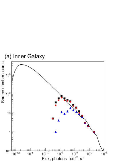
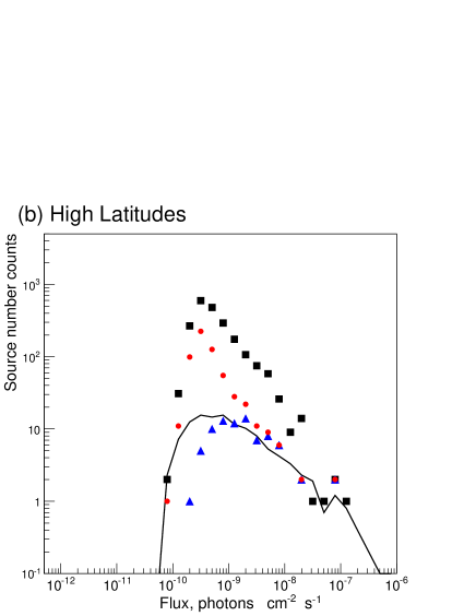

Figure 24 compares the simulated with the observed flux distributions of 3FGL sources at low latitudes in the inner Galaxy (, ) and high latitudes (), as well as for the full sky for reference. The predictions agree reasonably with Galactic plus unassociated sources at low latitudes, and with Galactic associated sources at high latitudes (where unassociated sources are probably mainly AGN). At high latitudes it is important that the model does not over-predict Galactic plus unassociated sources, and this condition is satisfied. The reference model is consistent with the low-latitude source number counts, having the observed dependence on flux above the source detection threshold; the slope reflects the spatial distribution (independent of the shape of the luminosity function) above ph cm-2 s-1, while the distributions for both the model and observed source number counts flatten at lower fluxes, following the luminosity function.
Some of the unassociated sources in the inner Galaxy may be AGN; using high-latitude AGN and unassociated sources (which are probably mainly AGN) and scaling by solid angle, we estimate about 30 AGN above the threshold for the inner Galaxy. This can be compared to 254 Galactic identified plus associated sources in the inner Galaxy for the same threshold, so that the AGN contribution is negligible, especially considering that most of these should be identified/associated AGN and hence excluded from our sample. For comparison there are 33 (identified/associated) AGN in this region, similar to our estimate from high latitudes, so the selection of Galactic classes certainly avoids the presence of more than a few AGN among the unassociated sources.
Pulsars, including MSPs, have a range of luminosities erg s-1 (Abdo et al., 2013), corresponding to about ph s-1 (taking a mean energy 2 GeV = erg). This is consistent with the range we have found from our analysis at low and high latitudes, although we are not assuming anything about the physical nature of the sources.
In this model there are sources in the Galaxy (in the luminosity range considered), with a total luminosity GeV of ph s-1, or about erg s-1. 3FGL contains about 266 Galactic sources (identified plus associated in Table 6) so that the LAT detects about 1% of the sources in the Galaxy; allowing for a significant number of unassociated sources at low latitudes being Galactic, a larger number is certainly included in 3FGL. Figure 24 shows that the distribution of simulated sources (in the reference model) continues down to fluxes 100 times below the detection threshold, the cutoff being due to the finite spatial extent of the Galaxy. The ratio of total flux below threshold to above threshold is about 0.25, which gives an estimate of the contribution of the undetected sources to the ‘diffuse’ emission (see below).
Using the work of Watters & Romani (2011) we can estimate the number of -ray pulsars in the Galaxy; they give a pulsar birthrate of 1 per 59 years, which corresponds to pulsars up to age 1 Myr. This is consistent with our model; we include other classes of sources, but this shows that our value is plausible.
6.3 Contribution of Undetected Sources to Diffuse Galactic Emission
Judging from the turnover in the inner Galaxy data, the detection threshold there is about ph cm-2 s-1, and we adopt this for the following estimates. For the inner Galaxy, the total flux from sources is ph cm-2 s-1, with ph cm-2 s-1 above threshold, ph cm-2 s-1 below threshold. So 20% of the total source flux is below threshold, and the ratio of flux below/above threshold is 25%. We can use the measured diffuse spectrum directly, comparing with the contribution from sources relative to interstellar emission: for the inner Galaxy as defined here, this gives 12% from sources above threshold, 3% from sources below threshold, at 1 GeV. These estimates are clearly model-dependent, in particular the adopted luminosity function gives a large number of low-luminosity sources, but they are certainly of the correct order, since varying the models within the range consistent with the data does not change the estimates greatly; details are beyond the scope of this paper.
For comparison with our estimates, Watters & Romani (2011) used physical modeling of young pulsars, and estimated their contribution to diffuse emission as 2.8%, however using all-sky averages and for only 6 months of LAT data taking. A study of the MSP contribution to the Galactic emission, for energies above 100 MeV, has been given by Grégoire & Knödlseder (2013); they find the contribution is at the few percent level.
Population synthesis can be used to estimate the increase in the number of sources with improved detection limits; in this model, reducing the threshold by a factor 2 would yield about twice as many sources at low latitudes.
Finally we consider the global picture. The luminosity of the interstellar emission from cosmic-ray interactions is about ph s-1 or erg s-1 for energies above 1 GeV (Strong et al., 2010) so that sources have about 20% of the interstellar luminosity. This is also an estimate of the contribution of all Galactic sources to the total Galactic -ray intensity, averaged over the sky.
7 Conclusions
The third Fermi LAT catalog is the deepest-yet in the 100 MeV–300 GeV energy range. The increased sensitivity relative to the 2FGL catalog is due to both the longer time interval (4 years vs. 2 years for 2FGL) and the use of reprocessed Pass 7 data, which provides a narrower PSF above 3 GeV. The 3FGL catalog also benefits from higher-level improvements in the analysis, including an improved model for Galactic diffuse emission, and a refined method for source detection.
The 3FGL catalog includes 3033 sources. The sources are detected () based on their average fluxes in the 4-year data set; 647 of the sources are found to be significantly variable on monthly timescales. We flag 78 (2.6%) of the sources as potentially being related to imperfections in the model for Galactic diffuse emission; the character c is appended to their names. An additional 572 (18.9%) are flagged in the catalog for less serious concerns, e.g., for the spectral model having a poor fit or for being close to a brighter source. Of the 3033 sources in the catalog, 238 (7.8%) are considered identified, based on correlated variability or (for 25 of the identified sources) correlated angular sizes with observations at other wavelengths. Of the remainder, we find likely lower-energy counterparts for 1786 sources (59.6%). The remaining 992 sources (32.7%) are unassociated.
The identified and associated sources in the 3FGL catalog include many Galactic and extragalactic source classes. The largest Galactic source class continues to be pulsars, with 1̱43 known -ray pulsars and 24 candidates. Other Galactic source classes have continued to grow; fifteen globular clusters are now associated with LAT sources. Our analysis of Galactic source counts, informed by a model for the luminosity function, suggests that at 1 GeV 3% of the Galactic diffuse emission is due to unresolved Galactic sources. Blazars remain the largest class of extragalactic source, with more than 1100 identified or associated with BL Lac or FSRQ active galaxies. Non-blazar classes of active galaxies are also found, including a Seyfert galaxy (Circinus galaxy), a compact steep spectrum radio source (3C 286) and several radio galaxies. The populations of active galaxies in 3FGL are considered in more detail in the companion 3LAC catalog.
References
- Abdo et al. (2012a) Abdo, A. A., Abeysekara, U., Allen, B. T., et al. 2012a, ApJ, 753, 159, (Milagro Cygnus)
- Abdo et al. (2009a) Abdo, A. A., Ackermann, M., Ajello, M., et al. 2009a, Phys. Rev. D, 80, 122004, (Earth limb)
- Abdo et al. (2009b) —. 2009b, ApJ, 706, L1, (W51C)
- Abdo et al. (2009c) —. 2009c, ApJ, 701, L123, (LS I +61 303)
- Abdo et al. (2009d) —. 2009d, ApJS, 183, 46, (0FGL)
- Abdo et al. (2009e) —. 2009e, ApJ, 706, L56, (LS 5039)
- Abdo et al. (2009f) —. 2009f, ApJ, 707, L142, (Radio-loud NLSy1)
- Abdo et al. (2009g) —. 2009g, Astroparticle Physics, 32, 193, (On-orbit calibration)
- Abdo et al. (2010a) —. 2010a, ApJ, 714, 927, (PSR B1509)
- Abdo et al. (2010b) —. 2010b, A&A, 523, A46, (SMC)
- Abdo et al. (2010c) —. 2010c, Science, 328, 725, (CenA lobes)
- Abdo et al. (2010d) —. 2010d, ApJS, 188, 405, (1FGL)
- Abdo et al. (2010e) —. 2010e, ApJ, 708, 1254, (Crab)
- Abdo et al. (2010f) —. 2010f, ApJ, 718, 348, (W28)
- Abdo et al. (2010g) —. 2010g, ApJ, 713, 146, (Vela X)
- Abdo et al. (2010h) —. 2010h, Science, 329, 817, (V407 Cyg)
- Abdo et al. (2010i) —. 2010i, Science, 327, 1103, (W44)
- Abdo et al. (2010j) —. 2010j, ApJ, 712, 459, (IC 443)
- Abdo et al. (2010k) —. 2010k, A&A, 512, A7, (LMC)
- Abdo et al. (2011a) —. 2011a, ApJ, 736, L11, (PSR B1259)
- Abdo et al. (2011b) —. 2011b, ApJ, 734, 116, (Sun)
- Abdo et al. (2011c) —. 2011c, Science, 331, 739, (Crab flares)
- Abdo et al. (2011d) —. 2011d, ApJ, 734, 28, (RX J1713)
- Abdo et al. (2012b) —. 2012b, ApJ, 758, 140, (Moon)
- Abdo et al. (2013) Abdo, A. A., Ajello, M., Allafort, A., et al. 2013, ApJS, 208, 17, (2PC)
- Abdo et al. (2007) Abdo, A. A., Allen, B., Berley, D., et al. 2007, ApJ, 664, L91, (Milagro survey)
- Abdo et al. (2009h) Abdo, A. A., Allen, B. T., Aune, T., et al. 2009h, ApJ, 700, L127, (Milagro Fermi)
- Acero et al. (2013) Acero, F., Ackermann, M., Ajello, M., et al. 2013, ApJ, 773, 77, (Fermi TeV PWN)
- Ackermann et al. (2012a) Ackermann, M., Ajello, M., Albert, A., et al. 2012a, ApJS, 203, 4, (Pass7)
- Ackermann et al. (2014a) —. 2014a, Science, 345, 554
- Ackermann et al. (2011a) Ackermann, M., Ajello, M., Allafort, A., et al. 2011a, Science, 334, 1103, (Cygnus X)
- Ackermann et al. (2011b) —. 2011b, ApJ, 743, 171, (2LAC)
- Ackermann et al. (2012b) —. 2012b, ApJ, 753, 83, (1FGL UNIDs)
- Ackermann et al. (2012c) —. 2012c, Astroparticle Physics, 35, 346, (Energy scale)
- Ackermann et al. (2013a) —. 2013a, ApJS, 209, 34, (1FHL)
- Ackermann et al. (2013b) Ackermann, M., Ajello, M., Asano, K., et al. 2013b, ApJS, 209, 11, (LAT GRBs)
- Ackermann et al. (2015) Ackermann, M., Ajello, M., Atwood, W. B., et al. 2015, ApJ, submitted (3LAC)
- Aharonian et al. (2005) Aharonian, F., Akhperjanian, A. G., Aye, K.-M., et al. 2005, A&A, 439, 1013
- Aharonian et al. (2008) Aharonian, F., Akhperjanian, A. G., Barres de Almeida, U., et al. 2008, A&A, 477, 353
- Aharonian et al. (2007) Aharonian, F., Akhperjanian, A. G., Bazer-Bachi, A. R., et al. 2007, A&A, 472, 489
- Aharonian et al. (2006) Aharonian, F., Akhperjanian, A. G., Bazer-Bachi, A. R., et al. 2006, Nature, 439, 695
- Ajello et al. (2012) Ajello, M., Allafort, A., Baldini, L., et al. 2012, ApJ, 744, 80
- Aliu et al. (2014) Aliu, E., Aune, T., Behara, B., et al. 2014, ApJ, 788, 78
- Allafort et al. (2013) Allafort, A., Baldini, L., Ballet, J., et al. 2013, ApJ, 777, L2
- Arsioli et al. (2014) Arsioli, B., Fraga, P., Giommi, P., Padovani, P., & Marrese, P. M. 2014, A&A, in press
- Atwood et al. (2009) Atwood, W. B., Abdo, A. A., Ackermann, M., et al. 2009, ApJ, 697, 1071
- Baumgartner et al. (2010) Baumgartner, W. H., Wayne, H., Tueller, J., Markwardt, C., & Skinner, G. 2010, in Bulletin of the American Astronomical Society, Vol. 42, AAS/High Energy Astrophysics Division #11, 675
- Bird et al. (2010) Bird, A. J., Bazzano, A., Bassani, L., et al. 2010, ApJS, 186, 1
- Bregeon et al. (2013) Bregeon, J., Charles, E., & Wood, M. 2013, ArXiv:1304.5456
- Casandjian & Grenier (2008) Casandjian, J.-M., & Grenier, I. A. 2008, A&A, 489, 849
- Casandjian & the Fermi LAT Collaboration (2015) Casandjian, J.-M., & the Fermi LAT Collaboration. 2015, ArXiv:1502.07210
- Clark et al. (2005) Clark, J. S., Larionov, V. M., & Arkharov, A. 2005, A&A, 435, 239
- Condon et al. (1998) Condon, J. J., Cotton, W. D., Greisen, E. W., Yin, Q. F., Perley, R. A., Taylor, G. B., & Broderick, J. J. 1998, AJ, 115, 1693
- Corbet et al. (2011) Corbet, R. H. D., Cheung, C. C., Kerr, M., et al. 2011, The Astronomer’s Telegram, 3221, 1
- D’Abrusco et al. (2014) D’Abrusco, R., Massaro, F., Paggi, A., Smith, H. A., Masetti, N., Landoni, M., & Tosti, G. 2014, ApJS, 215, 14
- de Palma et al. (2013) de Palma, F., Brandt, T. J., Johannesson, G., Tibaldo, L., & the Fermi LAT collaboration. 2013, ArXiv:1304.1395
- de Ruiter et al. (1977) de Ruiter, H. R., Arp, H. C., & Willis, A. G. 1977, A&AS, 28, 211
- Dias et al. (2002) Dias, W. S., Alessi, B. S., Moitinho, A., & Lépine, J. R. D. 2002, A&A, 389, 871
- Dormody et al. (2011) Dormody, M., Johnson, R. P., Atwood, W. B., Belfiore, A., Grenier, I. A., Johnson, T. J., Razzano, M., & Saz Parkinson, P. M. 2011, ApJ, 742, 126
- Ferrand & Safi-Harb (2012) Ferrand, G., & Safi-Harb, S. 2012, Advances in Space Research, 49, 1313
- Górski et al. (2005) Górski, K. M., Hivon, E., Banday, A. J., Wandelt, B. D., Hansen, F. K., Reinecke, M., & Bartelmann, M. 2005, ApJ, 622, 759
- Green (2009) Green, D. A. 2009, Bulletin of the Astronomical Society of India, 37, 45
- Grégoire & Knödlseder (2013) Grégoire, T., & Knödlseder, J. 2013, A&A, 554, A62
- Griffith & Wright (1993) Griffith, M. R., & Wright, A. E. 1993, AJ, 105, 1666
- Grondin et al. (2011) Grondin, M.-H., Funk, S., Lemoine-Goumard, M., et al. 2011, ApJ, 738, 42
- Guillemot et al. (2013) Guillemot, L., Kramer, M., Johnson, T. J., et al. 2013, ApJ, 768, 169
- Harris (1996) Harris, W. E. 1996, AJ, 112, 1487
- Hartman et al. (1999) Hartman, R. C., Bertsch, D. L., Bloom, S. D., et al. 1999, ApJS, 123, 79
- Healey et al. (2007) Healey, S. E., Romani, R. W., Taylor, G. B., Sadler, E. M., Ricci, R., Murphy, T., Ulvestad, J. S., & Winn, J. N. 2007, ApJS, 171, 61
- Healey et al. (2008) Healey, S. E., Romani, R. W., Cotter, G., et al. 2008, ApJS, 175, 97
- Helene (1983) Helene, O. 1983, Nuclear Instruments and Methods in Physics Research, 212, 319
- HESS Collaboration (2011) HESS Collaboration. 2011, A&A, 529, A49
- Hewitt et al. (2012) Hewitt, J. W., Grondin, M.-H., Lemoine-Goumard, M., Reposeur, T., Ballet, J., & Tanaka, T. 2012, ApJ, 759, 89
- Hou et al. (2014) Hou, X., Smith, D. A., Guillemot, L., et al. 2014, A&A, accepted
- Johannesson et al. (2013) Johannesson, G., Orlando, E., & the Fermi-LAT collaboration. 2013, ArXiv:1307.0197
- Johnson et al. (2013) Johnson, T. J., Guillemot, L., Kerr, M., et al. 2013, ApJ, 778, 106
- Katagiri et al. (2011) Katagiri, H., Tibaldo, L., Ballet, J., et al. 2011, ApJ, 741, 44
- Katsuta et al. (2012) Katsuta, J., Uchiyama, Y., Tanaka, T., et al. 2012, ApJ, 752, 135
- Kerr (2010) Kerr, M. 2010, PhD thesis, University of Washington, ArXiv:1101:6072
- Kimball & Ivezić (2008) Kimball, A. E., & Ivezić, Ž. 2008, AJ, 136, 684
- Lande et al. (2012) Lande, J., Ackermann, M., Allafort, A., et al. 2012, ApJ, 756, 5
- Leahy & Tian (2012) Leahy, D. A., & Tian, W. W. 2012, A&A, 539, A128
- Liu et al. (2006) Liu, Q. Z., van Paradijs, J., & van den Heuvel, E. P. J. 2006, A&A, 455, 1165
- Liu et al. (2007) —. 2007, VizieR Online Data Catalog, 346, 90807
- Lonsdale et al. (1998) Lonsdale, C., et al. 1998, in IAU Symposium, Vol. 179, New Horizons from Multi-Wavelength Sky Surveys, ed. B. J. McLean, D. A. Golombek, J. J. E. Hayes, & H. E. Payne (Dordrecht: Kluwer), 450
- Lorimer et al. (2006) Lorimer, D. R., Faulkner, A. J., Lyne, A. G., et al. 2006, MNRAS, 372, 777
- Maíz-Apellániz et al. (2004) Maíz-Apellániz, J., Walborn, N. R., Galué, H. Á., & Wei, L. H. 2004, ApJS, 151, 103
- Manchester et al. (2005) Manchester, R. N., Hobbs, G. B., Teoh, A., & Hobbs, M. 2005, AJ, 129, 1993
- Masci et al. (2001) Masci, F. J., Condon, J. J., Barlow, T. A., et al. 2001, PASP, 113, 10
- Massaro et al. (2009) Massaro, E., Giommi, P., Leto, C., Marchegiani, P., Maselli, A., Perri, M., Piranomonte, S., & Sclavi, S. 2009, A&A, 495, 691
- Mattox et al. (1996) Mattox, J. R., Bertsch, D. L., Chiang, J., et al. 1996, ApJ, 461, 396
- Mauch et al. (2003) Mauch, T., Murphy, T., Buttery, H. J., Curran, J., Hunstead, R. W., Piestrzynski, B., Robertson, J. G., & Sadler, E. M. 2003, MNRAS, 342, 1117
- McConnachie (2012) McConnachie, A. W. 2012, AJ, 144, 4
- Moskalenko & Strong (1998) Moskalenko, I. V., & Strong, A. W. 1998, ApJ, 493, 694
- Murphy et al. (2010) Murphy, T., Sadler, E. M., Ekers, R. D., et al. 2010, MNRAS, 402, 2403
- Nolan et al. (2012) Nolan, P. L., Abdo, A. A., Ackermann, M., et al. 2012, ApJS, 199, 31, (2FGL)
- Petrov et al. (2013) Petrov, L., Mahony, E. K., Edwards, P. G., Sadler, E. M., Schinzel, F. K., & McConnell, D. 2013, MNRAS, 432, 1294
- Pittori et al. (2009) Pittori, C., Verrecchia, F., Chen, A. W., et al. 2009, A&A, 506, 1563
- Pivato et al. (2013) Pivato, G., Hewitt, J. W., Tibaldo, L., et al. 2013, ApJ, 779, 179
- Prestage & Peacock (1983) Prestage, R. M., & Peacock, J. A. 1983, MNRAS, 204, 355
- Reichardt et al. (2012) Reichardt, I., de Oña-Wilhelmi, E., Rico, J., & Yang, R. 2012, A&A, 546, A21
- Reitberger et al. (2012) Reitberger, K., Reimer, O., Reimer, A., Werner, M., Egberts, K., & Takahashi, H. 2012, A&A, 544, A98
- Reitberger et al. (2014) Reitberger, K.,Reimer, A., Reimer, O., & Takahashi, H. 2014, A&A, in press
- Sanders et al. (2003) Sanders, D. B., Mazzarella, J. M., Kim, D.-C., Surace, J. A., & Soifer, B. T. 2003, AJ, 126, 1607
- Schmidt et al. (1993) Schmidt, K., Priebe, A., & Boller, T. 1993, Astronomische Nachrichten, 314, 371
- Strong (2007) Strong, A. W. 2007, Ap&SS, 309, 35
- Strong et al. (2010) Strong, A. W., Porter, T. A., Digel, S. W., Jóhannesson, G., Martin, P., Moskalenko, I. V., Murphy, E. J., & Orlando, E. 2010, ApJ, 722, L58
- Sutherland & Saunders (1992) Sutherland, W., & Saunders, W. 1992, MNRAS, 259, 413
- Tam et al. (2011a) Tam, P. H. T., Huang, R. H. H., Takata, J., Hui, C. Y., Kong, A. K. H., & Cheng, K. S. 2011a, ApJ, 736, L10
- Tam et al. (2011b) Tam, P. H. T., Kong, A. K. H., Hui, C. Y., Cheng, K. S., Li, C., & Lu, T.-N. 2011b, ApJ, 729, 90
- Tanaka et al. (2011) Tanaka, T., Allafort, A., Ballet, J., et al. 2011, ApJ, 740, L51
- Tavani et al. (2011) Tavani, M., Bulgarelli, A., Vittorini, V., et al. 2011, Science, 331, 736
- van der Hucht (2001) van der Hucht, K. A. 2001, New Astronomy Review, 45, 135
- Véron-Cetty & Véron (2010) Véron-Cetty, M.-P., & Véron, P. 2010, A&A, 518, A10
- Voges et al. (1999) Voges, W., Aschenbach, B., Boller, T., et al. 1999, A&A, 349, 389
- Watters & Romani (2011) Watters, K. P., & Romani, R. W. 2011, ApJ, 727, 123
Appendix A Diffuse model adjustments
 |

|
 |

|
 |

|
| Column | Format | Unit | Description |
|---|---|---|---|
| ROI_num | I | ROI number (cross-reference to main table) | |
| RAJ2000 | E | deg | Right Ascension of ROI center |
| DEJ2000 | E | deg | Declination of ROI center |
| GLON | E | deg | Galactic Longitude of ROI center |
| GLAT | E | deg | Galactic Latitude of ROI center |
| Radius | E | deg | ROI radius (unbinned mode) or half-side (binned mode) |
| PARNAMaaFrom http://tevcat.uchicago.edu. | E | Value of diffuse model parameter | |
| Unc_PARNAM | E | error on PARNAM |
In § 3.2 we noted that the diffuse emission model has three free parameters in each RoI. We report their values in the ROIs extension of the catalog (Table 15) and we show in Figure 25 how they vary over the sky. The first thing to notice is that the amplitude of the variations is relatively small. Overall the Galactic normalization does not vary by more than 20%, and in the Galactic plane (i.e., where it is the dominant component) it does not vary by more than 10%. The slope of the power-law correction does not exceed 0.1 (positive or negative) and inside the plane it does not exceed 0.05. The isotropic normalization does not vary by more than 40%, and outside the Galactic plane (i.e., where it is the dominant component) it does not vary by more than 20%. This indicates that the diffuse model is quite accurate. Nevertheless, the statistical precision of the data is so good that the deviations are formally very significant. Leaving those parameters free allows releasing some of the tension that exists locally between the data and the diffuse model.
At high latitudes (left-hand plots) the isotropic component is stable (as it should) but the Galactic normalization shows a clear North-South effect. The model is too high in the South but lacks emission in the North. The middle plot also indicates that the model is somewhat too hard particularly in the North. The group of points where the model is too hard in the South is around (RA,Dec) = (+10°,60°).
At low latitudes (right-hand plots) the error bars on the Galactic diffuse parameters are very small and the parameter values are very correlated between an RoI and its neighbor. This is because the distance between the centers of neighboring RoIs in the plane (a few degrees) is much smaller than their diameter (15 to 20°). The model appears to be too low and somewhat too hard East of the Galactic center (around longitude +35°) whereas it is too high and too soft just West of the Carina region (around longitude 80°). Outside those two regions the fitted Galactic model is very close to the original one. Inside the plane the isotropic component is a minor contributor and it tends to fluctuate a lot.
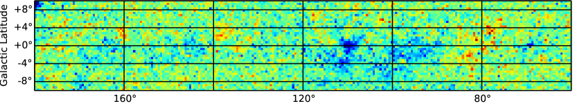

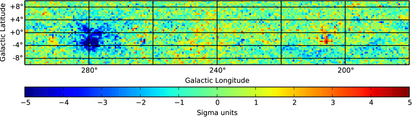
Figure 26 is another illustration of the same effect. It shows the residuals between the data and the full sky model (original diffuse model + 3FGL sources, without any free parameter), integrated from 100 MeV to 100 GeV. The figure is restricted to the Galactic plane because at the scale shown here ( pixels) nothing comes out clearly at high latitude. The units are sigma units (statistical deviations). The model was originally computed with 01 pixels in order to model the sources accurately. The main features are the data excess East of the Galactic center and the data deficit around 80°, which correspond to the features in Figure 25.
Appendix B Description of the FITS Version of the 3FGL Catalog
The FITS format version of the 3FGL catalog292929The file is available from the Science Support Center, http://fermi.gsfc.nasa.gov/ssc has four binary table extensions. The extension LAT_Point_Source_Catalog Extension has all of the information about the sources, including the monthly light curves (Table 16).
The extension Hist_Start lists the Mission Elapsed Time (seconds since 00:00 UTC on 2000 January 1) of the start of each bin of the monthly light curves. The final entry is the ending time of the last bin.
The extension GTI is a standard Good-Time Interval listing the precise time intervals (start and stop in MET) included in the data analysis. The number of intervals is fairly large because on most orbits (95 min) passes through the South Atlantic Anomaly (SAA), and science data taking is stopped during these times. In addition, data taking is briefly interrupted on each non-SAA-crossing orbit, as crosses the ascending node. Filtering of time intervals with large rocking angles, other data gaps, or operation in non-standard configurations introduces some more entries. The GTI is provided for reference and would be useful, e.g., for reconstructing the precise data set that was used for the 2FGL analysis.
The extension ExtendedSources (format unchanged since 2FGL) contains information about the 25 spatially extended sources that are modeled in the 3FGL catalog, including locations and shapes.
| Column | Format | Unit | Description |
|---|---|---|---|
| Source_Name | 18A | Official source name 3FGL JHHMM.m+DDMM | |
| RAJ2000 | E | deg | Right Ascension |
| DEJ2000 | E | deg | Declination |
| GLON | E | deg | Galactic Longitude |
| GLAT | E | deg | Galactic Latitude |
| Conf_68_SemiMajor | E | deg | Long radius of error ellipse at 68% confidence |
| Conf_68_SemiMinor | E | deg | Short radius of error ellipse at 68% confidence |
| Conf_68_PosAng | E | deg | Position angle of the 68% long axis from celestial North, |
| positive toward increasing RA (eastward) | |||
| Conf_95_SemiMajor | E | deg | Long radius of error ellipse at 95% confidence |
| Conf_95_SemiMinor | E | deg | Short radius of error ellipse at 95% confidence |
| Conf_95_PosAng | E | deg | Position angle of the 95% long axis from celestial North, |
| positive toward increasing RA (eastward) | |||
| ROI_num | I | ROI number (cross-reference to ROIs extension) | |
| Signif_Avg | E | Source significance in units (derived from Test Statistic) | |
| over the 100 MeV to 300 GeV band | |||
| Pivot_Energy | E | MeV | Energy at which error on differential flux is minimal |
| Flux_Density | E | cm-2 MeV-1 s-1 | Differential flux at Pivot_Energy |
| Unc_Flux_Density | E | cm-2 MeV-1 s-1 | error on differential flux at Pivot_Energy |
| Spectral_Index | E | Best fit photon number power-law index: for LogParabola spectra, | |
| index at Pivot_Energy; for PL(Super)ExpCutoff spectra, low-energy index | |||
| Unc_Spectral_Index | E | error on Spectral_Index | |
| Flux1000 | E | cm-2 s-1 | Integral photon flux from 1 to 100 GeV |
| Unc_Flux1000 | E | cm-2 s-1 | error on integral photon flux from 1 to 100 GeV |
| Energy_Flux100 | E | erg cm-2 s-1 | Energy flux from 100 MeV to 100 GeV obtained by spectral fitting |
| Unc_Energy_Flux100 | E | erg cm-2 s-1 | error on energy flux from 100 MeV to 100 GeV |
| Signif_Curve | E | Significance (in units) of the fit improvement between power-law | |
| and either LogParabola (for ordinary sources) or PLExpCutoff (for pulsars) | |||
| A value greater than 4 indicates significant curvature | |||
| SpectrumType | 18A | Spectral type (PowerLaw, LogParabola, PLExpCutoff, PLSuperExpCutoff) | |
| beta | E | Curvature parameter ( of Eq. 1) for LogParabola; NULL for other spectral types | |
| Unc_beta | E | error on for LogParabola; NULL for other spectral types | |
| Cutoff | E | MeV | Cutoff energy ( of Eq. 2) for PL(Super)ExpCutoff; NULL for other spectral types |
| Unc_Cutoff | E | MeV | error on cutoff energy for PL(Super)ExpCutoff; NULL for other spectral types |
| Exp_Index | E | Exponential index ( of Eq. 2) for PLSuperExpCutoff; NULL for other spectral types | |
| Unc_Exp_Index | E | error on exponential index for PLSuperExpCutoff; NULL for other spectral types | |
| PowerLaw_Index | E | Best fit power-law index; equal to Spectral_Index if SpectrumType is PowerLaw | |
| Flux30_100 | E | cm-2 s-1 | Integral photon flux from 30 to 100 MeV (not filled) |
| Unc_Flux30_100 | 2E | cm-2 s-1 | lower and upper error on integral photon flux from 30 to 100 MeV (not filled) |
| nuFnu30_100 | E | erg cm-2 s-1 | Spectral energy distribution between 30 and 100 MeV (not filled) |
| Sqrt_TS30_100 | E | Square root of the Test Statistic between 30 and 100 MeV (not filled) | |
| Flux100_300 | E | cm-2 s-1 | Integral photon flux from 100 to 300 MeV |
| Unc_Flux100_300 | 2E | cm-2 s-1 | lower and upper error on integral photon flux from 100 to 300 MeVaaTwo columns (value and error) for each diffuse model parameter. The parameter name is given by the PARNAM keyword in the extension header. |
| nuFnu100_300 | E | erg cm-2 s-1 | Spectral energy distribution between 100 and 300 MeV |
| Sqrt_TS100_300 | E | Square root of the Test Statistic between 100 and 300 MeV | |
| Flux300_1000 | E | cm-2 s-1 | Integral photon flux from 300 MeV to 1 GeV |
| Unc_Flux300_1000 | 2E | cm-2 s-1 | lower and upper error on integral photon flux from 300 MeV to 1 GeVaaSeparate errors are computed from the likelihood profile toward lower and larger fluxes. The lower error is set equal to NULL and the upper error is derived from a Bayesian upper limit if the interval contains 0 (, see § 3.5). |
| nuFnu300_1000 | E | erg cm-2 s-1 | Spectral energy distribution between 300 MeV and 1 GeV |
| Sqrt_TS300_1000 | E | Square root of the Test Statistic between 300 MeV and 1 GeV | |
| Flux1000_3000 | E | cm-2 s-1 | Integral photon flux from 1 to 3 GeV |
| Unc_Flux1000_3000 | 2E | cm-2 s-1 | lower and upper error on integral photon flux from 1 to 3 GeVaaSeparate errors are computed from the likelihood profile toward lower and larger fluxes. The lower error is set equal to NULL and the upper error is derived from a Bayesian upper limit if the interval contains 0 (, see § 3.5). |
| nuFnu1000_3000 | E | erg cm-2 s-1 | Spectral energy distribution between 1 and 3 GeV |
| Sqrt_TS1000_3000 | E | Square root of the Test Statistic between 1 and 3 GeV | |
| Flux3000_10000 | E | cm-2 s-1 | Integral photon flux from 3 to 10 GeV |
| Unc_Flux3000_10000 | 2E | cm-2 s-1 | lower and upper error on integral photon flux from 3 to 10 GeVaaSeparate errors are computed from the likelihood profile toward lower and larger fluxes. The lower error is set equal to NULL and the upper error is derived from a Bayesian upper limit if the interval contains 0 (, see § 3.5). |
| nuFnu3000_10000 | E | erg cm-2 s-1 | Spectral energy distribution between 3 and 10 GeV |
| Sqrt_TS3000_10000 | E | Square root of the Test Statistic between 3 and 10 GeV | |
| Flux10000_100000 | E | cm-2 s-1 | Integral photon flux from 10 to 100 GeV |
| Unc_Flux10000_100000 | 2E | cm-2 s-1 | lower and upper error on integral photon flux from 10 to 100 GeVaaSeparate errors are computed from the likelihood profile toward lower and larger fluxes. The lower error is set equal to NULL and the upper error is derived from a Bayesian upper limit if the interval contains 0 (, see § 3.5). |
| nuFnu10000_100000 | E | erg cm-2 s-1 | Spectral energy distribution between 10 and 100 GeV |
| Sqrt_TS10000_100000 | E | Square root of the Test Statistic between 10 and 100 GeV | |
| Variability_Index | E | Sum of 2log(Likelihood) difference between the flux fitted in each time | |
| interval and the average flux over the full catalog interval; a value greater | |||
| than 72.44 over 48 intervals indicates 1% chance of being a steady source | |||
| Signif_Peak | E | Source significance in peak interval in units | |
| Flux_Peak | E | cm-2 s-1 | Peak integral photon flux from 100 MeV to 100 GeV |
| Unc_Flux_Peak | E | cm-2 s-1 | error on peak integral photon flux |
| Time_Peak | D | s (MET) | Time of center of interval in which peak flux was measured |
| Peak_Interval | E | s | Length of interval in which peak flux was measured |
| Flux_History | 48E | cm-2 s-1 | Integral photon flux from 100 MeV to 100 GeV in each interval (best fit from |
| likelihood analysis with spectral shape fixed to that obtained over full interval) | |||
| Unc_Flux_History | E | cm-2 s-1 | lower and upper error on integral photon flux in each interval |
| added in quadrature with 2% systematic component | |||
| Extended_Source_Name | 18A | Cross-reference to the ExtendedSources extension for extended sources, if any | |
| 0FGL_Name | 18A | Name of corresponding 0FGL source, if any | |
| 1FGL_Name | 18A | Name of corresponding 1FGL source, if any | |
| 2FGL_Name | 18A | Name of corresponding 2FGL source, if any | |
| 1FHL_Name | 18A | Name of corresponding 1FHL source, if any | |
| ASSOC_GAM1 | 18A | Name of likely corresponding 1AGL source | |
| ASSOC_GAM2 | 18A | Name of likely corresponding 3EG source | |
| ASSOC_GAM3 | 18A | Name of likely corresponding EGR source | |
| TEVCAT_FLAG | A | P if positional association with non-extended source in TeVCat | |
| E if associated with a more extended source in TeVCat, N if no TeV association | |||
| ASSOC_TEV | 24A | Name of likely corresponding TeV source from TeVCat | |
| CLASS1 | 5A | Class designation for associated source; see Table 6 | |
| ASSOC1 | 26A | Name of identified or likely associated source | |
| ASSOC2 | 26A | Alternate name of identified or likely associated source | |
| Flags | I | Source flags (binary coding as in Table 3)bbEach condition is indicated by one bit among the 16 bits forming Flags. The bit is raised (set to 1) in the dubious case, so that sources without any warning sign have Flags = 0. |