Active Galactic Nuclei and Quasars: Why Still a Puzzle after 50 years?

Abstract

“The history of scientific and technical discovery teaches us that the human race is poor in independent thinking and creative imagination.” -A Einstein

The first part of this article is a historical and physical introduction to quasars and their close cousins, called Active Galactic Nuclei (AGN). In the second part, I argue that our progress in understanding them has been unsatisfactory and in fact somewhat illusory since their discovery fifty years ago, and that much of the reason is a pervasive lack of critical thinking in the research community. It would be very surprising if other fields do not suffer similar failings.

I Early observations and physical inferences

Quasars were discovered by M. Schmidt in 1963, so this is approximately their fiftieth anniversary. They are extremely powerful unresolved sources of optical/UV light. Specifically, quasars produce up to $\sim 1\times 10^{39-40}$ J/s, which is $\sim 1\times 10^{13}$ times the luminosity of the sun, and $\sim 1000$ times the luminosity of our entire Milky Way galaxy, which contains $\sim 1\times 10^{11-12}$ stars. Quasars also emit X-rays, which are highly variable and show fascinating atomic emission features.

About 10% of them (called “radio-loud”) are in addition powerful emitters of radio waves. The radio waves are produced by the synchrotron process, that is, they come from relativistic electrons spiraling in magnetic fields. The radio emission is spatially resolved (e.g., Fig. 2), and usually takes the form of two huge ($\sim 100$kpc or 300,000 light years each) gorgeous “lobes” situated on either side of the optical nucleus.

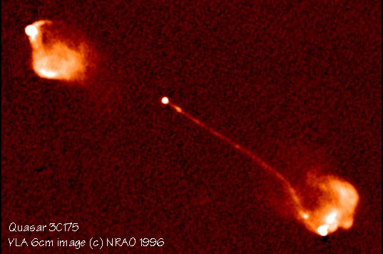
Figure 1: A gorgeous VLA map of a radio loud quasar, showing the parsec-scale core, the (apparently) one-sided jet, and the double lobes. Credit: National Radio Astronomy Observatory.

Linear features called jets connect the tiny (parsec-scale) radio cores to the lobes, feeding them energy in the form of relativistic electrons and magnetic field. But the jets often appear one sided! How is the other lobe energized…?

Certain radio loud quasars showed only point sources on early maps with $\sim 1$ arcsec resolution. These tiny (pc-scale, milliarcsec on the sky) radio cores could however be mapped with Very Long Baseline Interferometry, and they almost always turned out to show an even tinier (sub-pc) stationary point source, with a line of little blobs flying outwards along one side like cannonballs. This tiny linear feature is just the base of the larger-scale ($\sim 10$–100kpc) jet. The blobs appear to move perpendicular to the line of sight, often at about ten times light speed (this is called superluminal motion)! That would be very, very verboten in relativity. We also now know that quasar nuclei are at the centers of galaxies, primarily nascent galaxies in the early universe.

I wish to recount the history of quasars and the closely related objects called Active Galactic Nuclei (AGN), in such a way as to bring in the key observations and physical ideas. The term AGN has historically been used for 1) Seyfert galaxies (1940s) — which turn out to be just weaker versions of the “radio quiet” quasars. 2) radio galaxies, discovered in the 1950s. Many are just the lower-luminosity versions of radio-loud quasars. Today the quasars themselves are often grouped under the AGN rubric.

When the giant radio galaxies were discovered, two inferences were quickly made. One is that the Steady State theory of the universe (eternal, unchanging) was no longer tenable, because we observe a large excess of sources at faint flux levels relative to extrapolations from the bright sources. Roughly speaking, this requires that as we look far back in time towards the Big Bang, their space density increases, and thus the universe evolves!

The second inference is that the energy content of the radio lobes is astonishingly high. Suppose we want to make a very luminous synchrotron source, using as little energy as possible. (Suppose god is cheap.) To do this, we would put (approximately) equal amounts of energy into relativistic electrons and into magnetic field. So this case provides a lower limit to the amount of energy contained in the lobes, given their observed luminosity. The results are up to $1\times 10^{54-55}$ J, which by the equation $E=mc^{2}$ is the mass equivalent of about ten million stars like the sun! That is, one would have to (hypothetically) annihilate millions of stars and anti-stars to produce such energies. Where did this energy come from?

Some smart theorists, most notably D. Lynden-Bell in 1969, proposed that the energy production must involve gravitational collapse of hugely massive gas clouds ($1\times 10^{6}$–$1\times 10^{9}$ solar masses) to relativistic (near black-hole sized) dimensions. The energy available from gravitational collapse is extremely sensitive to the compactness of the final mass distribution. Collapse to relativistic dimensions results in almost a zero-divide in the potential energy released — enough to power the quasars. (This effect accounts for most of the “fireworks” throughout astronomy.) Furthermore the required black holes themselves would be only solar-system sized, consistent with the extremely small size upper limits based on rapid optical/UV variability, together with causality. That is, they are about one billionth the size of a galaxy.

I will only discuss the relativistic regions of AGN in this essay.

II What are the main observations and theories required to confirm and physically understand this scenario?

Here is my personal and very incomplete list.

• Do we see the required remnant (starved) black holes in the centers of nearby (present-day) galaxies, left over from the prime quasar era when the universe was $\sim 20$% of its present age?

• How, specifically, is the prodigious electromagnetic luminosity produced by gravitational collapse or infall?

• We find that very powerful radio (and optical, and X-ray) synchrotron-emitting plasma jets emerge from the central sub-parsec cores of some of them — but mysteriously, just the ones which reside in elliptical galaxy hosts! Why is that? Why should an engine of solar-system size care what type of galaxy it resides in?

• Why do these cores shoot “cannonballs” of plasma, often at apparently superluminal speeds, and apparently on only one side of the cores? The plasma jets feed the giant and extraordinarily energy-rich radio lobes. How does the bulk kinetic energy of the jet plasma get thermalized to produce the relaxed-looking giant lobes?

• How can we probe spacetime close to the putative black hole — can we prove that the Schwarzschild or Kerr solutions of Einstein’s equation for the spacetime geometry around a black hole are correct?

• We are only now becoming aware of the ecological role of the quasars’ immense radiative and mechanical luminosity in the formation of galaxies and stars. The probable importance of this AGN “feedback” became undeniable in the last 20 years when close connections were shown between the central black hole masses and the stellar content and internal (stellar) orbital velocities. And as noted, only those black holes that live in Elliptical (not Spiral) galaxies have the blockbuster radio power. Host galaxies won’t be discussed further in this article — but as a teaser, the quasar momentum and energy input may block further mass accretion onto a protogalaxy, and may in fact blow the interstellar gas out of the galaxy body, quenching star formation, and setting the maximum mass of (ordinary, “baryonic”) matter for these universal building blocks.

Only some of these great mysteries can be elaborated below.

III The “breakthroughs,” robust, dubious, and falsified

I will now enumerate the observations and interpretations that seem to most of the community to be the pillars of our understanding of AGN physics. In my opinion, several of these inferences are robust, others are dubious, and still others have been fully falsified, yet continue to be used by many researchers who seem to lack a good critical faculty, and who thus waste vast amounts of time and resources.

Many theory papers have already been ruled out by observations by the time they are published. Observers routinely use models to interpret their data long after the models have been falsified.

III.1 Prediction of Leftover Supermassive Black Holes: Robust Confirmation, 1980s-1990s.

An essential prediction of any gravitational collapse model is that leftover (starved) supermassive black holes (or other tiny objects) reside at the centers of most normal galaxies in the present universe, and this has been spectacularly verified, e.g. Kormendy 1988.

III.2 The Unified Model, Part 1: Relativistic beaming: Robust Confirmation, 1980s

Up until about 1980 or so, AGN were divided into many puzzling phenomenological subtypes based on correlated suites of observed traits. Much of the confusion was cleared up in the following decade: it turns out that while we see dramatically varied behavior, most of the differences depend only on the inclination of these roughly axisymmetric sources to the line of sight to Earth!

Figure 2: Illustration of the central parsecs of AGN. Shown are the Supermassive Black Hole, the accretion flow believed to be feeding the black hole and producing thermal optical/UV emission, the obscuring torus, and the jets, which are only strong in radio loud objects. The “torus” extends to the sublimation radius and its obscuration is primarily equitorial, but no implication is made regarding its actual shape and outer extent. (From Antonucci Nature 495, 165A, 2013)

This isn’t so surprising in retrospect: people have many systematic differences in appearance, depending on whether they are seen from the front or from the top. (The effect is relatively unimportant for stars because they are round.)

The superluminal speeds are now robustly attributed to motions actually at nearly light speed, traveling roughly (but not exactly) towards us along our line of sight. This is a classical effect due to sequentially lower light travel times for the little cannonball components shooting out of the radio cores as they move closer to us, producing the appearance of faster than light motions perpendicular to the line of sight. These sources are picked up preferentially because of the beaming (“headlight”) effect that comes from Special Relativity. In fact, this beaming effect nicely explains the apparently one-sided jets: we are quite sure now that there do exist “counterjets” so that both lobes are being energized, but the jet on the far side beams its radiation away from the line of sight! For a detailed observational review, see Antonucci 1993.

A spectacular corollary of the beaming idea is that there must be a much larger number of equivalent radio sources whose jets are not pointed at Earth. We now know that in most cases the misdirected objects are none other than the normal giant double sources (radio galaxies and the majority of radio quasars), which do not show fast superluminal motion as seen from Earth. The most conclusive evidence for the latter statement is that deep radio images of superluminal sources show large scale diffuse and isotropically emitting radio components as well as the tiny beamed cores. We must be able to see this diffuse emission in the misdirected objects, and only normal doubles have the right properties. Credit goes mostly to Peter Scheuer, Roger Blandford, Martin Rees, and Mitchell Begelman on the theoretical side. If you are a specialist and you think that a lot of progress has been made in AGN radio astronomy in the last thirty years though, you’d find it interesting to consult the long review by Begelman Blandford and Rees from 1984. The open questions of jet launching, acceleration, confinement, composition, equipartition, proton energies, and filling factors are still basically with us.

III.3 The Unified Model, Part 2: Hidden Nuclei: Discovery and Robust Confirmation, 1980s and 1990s.

Most optical spectra of both radio loud and radio quiet AGN come in two types (called Type 1 and Type 2!). The Type 2 sources have apparently simpler spectra, showing just a weak nuclear continuum which is constant in time, and often spatially resolved, plus a set of emission line clouds (the “Narrow Line Region”) with velocity widths of a few hundred km/s, and with densities more in the range of $1\times 10^{3}$–$1\times 10^{5}$ H atoms per cubic cm. These lines differ from those of H II regions in that they show much stronger high ionization lines, and also stronger very low ionization lines, compared with those of intermediate ionization. The difference is due to the extremely broadband exciting continuua in AGN relative to the stars that power H II regions.

Type 1 AGN show the exact same NLR, but much more. One also sees a strong unresolved and variable central source, including the energetically dominant “thermal” radiation component, or Big Blue Bump, in the optical/UV region, and also a collection of ionized gas clouds (the “Broad Line Region”) with collective Doppler-broadened line profile widths of a few thousand km/s. Certain line ratios prove that these clouds are relatively dense, $\sim 1\times 10^{10}$ H atoms per cubic cm. The Type 2 sources were thought to lack these essential nuclear components, and thus to differ fundamentally from the Type 1s.

My former thesis adviser Joseph Miller and I were able to sort this out by separating out a trace of polarized (reflected — as off your car windshield) light in the Type 2s from the much stronger direct light from stellar and gas emission. We used a natural gaseous and sometimes dusty “periscope” to see the hidden central regions of the Type 2 AGN “from above.” To our astonishment and delight, they look exactly like the ordinary directly visible Type 1 nuclei. The Type 2s must then just be unfavorably oriented from Earth’s point of view in that obscuring clouds of dusty gas lie in the line of sight. The scattering polarization position angle requires the obscuring material preventing our direct view (as opposed to the scattering polar “mirror” gas) to form (crudely) opaque tori of dusty gas whose axes are parallel to the radio structures, when the latter are detected. There is a very important caveat to all this: while the most luminous radio galaxies are all almost certainly quasars hidden by dusty tori, at lower levels of radio luminosity, many objects intrinsically lack the characteristic powerful optical/UV “thermal” continuum. Many arguments from observations at all wavelengths are reviewed in detail in Antonucci 2012. Also claims for the existence of “True Seyferts 2s,” said to behave like Type 1 objects except that they lack broad line regions intrinsically, are critiqued in detail in Section 2 of that paper. Most are found wanting.

III.4 The putative quasi-static accretion disk of inflowing matter. Falsified, 1980s–present.

Here we are discussing the “thermal” AGN such as quasars (Antonucci 2012), in particular the optical/UV Big Blue Bump component of their spectral energy distribution. This component is energetically dominant and nearly universally interpreted as optically thick thermal radiation which arises in the region of steeply falling potential region near the black hole.

“Wouldn’t It Be Loverly” (from My Fair Lady) if…as accreting matter spirals down the gravitational potential well, it radiates the incrementally released gravitational potential energy right where it’s produced? (I’m ignoring a couple of unimportant subtleties…) The region where (effectively) most of the potential drop occurs has a size of a few to $\sim 10$s of times the event horizon radius, which for a non-rotating black hole is given by the formula 3 km times the black hole mass in terms of the Sun’s mass. This idea, together with the key assumption of a “quasistatic” flow in which the inflow timescale is much larger than the other timescales in the problem — roughly but robustly — predicts a certain spectral energy distribution (amount of light at each frequency across the electromagnetic spectrum). Alas, this prediction was falsified almost immediately after the model was first used (Shields 1978, Malkan 1985). A key here was the realization that the infrared radiation is from hot dust, and it cannot be extrapolated under the optical spectrum to help with the fitting as was done in the early disk papers.

On the other end of the spectrum, the standard model predicts an exponential falloff from the Wien part of the quasi blackbody radiation from the innermost disk annulus, which is never seen, but can be hidden with plausible but ad hoc Comptonization.

There are two possible candidates for some type of spectral feature from the inner disk edge. Many sources show a puzzling break (slope steepening) below $\sim 1000$Å. Though not an exponential, this might conceivably be identified with an inner disk temperature. Unfortunately, according to the models, it can’t be fixed in wavelength as observed; it must depend on black hole mass, Eddington ratio, and spin. Similarly, there is a generic “Soft X-ray Excess” in thermal AGN such as quasars. It’s not clear whether this should be considered an extension of the Big Blue Bump, but it’s energy ($\sim 200$eV) is again the same for all objects, a fatal flaw for the standard disk model and almost all of its variants.

Falsifications of other robust predictions soon followed. In fact they were already implicitly falsified by existing data. For example, AGN are highly variable. The region in which the bulk of the radiation from a standard accretion disk arises is fixed over human timescales because it’s set by the black hole mass. Therefore it must show a temperature increase roughly in proportion to $L^{1/4}$ which is irreconcilable with the observations (e.g. Ruan et al 2014). This prediction is based on two extremely mild assumptions: the validity of the Stefan-Boltzmann Law (the luminosity per square meter of a blackbody radiator is proportional to temperature to the fourth power), and the size of the event horizon radius (and perhaps the innermost stable circular orbit) from general relativity. As a quasar continuum luminosity is seen to vary (necessarily in this scenario, it’s radiated from a fixed area), it follows that one should be able to fit a temperature for the inner edge of such an accretion disk, and it should vary according to T proportional to $L^{1/4}$. This behavior has been seen in the accretion disks inferred for black hole binaries! In most [but not all!] AGN, the continuum does become bluer, but the frequently seen slope change remains at the generic rest wavelength of 1000Å, as does the Soft X-ray Excess.

There have been a few critiques of these models over the years, including Antonucci et al 1989, 1999; Courvoisier and Clavel 1991; and Blaes 2007. Most theorists now acknowledge that the proposed workarounds are themselves seriously problematic.

These and other demurs were roundly and uncritically dismissed for decades (and currently!) by almost the entire community, and enormous effort has been spent refining this erroneous model. This is a powerful example of the wheel-spinning in our community which prevents us from making rapid progress.

The theoretically essential quasi-static assumption was falsified explicitly when it was shown that the optical continuum varies closely in phase with the hydrogen-ionizing continuum (photons with energies above 1 Rydberg); see Alloin et al 1985; Krolik et al 1991. But we already knew enough about quasar variability at that time to tell us we were on the wrong track.

Might the optical/UV emitted still be some kind of chaotic blackbody disk of indeterminate physics, but which somehow mimics the quasistatic disk morphologically? Even this hope has been falsified. Recently ($\sim 2000$’s) the angular size-measuring technique called gravitational microlensing has produced approximate but consistent and reliable source sizes for these heretofore emitting regions, and they are typically several times as large as they can possibly be in any standard disk models! (The sizes are quite approximate in individual cases, but the whole data set together is compelling.) That is, the surface brightness of the optical/UV radiator is only a few percent of that of a blackbody or any disk that fits the spectra slopes locally. This is incredibly important because it means the radiation doesn’t come from the region in which the energy is released. I conclude from this that we know next to nothing about the fundamental physics of radiation from AGN.

I can’t take a model seriously if it doesn’t produce a surface brightness of the right order of magnitude. Dexter and Agol (2011) presented a toy model for a disk which is mostly dark at any particular wavelength, but has bright (atypically hot) spots; that way the overall size of the source could be increased to match the observations. This seems promising because polarization data do indicate that optically thick emission makes the Big Blue Bump (Kishimoto et al 2004, 2008). Few if any other theorists have even tried to build the game-changing microlensing sizes into their models.

Recently two theory groups proposed that the standard model might apply in small regions of parameter space. According to one set of authors, the golden objects are those with low $M$, high Eddington ratio, and very high predicted temperature which could explain the Soft X-ray Excess (though that doesn’t seem very satisfying since that feature is generic). According to the other group of theorists, the best hope lies in objects in the opposite part of parameter space: extremely massive black holes with low Eddington ratios, and predicted very cool disks. Neither group claims the quasistatic model has relevance for the vast majority of objects.

Yet characteristic values and scaling relations based on the quasi-static disk model are still routinely used by most authors, generally without apology. Remember that the observations don’t just rule out quasi-static models (the only ones with predictive power!): the sizes rule out energy release following the gravitational potential well expected for all black holes. That means we aren’t even close to having the correct physics.

III.5 Secrets of the X-ray Spectrum: Mapping out the Kerr potential Dubious, 1990s–present

In 1995, because of the advancement in X-ray spectroscopy from space represented by the ASCA mission, it became possible to study the emission line profiles in the brightest Seyfert 1s.

The strongest spectral feature in thermal AGN is the Fe K$\alpha$ line, which has a rest-frame energy of 6.4 keV if it’s neutral, and up to 6.9 keV if it’s highly ionized. A discovery [with antecedents of course] was announced by Tanaka et al in 1995 that almost everyone (including me) thought was a breakthrough we were all waiting for. This line was reported to be neutral and very broad in MCG 6-30-15, of order 100,000 km/s, with a particularly extended red wing to the apparent profile assuming no “warm absorption.” A (very noisy) “horn” appeared on the red side of the profile, which would be suggestive of a disk origin.

Such profiles were interpreted as indicating the effects of Doppler shifts from very fast motions and gravitational redshifts of the gas. This suggests that they are produced very close to the putative supermassive black holes. In particular, it was argued that this line is produced by external illumination of relatively cool gas, arranged in an accretion disk, by a (mysterious but real) X-ray continuum source hovering above the putative disk. The far side is of course similar, but unseen.

To some extent in this scenario, we’d be mapping out the relativistic region of the putative supermassive black hole. This ultimate key region had never been explored so directly before.

The cleanest test of this disk-reprocessing interpretation in my opinion is to see whether the emission line luminosity responds in real time to changes in the driving continuum luminosity. It took almost no time for some of the same authors as those of the Fe K$\alpha$ discovery paper, using the same exact 4 day long data set, to falsify the prediction (Iwasawa et al 1996), although with much special pleading they claimed they could save the model. Iwasawa et al showed that the published “disk-like” [e.g. the noisy red horn] spectrum averaged over the 4 day integration never actually existed at any one time! It was an artifact of the summing over the particular observing interval, which was set not for a physical motivation but by scheduling and competition from other proposals.

For many years before and after the discovery, all authors similarly reported that the lines do not respond intelligibly to continuum changes on short (light travel) timescales, as virtually required by the models. Only a very few critical thinkers seemed to care about this cognitive dissonance.

Minuitti et al (2003) did care about the problem, and developed what I consider to be an epicycle, called the “light bending model.” (It’s called a model though it has very little physics in it.) The model asserts that the hovering X-ray continuum (called the corona) comes not from a fixed height above the putative disk, the previous fiducial scenario adopted to minimize free parameters. Instead the corona can now be raised and lowered as needed to fit the data. In particular, the ubiquitous rapid continuum variability in thermal AGN was seen as illusory, a result of rapid vertical motions of the “corona,” which would throw a highly variable flux our way, but conspire to deliver a relatively constant driving luminosity to the K$\alpha$ emitter. Again, the sole purpose was to explain (away) the lack of line response by attributing the continuum changes not to actual changes in power. But the lines do vary, they just don’t follow the continuum. Nevertheless sufficiently violent and ad hoc vertical motions of the corona could scramble the correlation between the driving continuum and the K$\alpha$ line, and to scramble it so much that it can never be recognized. This paper made some predictions…I’m not aware of any claims that they came true, but to my surprise, most of the community seemed to be satisfied that these authors “solved” the problem. All you have to do is say, “Light bending!”

Incidentally, the X-ray illumination must also move around above the disk in the radial and azimuthal directions in an ad hoc manner to produce the changing bumps and wiggles in the observed profile (Iwasawa et al 1996).

Cooler heads such as T J Turner, K Weaver, T Yaqoob, L Miller and several others have produced plausible (if less exciting) explanations for the apparent far red wings of the X-ray Fe K$\alpha$ line profile as largely a spurious interpretation of the effects of absorption from ionized gas in front of the continuum sources. Complex and variable ionized and neutral absorbing matter is almost ubiquitous in AGN, and well documented. Miller et al (2009) showed that even the discovery object, MGC 6-30-15, can be very well fit this way, and it resolves the problem of the lack of intelligible line response to an apparently changing continuum.

The highly ionized absorbing gas (the “Warm Absorbers”) are well studied and very widespread. When one concentrates on the few “clean” objects which happen to have weak absorption (clearly the best thing to do), the crucial far red wings no longer appear! Some great examples were shown by Patrick et al in 2011, who demonstrated that only modestly broadened lines are allowed by the data (and not necessarily even needed). Interestingly, the original poster-child, MGC 6-30-15, is very “dirty” in the sense that it has strong, variable, and complex absorption, and as noted, can be modeled with no broad K$\alpha$ line at all (Miller et al 2009).

Now let’s go back to the contentious issue of the response of the fluorescence line to continuum changes. Many of the same authors that found no line response to continuum changes previously have changed their analysis method and now find that the lines do show this effect!

In the optical regime, the study of the response of the broad emission lines to continuum changes is extremely well developed. The standard and minimum acceptable demonstration of line response requires: 1) a clearly shown line/continuum separation. This is much more important, but largely lacking, in the X-ray papers. They very rarely show figures which allow the reader to form an opinion on the decomposition, and it’s so important because of the claimed extreme breadth of the line. 2) light curves for the continuum and line flux; 3) a cross-correlation curve showing the line flux response over time. It can be made for separate parts of the profile if the signal to noise ratio is high.

X-ray astronomers claiming line responses to continuum changes never (as far as I know) follow any of these precepts. These failings interact in a pernicious way. For example, there are well documented complex interband continuum phase lags in AGN X-ray spectra, so that even if a phase lag is correctly inferred in the region of the putative far red K$\alpha$ wing relative to the Fe-ionizing continuum, it might arise from the underlying continuum. As examples, Legg et al (2012) and Miller et al (2010) should be consulted.

The reason some astronomers find line responses today is that they have adopted a new method with a lot more freedom and subjectivity. These authors now take only particular Fourier components of the line and continuum light curves, and find some lags by selecting the Fourier frequencies a posteriori. Time will tell if the newly reported short lags are real.

Also the papers that that I know which report time lags look for phase differences between the line and continuum at the same temporal frequency. But the response should actually be smoothed out by light travel time across the reprocessor, so as I understand it, the analyses aren’t self-consistent. I think it would be far more reliable to calculate the cross-correlation and just display the response (“Transfer”) function. This could be done as a function of energy within the profile, as optical astronomers do.

These papers may all be correct but disk fluorescence proponents seem to invoke more and more epicycles as the monitoring data improve. If the lags inferred for the different parts of the line profile are set by the geometry of a spinning quasi-Keplerian disk, shouldn’t they stay about the same over time? Please read Alston et al. 2013, Sec. 4, as an example of what can really happen. Another example is discussed by Kara et al (2014). It’s also worth noting that extravagant abundances are sometimes required, e.g. 7–20x solar M1H0707-493; see discussion in Done and Jin (2015).

Switching gears slightly, the very small radius of the innermost stable circular orbit for rapidly rotating black holes has led to a substantial literature running the argument backwards: a highly redshifted wing, for which the observed line energy is only $\mathrel{\raise 1.29167pt\hbox{$<$\kern-7.5pt\lower 4.30554pt\hbox{$\sim$}}}$ half the rest energy, requires a rapidly spinning hole. So there are many fits to line profiles which people use to infer black hole spin. In fact this is now a huge and widely accepted industry. To get an idea of the robustness of spins inferred from X-ray spectra, please read Sec. 4.3.4 from Patrick et al. (2012) on the spin of the Seyfert NGC 3783. In the previous paper (Patrick et al 2011) of this outstanding series of three, the authors analyzed a magnificent 210 ksec Suzaku observation, placing an upper bound of 0.31 on the spin parameter. The exact same data were analyzed in Brenneman et al (2011); those authors could say with 90% confidence that the value is greater than 0.98.

The situation seems little better for X-ray binaries. For example, recent papers on Cyg X-1 have reported values of $0.05\pm 0.01$ and $0.97\pm 0.014/-0.02$, where even the asymmetry of the tiny errors has been quantified.

Another puzzle in the disk interpretation: they are undetected at a constraining level in most AGN, yet are attributed to the essential relativistic accretion process thought to provide all of the energy to thermal AGN generically.

Now let’s try to combine the “great discoveries” of the optical/UV emitting accretion disk and the spin-measuring Fe K$\alpha$ profiles.

The (falsified) standard thermally emitting optical/UV-emitting accretion disk gets the bulk of its energy from basically the same relativistic region where the Fe line arises. Yet there is almost no known empirical connection between the emitting disks and the flourescing disks, which are considered as purely passive reprocessors in all X-ray modeling that I’ve seen. Yet close connections are expected. For example, most fluorescence models, and all those reporting spins, require that the disks extend as optically thick geometrically thin structures to only a few gravitational radii, in particular to the innermost stable circular orbit. The inner edges of such disks should be very hot, and this should be manifest as very blue UV/FUV continua, yet this is virtually never seen. In fact, observation-oriented theorists trying to fit optical/UV spectra to accretion disk models must truncate the disks well outside this region (e.g. Jin et al 2012; Done et al 2012; Laor and Davis 2014)!

Again, relatively few astronomers seem to be bothered by the cognitive dissonance.

IV A few observations and calculations which could address these problems fundamentally

IV.1 Advanced X-ray reverberation mapping

Really robust and detailed line/continuum response studies with future advanced X-ray telescopes will tell us a lot about what we really want to know: the spacetime geometry and mass flows in the innermost regions of the highly warped spacetime extremely close to the black holes.

IV.2 Getting the true central-engine optical/UV spatial energy distribution

We observers owe the theorists real spectral energy distributions of the energetically dominant “central engine” radiation, that is, without the daunting contributions from various kinds of reprocessed emission. In some regions of the optical/UV spectra, small nearly-pure continuum windows are available, but in large wavelength intervals this is not the case. Yet it is possible to measure the true continuum emission in some cases using polarimetry. Small but very successful beginnings at discovering the true shape and spectral features of the Big Blue Bump have been published by Kishimoto et al 2004, 2008 and references therein. We have found that in certain quasars, the optical continuum comes to us with a small but detectable electron-scattered fraction, and it is thus slightly polarized; this is physically similar to the periscope affect discussed above in the context of Unified Models, but on scales of order a million time smaller. It’s a fantastic piece of luck because the contaminating components (starlight from the host galaxy, atomic emission lines and bound-free continua, and infrared radiation from glowing solid particles) are sometimes all unpolarized. So we need only plot the polarized flux spectrum to see the isolated central engine spectrum! We’ve discovered the first spectral feature intrinsic to the actual AGN engines in this way, absorption in the Balmer continuum (Kishimoto et al 2004). We also know that there is a sharp slope change longward of $1\mu$ (Kishimoto et al 2008): the central engine spectra are much bluer in the near-IR than in the optical, with spectral index $\sim+0.3$, when the dust emission is removed with polarimetry. Later several objects were found with intrinsically weak near-IR dust emission, and this blue slope was confirmed in total flux.

IV.3 Advanced numerical simulations

Very detailed relativistic magnetohydrodynamic simulations of matter flowing into a black hole, with the inclusion of such essentials as dissipation and radiation will be required. Software breakthroughs, aided by Moore’s law, are starting to achieve some traction in certain special cases. So far we have only explored this method down to around 3000Å in the rest frames, at high SNR, but we have taken data pushing down through and past the Small Blue Bump covering 2000-4000Å to find the shape in this heavily contaminated region, and we are also exploring the Ly continuum region where very surprising but tentative results have been reported. It goes without saying that this is incredibly difficult.

IV.4 The Green’s Functions for AGN: Tidal Disruption Events

One thing we know about AGN is that they are a complicated mess. Theorists need a simple well-defined problem with known initial conditions. After M Rees whipped us into a frenzy of excitement about it in 1988, many of us have waited for the day when we could observe isolated starved black holes, and then throw a single simple piece of matter (a star!) into them, sit back and see what happens! I call the various resultant displays the “Green’s Functions” for supermassive black hole accretion. Such events have been persuasively identified by S Komossa and others — the data gathered during the events so far is limited, but this is improving rapidly. Will we see short-lived quasars when this happens? Feast your eyes on recent papers such as Yang et al 2013 and Arcavi et al 2014. This is the most exciting thing going on in the AGN field today.

References

Appendix: Some poor practices in AGN research

For those with a taste for spleen, I present a list of some practices which are almost generic in AGN research, but which seem erroneous to me. This is an idiosyncratic list, written using the stream-of-consciousness technique. Please let me know where I’ve gone wrong.

1. Vast amounts of observing time have been spent on spectra of AGN and infrared galaxies, at telescopes with polarimetry modules that the observers didn’t both to place in the beam. Yet look at the value this often adds. For example, observers wasted a lot of Keck time taking spectra of Cygnus A in search of weak broad emission lines. None were detected, and tight (but spurious) upper limits were claimed. Please look at Ogle et al 1997, Figs. 1 and 2, which resolved the situation entirely. Similarly thousands of quasar spectra have been taken in total flux, though polarization could have been taken almost for free. As noted earlier, Kishimoto et al (2008) used the polarized flux of some clean objects to get to the intrinsic spectrum of the central engine. A huge amount of work has been done on the host galaxies of Type 1 quasars in total flux mode, with crippling contamination by nuclear light. This is despite the fact that we know (e.g. from spectropolarimetry) that Type 2 quasars are the same objects, but with Nature’s coronagraph completely blocking the nuclear light.

Infrared galaxies often have spectacular polarization properties. Take a look at G. Schmidt (1975)’s image of M82, achieved with a 2.4m telescope, photographic plates (!!), and 12 minutes of exposure time per waveplate position. The extremely high polarization of the lines as well as the continuum ($\sim 25$%) means that much of the emission is not produced in situ, but it has been analyzed as if it were. One could also observe high latitude clouds to find the spectrum of M82 “as seen from above.” The dust can also provide an approximate but robust estimate for the cool-phase mass, a key ingredient in galactic wind models. We (Hoenig et al) have gathered some great polarization images of other infrared galaxies. At the high luminosity end, all of the original “Hyperluminous” infrared galaxies show quasars in polarized flux. It’s too bad people spent all that time on total flux spectroscopy. Of course a high-ionization infrared galaxy is just another name for a luminous Type 2 AGN.

In order to get the polarization at Keck, you have to type “POLAR $<$cr$>$.” There are no plans for polarization analyzers on any of the big new telescopes being built, because no one uses the instruments on the current telescopes.

2. Plots of one luminosity measure vs. another within a class of objects almost always find good correlations, because big things are bigger. Consider a plot of the number of bookstores vs. the number of bars in cities and towns across America. I’d expect a great correlation over many orders of magnitude, with perhaps modest dispersion and essentially infinite statistical significance. Everyone knows that doesn’t mean that readers like to drink, or that drinkers like to read. I’m tempted to give an example of a very influential paper from 1991 which used this method to arrive at an erroneous conclusion that took a decade or two to fuzzily reverse. The key reference illustration here is Kennicutt (1996), where he shows a plot of CO vs. far-IR luminosity for galaxies, but then to extend the baseline he adds a burning cigar, a Jeep Cherokee Wagon, the 1988 Yellowstone park forest fire, Venus, and the observable universe.

It’s helpful to plot the fluxes as well as the luminosities. Flux plots are also dangerous, but the horrible biases introduced are different from those with luminosity, so when the correlation shows up in both, I get a warm feeling. Note that I am by no means an expert in statistics.

3. Another extremely common type of plot involves A vs. B/A or some other mathematically dependent or partially dependent quantities. The dependence is often hidden because one or both observables are relabeled as physical quantities based on some dodgy model. Of course if A and B are unrelated, you are guaranteed a spurious negative correlation, if there is a finite amount of intrinsic dispersion or observational error. The significance will be arbitrarily high if you have a lot of objects. Egg-shaped distributions are especially suspect. Even if a “real” correlation is present, the bias contributes to the apparent correlation, so that the slope isn’t meaningful in general, yet such slopes are routinely quoted and used.

There are some plots, I think those with narrow low-dispersion features and only very mild dependences of the axes, for which this bias isn’t important. An example is the HR Diagram. But diagrams of $B-V$ vs. $V$ should really use some kind of average of $B$ and $V$ for the dependent variable.

4. The Gaussian function is extremely pathological because the far wings are vanishingly small. (Think of the Curve of Growth.) The distribution involves the exponential of the square of a deviation from an apparent correlation line. Since outliers are impossibly unlikely, in such a distribution, you can rule out a null result with one object. Few quantities used by astronomers are Gaussian-distributed. It works for thermal noise, counting photons, etc, but for few if any actual population distributions of macroscopic objects.

5. How do astronomers treat limits in null and correlation tests? To use limits “correctly”, a survival function must be invoked and rationalized. Astronomers arbitrarily pick something like Proportional Hazards (e.g. the Kaplan-Meier method) without any basis, or even comment. These approaches, derived in the context of actuarial tables, have no obvious applicability to astronomical data sets, which depend on luminosity, flux, or other distributions which are a priori unknown.

6. As noted, many X-ray astronomers in particular decline to plot fully calibrated data covering the entire observed energy range. Instead they show count spectra, spectra without enough coverage of the “continuum” to judge the believability of the Fe K-$\alpha$ far wings, or most appallingly, spectra divided by models! I’d like to see an optical paper showing only spectra divided by Cloudy models. These authors are to some extent selling models, and the process reminds me of an actual Freudian slip: “I’ll see it when I believe it.”

7. It’s still extremely common for people to mis-state the meaning of null test statistics. For example, “The thick lines indicate where a Welch’s $t$ test shows the mean SEDs have less than a 1% chance of being the same ($p<0.01$).” (I read this aloud to a particle physicist analyzing LHC data because he happened to be in my office and he burst out laughing.)

No, the test shows that uncorrelated data would, in a certain sense, look as correlated as yours (in your chosen test statistic) only 1% of the time. This is certainly not a semantic issue. In my critical thinking lesson for the Astro 1 Honors section, I show a stupid (old) article from a financial magazine which noted that over the previous 10 years, two methods of predicting the next year’s stock market performance worked equally well, getting the correct result 9 times. One involved insider trading: lots of buys portend a rising market. The other method was based on whether an American Football League or a National Football League team won the championship. The statistical significance is the same. Then I ask which method they would use for investing their retirement account funds and they get it right away.

Steve Reynolds once told me the First Theorem of Metastatistics: “Half of all 3-sigma results are true.” (He’s since raised it to 5-sigma.) And here is an apocryphal quotation attributed to Martin Rees: “It would be really funny if nothing funny ever happened.”

8. In comparing samples to see whether or not they may differ only in orientation, a mighty torrent of negative results were reported for many years, both in the context of the beam model, and then all over again for the torus model. It was pointed out that e.g. the Seyfert 1 prototype, NGC 4151, has much weaker emission in the IR, in CO, etc, compared with the Seyfert 2 prototype NGC1068. Therefore they can’t differ only in orientation. Only trouble is, if we select by something like UV excess, which is comparable in the two objects, we are comparing the actual luminosity of NGC 4151, to the 1% of the luminosity which is scattered into the line of sight for NGC 1068. So NGC 1068 is 5 magnitudes higher on the luminosity function. No wonder it has more of everything. In the history of testing the beam model, properties of superluminal sources were compared with those of big luminous FR II doubles; since the former were selected on the beamed emission, they turned out to have much lower diffuse lobe emission, way down in the FR I range in most cases. You must select your sample on some hopefully nearly isotropic property of the AGN. It does not work to select on the host galaxies.

9. What is the AGN torus? Joe Miller and I didn’t introduce that term, and didn’t draw an outer boundary for the equatorial obscurer, because we had no information on that. The torus is historically defined to be the thing that causes optical nuclear photons to escape preferentially in the polar direction, the polarization position angle having been found to be perpendicular to the radio axes in Type 2 objects. The anisotropy is very substantial because the percent polarization of the scattered light is usually relatively high (at least by selection). Unspecified is the radius at which the shadowing occurs, except that it must be inside the narrow line region. But it’s likely that they are quite messy: see what I call the (very) “Sloppy Torus” CO source in NGC 1068, Garcia-Burillo et al 2014; it looks most torus-like in Fig. 4. The dynamics are already known to be complex. In some cases the torus may just be a dusty wind. The fast growing field of infrared interferometry will tell us a lot, as will the very sensitive and sharp ALMA millimeter array.

One should never refer to the size of the torus without stating exactly what you mean for this edge-darkened source. It does seem clear though that essentially every thermal AGN has a significant covering factor of dust at the sublimation radius, so the inner boundary is relatively well constrained.

10. There is an industry finding, studying and theorizing about objects which are like Seyfert 1 nuclei, but “lack broad lines.” I urge anyone interested in this literature are urged to read my critical comments in Sec. 2 of Antonucci 2012. Few of the preferred candidates are strong. I’ll take this last chance to tout that long detailed review of unification and central engine types, which carefully covers the data at all wavelengths.

11. The mainframe (!) computer went down one day when I was a young postdoc at STScI. All the astronomers were huddled in the library, reading papers and discussing science instead of pecking away at their terminals. Visiting Santa Cruz, California, I saw a bumper sticker with the wisdom of that fair city: “Don’t just do something, sit there.”

12. A great many papers refer to the peak of a spectrum and the corresponding temperature for a blackbody emitter. But there is no consistency on how the peak is defined. In fact it’s not usually even specified.

The solar spectrum is said to peak at a wavelength of $5\times 10^{-7}$m, which comes from Wien’s blackbody law, $\lambda_{\rm max}=2.9\times 10^{-3}$ m $K/T$. This applies only to a plot of flux (or intensity) per unit wavelength interval, $F_{\lambda}$, and makes objects seem “bluer” than they really are. This is easy to see: many astrophysical objects emit strongly in the x-ray and gamma ray. In a plot of flux per nanometer, for example, the entire hard X-ray and gamma ray luminosity would fall into a single bin, the one going from 0 nm to 1 nm! Plots of the flux per unit frequency are similarly flawed, but in the opposite sense.

When plotting a wide band spectral energy distribution, almost all astronomers now use $\nu F_{\nu}$ or, equivalently, $\lambda F_{\lambda}$. This is proportional to flux per unit logarithmic frequency or wavelength interval, or more simply, flux per decade. This shows the actual distribution of flux across the spectral energy distribution. The equivalent of Wien’s law when plotting $F\nu$ is approximately $\lambda_{\rm max}=5.1\times 10^{-3}\ {\rm mK/T}$, which corresponds to an apparent spectral peak of $\nu_{\rm max}=(5.9\times 10^{10}\ {\rm Hz/K)T}$. When plotting the recommended $\nu F_{\nu}$, the peak $\lambda_{\rm max}$ occurs at $3.7\times 10^{-3}\ {\rm mK/T}$ and $\nu_{\rm max}=8.2\times 10^{10}\ {\rm T(Hz/K)}$.

References

- Alloin et al. 1985 D. Alloin, D. Pelat, M. Phillips, and M. Whittle, Astrophys. J. 288, 205 (1985).
- Alston et al. 2013 W. N. Alston, S. Vaughan, and P. Uttley, MNRAS 435, 1511 (2013), arXiv:1307.6371 [astro-ph.HE].
- Antonucci et al. 1989 R. R. J. Antonucci, A. L. Kinney, and H. C. Ford, Astrophys. J. 342, 64 (1989).
- Antonucci 1993 R. Antonucci, ARA&A 31, 473 (1993).
- Antonucci 1999 R. Antonucci, in High Energy Processes in Accreting Black Holes, Astronomical Society of the Pacific Conference Series, Vol. 161, edited by J. Poutanen and R. Svensson (1999) p. 193, astro-ph/9810067.
- Antonucci 2012 R. Antonucci, Astronomical and Astrophysical Transactions 27, 557 (2012), arXiv:1210.2716 [astro-ph.CO].
- Antonucci 2013 R. Antonucci, Nature (London) 495, 165 (2013).
- Arcavi et al. 2014 I. Arcavi, A. Gal-Yam, M. Sullivan, Y.-C. Pan, S. B. Cenko, A. Horesh, E. O. Ofek, A. De Cia, L. Yan, C.-W. Yang, D. A. Howell, D. Tal, S. R. Kulkarni, S. P. Tendulkar, S. Tang, D. Xu, A. Sternberg, J. G. Cohen, J. S. Bloom, P. E. Nugent, M. M. Kasliwal, D. A. Perley, R. M. Quimby, A. A. Miller, C. A. Theissen, and R. R. Laher, Astrophys. J. 793, 38 (2014), arXiv:1405.1415 [astro-ph.HE].
- Begelman et al. 1984 M. C. Begelman, R. D. Blandford, and M. J. Rees, Reviews of Modern Physics 56, 255 (1984).
- Blaes 2007 O. Blaes, in The Central Engine of Active Galactic Nuclei, Astronomical Society of the Pacific Conference Series, Vol. 373, edited by L. C. Ho and J.-W. Wang (2007) p. 75, astro-ph/0703589.
- Brenneman et al. 2011 L. W. Brenneman, C. S. Reynolds, M. A. Nowak, R. C. Reis, M. Trippe, A. C. Fabian, K. Iwasawa, J. C. Lee, J. M. Miller, R. F. Mushotzky, K. Nandra, and M. Volonteri, Astrophys. J. 736, 103 (2011), arXiv:1104.1172 [astro-ph.HE].
- Courvoisier and Clavel 1991 T. J.-L. Courvoisier and J. Clavel, A&A 248, 389 (1991).
- Done et al. 2012 C. Done, S. W. Davis, C. Jin, O. Blaes, and M. Ward, MNRAS 420, 1848 (2012), arXiv:1107.5429 [astro-ph.HE].
- Done and Jin 2015 C. Done and C. Jin, ArXiv e-prints (2015), arXiv:1506.04547 [astro-ph.HE].
- Edelson et al. 2015 R. Edelson, J. M. Gelbord, K. Horne, I. M. McHardy, B. M. Peterson, P. Arévalo, A. A. Breeveld, G. De Rosa, P. A. Evans, M. R. Goad, G. A. Kriss, W. N. Brandt, N. Gehrels, D. Grupe, J. A. Kennea, C. S. Kochanek, J. A. Nousek, I. Papadakis, M. Siegel, D. Starkey, P. Uttley, S. Vaughan, S. Young, A. J. Barth, M. C. Bentz, B. J. Brewer, D. M. Crenshaw, E. Dalla Bontà, A. De Lorenzo-Cáceres, K. D. Denney, M. Dietrich, J. Ely, M. M. Fausnaugh, C. J. Grier, P. B. Hall, J. Kaastra, B. C. Kelly, K. T. Korista, P. Lira, S. Mathur, H. Netzer, A. Pancoast, L. Pei, R. W. Pogge, J. S. Schimoia, T. Treu, M. Vestergaard, C. Villforth, H. Yan, and Y. Zu, Astrophys. J. 806, 129 (2015), arXiv:1501.05951.
- García-Burillo et al. 2014 S. García-Burillo, F. Combes, A. Usero, S. Aalto, M. Krips, S. Viti, A. Alonso-Herrero, L. K. Hunt, E. Schinnerer, A. J. Baker, F. Boone, V. Casasola, L. Colina, F. Costagliola, A. Eckart, A. Fuente, C. Henkel, A. Labiano, S. Martín, I. Márquez, S. Muller, P. Planesas, C. Ramos Almeida, M. Spaans, L. J. Tacconi, and P. P. van der Werf, A&A 567, A125 (2014), arXiv:1405.7706.
- Iwasawa et al. 1996 K. Iwasawa, A. C. Fabian, C. S. Reynolds, K. Nandra, C. Otani, H. Inoue, K. Hayashida, W. N. Brandt, T. Dotani, H. Kunieda, M. Matsuoka, and Y. Tanaka, MNRAS 282, 1038 (1996), astro-ph/9606103.
- Kara et al. 2014 E. Kara, A. C. Fabian, A. Marinucci, G. Matt, M. L. Parker, W. Alston, L. W. Brenneman, E. M. Cackett, and G. Miniutti, MNRAS 445, 56 (2014), arXiv:1408.5051 [astro-ph.HE].
- Kennicutt 1997 R. C. Kennicutt, in Astrophysics and Space Science Library, Astrophysics and Space Science Library, Vol. 161 (1997) pp. 171–195.
- Kishimoto et al. 2008 M. Kishimoto, R. Antonucci, O. Blaes, A. Lawrence, C. Boisson, M. Albrecht, and C. Leipski, Nature (London) 454, 492 (2008), arXiv:0807.3703.
- Kormendy 1988 J. Kormendy, Astrophys. J. 325, 128 (1988).
- Krolik et al. 1991 J. H. Krolik, K. Horne, T. R. Kallman, M. A. Malkan, R. A. Edelson, and G. A. Kriss, Astrophys. J. 371, 541 (1991).
- Legg et al. 2012 E. Legg, L. Miller, T. J. Turner, M. Giustini, J. N. Reeves, and S. B. Kraemer, Astrophys. J. 760, 73 (2012), arXiv:1210.0469 [astro-ph.HE].
- Lynden-Bell 1969 D. Lynden-Bell, Nature (London) 223, 690 (1969).
- Malkan 1983 M. A. Malkan, Astrophys. J. 268, 582 (1983).
- McHardy et al. 2014 I. M. McHardy, D. T. Cameron, T. Dwelly, S. Connolly, P. Lira, D. Emmanoulopoulos, J. Gelbord, E. Breedt, P. Arevalo, and P. Uttley, MNRAS 444, 1469 (2014), arXiv:1407.6361 [astro-ph.HE].
- Miller et al. 2010 L. Miller, T. J. Turner, J. N. Reeves, and V. Braito, MNRAS 408, 1928 (2010), arXiv:1006.5035 [astro-ph.HE].
- Ogle et al. 1997 P. M. Ogle, M. H. Cohen, J. S. Miller, H. D. Tran, R. A. E. Fosbury, and R. W. Goodrich, ApJ 482, L37 (1997), astro-ph/9703153.
- Patrick et al. 2011 A. R. Patrick, J. N. Reeves, A. P. Lobban, D. Porquet, and A. G. Markowitz, MNRAS 416, 2725 (2011), arXiv:1106.2135 [astro-ph.HE].
- Patrick et al. 2012 A. R. Patrick, J. N. Reeves, D. Porquet, A. G. Markowitz, V. Braito, and A. P. Lobban, MNRAS 426, 2522 (2012), arXiv:1208.1150 [astro-ph.HE].
- Rees 1988 M. J. Rees, Nature (London) 333, 523 (1988).
- Ruan et al. 2014 J. J. Ruan, S. F. Anderson, J. Dexter, and E. Agol, Astrophys. J. 783, 105 (2014), arXiv:1401.1211 [astro-ph.HE].
- Schmidt et al. 1976 G. D. Schmidt, J. R. P. Angel, and R. H. Cromwell, Astrophys. J. 206, 888 (1976).
- Shields 1978 G. A. Shields, Nature (London) 272, 706 (1978).
- Tanaka et al. 1995 Y. Tanaka, K. Nandra, A. C. Fabian, H. Inoue, C. Otani, T. Dotani, K. Hayashida, K. Iwasawa, T. Kii, H. Kunieda, F. Makino, and M. Matsuoka, Nature (London) 375, 659 (1995).
- Yang et al. 2013 C.-W. Yang, T.-G. Wang, G. Ferland, W. Yuan, H.-Y. Zhou, and P. Jiang, Astrophys. J. 774, 46 (2013), arXiv:1307.3313.
- Zakamska et al. 2005 N. L. Zakamska, G. D. Schmidt, P. S. Smith, M. A. Strauss, J. H. Krolik, P. B. Hall, G. T. Richards, D. P. Schneider, J. Brinkmann, and G. P. Szokoly, AJ 129, 1212 (2005), astro-ph/0410054.
- Zakamska et al. 2006 N. L. Zakamska, M. A. Strauss, J. H. Krolik, S. E. Ridgway, G. D. Schmidt, P. S. Smith, T. M. Heckman, D. P. Schneider, L. Hao, and J. Brinkmann, AJ 132, 1496 (2006), astro-ph/0603625.