Transition to turbulence in ferrofluids

Abstract

It is known that in classical fluids turbulence typically occurs at high Reynolds numbers. But can turbulence occur at low Reynolds numbers? Here we investigate the transition to turbulence in the classic Taylor-Couette system in which the rotating fluids are manufactured ferrofluids with magnetized nanoparticles embedded in liquid carriers. We find that, in the presence of a magnetic field turbulence can occur at Reynolds numbers that are at least one order of magnitude smaller than those in conventional fluids. This is established by extensive computational ferrohydrodynamics through a detailed bifurcation analysis and characterization of behaviors of physical quantities such as the energy, the wave number, and the angular momentum through the bifurcations. A striking finding is that, as the magnetic field is increased, the onset of turbulence can be determined accurately and reliably. Our results imply that experimental investigation of turbulence can be greatly facilitated by using ferrofluids, opening up a new avenue to probe into the fundamentals of turbulence and the challenging problem of turbulence control.

Turbulence have been subject to intensive studies as a central issue in the modern science. In classical Newtonian fluid, it is well known that the occurrence of turbulence depends on the Reynolds number GS:1975 ; Frisch:book , and typically in high Reynolds number. Here the Reynolds number ($Re$) is a dimensionless quantity defined as $Re\equiv lu/\nu$, where $l$ and $u$ are the characteristic length scale and a typical velocity of the flow in a particular geometry, respectively, and $\nu$ is the kinematic viscosity. The quantities $l$ and $u$ may differ essentially from the size of the streamline body and mean velocity around, respectively. Therefore for different flow systems the critical value of $Re$ can be very different and even approaches infinity, for example, in pipe flows TL:2008 . In the paradigmatic setting of a uniform flow of velocity $u$ flowing past a cylinder of diameter $l$, when $Re$ is of the order of tens, the flow is regular. For $Re$ in the hundreds, von Kármán vortex street forms behind the cylinder VanDyke:book , breaking certain symmetries of the system. Fully developed turbulence, in which the broken symmetries are restored, occurs at very high Reynolds number, typically in the thousands. In situations where turbulence occurs at high Reynolds numbers, its study may be challenging, both experimentally where flow systems of enormous size and/or high velocity are required and computationally where unconventionally high resolution in the numerical integration of the Navier-Stokes equation is needed. It is thus desirable that fluid turbulence can emerge in physical flows of relatively low Reynolds numbers. Meanwhile the ‘way’ that turbulence arises can be very different! Consider the three-dimensional Navier-Stokes equations, mainly four routes were studied so far GB:1980 ; FZ:1992 . These present special characteristics and states with (i) quasi-periodicity (with two frequencies on two tori) and phase locking, (ii) subharmonic (period doubling) bifurcations, (iii) three frequencies (on two- and/or three tori), and (iv) intermittent noise.

Thus it is known that fully developed turbulence may occur after a set of bifurcations GS:1975 , as in a circular Couette flow with rotating inner cylinder. Moreover, transition to fully developed turbulence may depend not only on the Reynolds number, but on the particular characteristics of the flow evolutions. For example, in Ref. GS:2000 , it was observed experimentally that the flow of a sufficiently elastic polymer solutions can become irregular even at low velocity, high viscosity and in a small tank that corresponds to very small Reynolds number (on the order of unity). This flow has all the main features of fully developed turbulence: a broad range of spatial and temporal scales. In general the understanding and “turbulence control” LB:1998 ; CMK:1994 potentially has a large impact on society in particular in economical interests. The energy dissipation of turbulent flows is much larger than that of laminar ones. Consequently it is more costly to transport fluid through a vessel or to propel a vehicle if the flow is turbulent. For example, in oil pipelines the pressures required to pump the fluid is typically up to thirty times larger than would be necessary if the flow could be held laminar. Thus to keep the flow laminar until higher Reynolds numbers nowadays it is common to add polymers into the flow in oil pipelines. Similar one could think to add ferrofluids in circular closed systems to keep the flow laminar due to an applied magnetic field. Studying transition to turbulence in non-Newton fluid systems continues to be an interesting topic.

In this paper, we investigate the Taylor-Couette flow Taylor:1923 in finite systems (e.g., aspect ratio $\Gamma=20$) where a rotating ferrofluid Rosensweig:book is confined by axial end walls, i.e., non-rotating lids, in the presence of an external magnetic field. The classic Taylor-Couette flow of non-ferrofluid has been a computational CI:1994 ; AH:2010 and experimental DS:1985 ; ALS:1986 ; Tagg:1994 paradigm to investigate a variety of nonlinear and complex dynamical phenomena, including the transition to turbulence at high Reynolds numbers Coles:1965 . The corresponding ferrofluid system we study consists of two independently rotating, concentric cylinders with viscous ferrofluid filled in between, which has embedded within itself artificially dispersed magnetized nanoparticles. In the absence of the external magnetic field, the magnetic moments of the nanoparticles are randomly oriented, leading to zero net magnetization for the entire fluid. In this case, the magnetized nanoparticles have little effect on the physical properties of the fluid such as density and viscosity. However, when a transverse magnetic field is applied, the physical properties of the fluid can be significantly modified Rosensweig:book ; Shliomis:1972 , leading to drastic changes in the underlying hydrodynamics. For example, for systems of rotating ferrofluid Rosensweig:book , an external magnetic field can stabilize regular dynamical states AHLL:2010 ; RO:2011 ; ALD:2012 ; ALD:2013 and induce dramatic changes in the flow topology AHLL:2010 ; RO:2011 ; HSS:2003 . (In fact, the effects of magnetic field are particularly important for geophysical flows FL:2004 ; SL:2005 ; WJH:2012 ; TZL:2012 ). In general, the magnetic field can be used effectively as a control or bifurcation parameter of the system, whose change can lead to characteristically distinct types of hydrodynamical behaviors AHLL:2010 ; RO:2011 ; ALD:2012 ; ALD:2013 . In this regard, transition to turbulence in magnetohydrodynamical (MHD) flows with current-driven instabilities of helical fields has been investigated GRH:2011 . There is also a large body of literature on MHD dynamics in Taylor-Couette flows  SGGHPRS:2009 ; HTR:2010 ; SSGWG:2012 ; RSGESGJ:2012 . Existing works on rotating ferrofluids VNS:1986 ; Niklas:1987 ; Hart:2002 ; AHLL:2010 ; RO:2011 ; ALD:2012 , however, are mostly concerned with steady time-independent flows. Time-dependent ferrofluid flows have been investigated only recently but in the non-turbulent regime Altmeyer:2013 .

The interaction between ferrofluid and magnetic field leads to additional terms in the Navier-Stokes equation AHLL:2010 ; ALD:2013 ; Niklas:1987 . Our extensive computations reveals a sequence of bifurcations leading to time-dependent flow solutions such as standing waves with periodic or quasiperiodic oscillations, and turbulence. Surprisingly, we find that turbulence can occur for Reynolds numbers at least one order of magnitude smaller than those required for turbulence to arise in conventional fluids. The occurrence of turbulence is ascertained by a bifurcation analysis and by examining the characteristics of the physical quantities such as the energy, the wave number, and the angular momentum. We also find that the onset of turbulence can be determined accurately, in contrast to classical fluid turbulence where such a determination is typically qualitative and involves a high degree of uncertainty Frisch:book . Our findings have the following implications:

• Ferrofluids under magnetic field is a new paradigm for investigating turbulence, especially experimentally where the study can be greatly facilitated due to the dramatic relaxation in the Reynolds-number requirement.

• The critical magnetic-field strength for the onset of turbulence can be pinned down precisely, possibly leading to deeper insights into the physical and dynamical origins of the transition.

• Turbulence can be controlled externally, e.g., by an external magnetic field.

Results

Ferrohydrodynamical equation of motion.

Consider a Taylor-Couette system consisting of two concentric, independently rotating cylinders with an incompressible, isothermal, homogeneous, mono-dispersed ferrofluid of kinematic viscosity $\nu$ and density $\rho$ within the annular gap. The inner and outer cylinders of radii $R_{1}$ and $R_{2}$ rotate at angular speeds $\omega_{1}$ and $\omega_{2}$, respectively. The top and bottom end-walls HF:2004 are stationary and are at distance $\Gamma(R_{2}-R_{1})$ apart, where $\Gamma$ is the non-dimensional aspect ratio. The system can be described using a cylindrical polar coordinate system $(r,\theta,z)$ with velocity field $(u_{r},u_{\theta},u_{z})$ and the corresponding vorticity $\nabla\times\bm{u}=(\xi,\eta,\zeta)$. In our preliminary study we set the radius ratio of the cylinders and the parameter $\Gamma$ to typical values in experiments, e.g., $R_{1}/R_{2}=0.5$ and $\Gamma=20$. An external, homogeneous magnetic field of strength $H_{x}$ is applied in the transverse $x$-direction ($x=r\cos{\theta}$). The gap-width $d=R_{2}-R_{1}$ can be chosen as the length scale and the diffusion time $d^{2}/\nu$ can serve as the time scale. The pressure can be normalized by $\rho\nu^{2}/d^{2}$, and the magnetic field ${\bf H}$ and the magnetization ${\bf M}$ by $\sqrt{\rho/\mu_{0}}\nu/d$, where $\mu_{0}$ is the magnetic permeability of free space. We then obtain the following non-dimensionalized equations governing the flow dynamics ALD:2013 ; ML:2001 :

$$(\partial_{t}+{\bf u\cdot\nabla}){\bf u}-\nabla^{2}{\bf u}+\nabla p = ({\bf M}\cdot\nabla){\bf H}+\frac{1}{2}\nabla\times({\bf M}\times{\bf H}),$$

$$\nabla\cdot{\bf u} = 0.$$ (1)

The boundary conditions on the cylinders are ${\bf u}(r_{1},\theta,z)=(0,Re_{1},0)$ and ${\bf u}(r_{2},\theta,z)=(0,Re_{2},0)$, where the inner and outer Reynolds numbers are $Re_{1}=\omega_{1}r_{1}d/\nu$ and $Re_{2}=\omega_{2}r_{2}d/\nu$, respectively, and $r_{1}=R_{1}/(R_{2}-R_{1})$ and $r_{2}=R_{2}/(R_{2}-R_{1})$ are the non-dimensionalized inner and outer cylinder radii, respectively. To be concrete, we fix the Reynolds numbers at $Re_{1}=100$ and $Re_{2}=-150$ so that the rotation ratio $\beta=Re_{2}/Re_{1}$ of the cylinders is $-3/2$.

Equation (1) is to be solved together with an equation that describes the magnetization of the ferrofluid. Using the equilibrium magnetization of an unperturbed state where homogeneously magnetized ferrofluid is at rest and the mean magnetic moments is orientated in the direction of the magnetic field, we obtain ${\bf M^{\text{eq}}}=\chi{\bf H}$. The magnetic susceptibility of the ferrofluid, $\chi$, can be determined by Langevin’s formula Langevin:1905 . The ferrofluids considered correspond to APG933 EMWKL:2000 with $\chi=0.9$. The near-equilibrium approximations of Niklas Niklas:1987 ; NML:1989 are small $||{\bf M}-{\bf M}^{\text{eq}}||$ and small relaxation time $|\nabla\times{\bf u}|\tau\ll 1$, where $\tau$ is the magnetic relaxation time. Using these approximations, Altmeyer et al. ALD:2013 obtained the following equation:

$${\bf M}-{\bf M}^{\text{eq}}=c^{2}_{N}\left(\nabla\times{\bf u}\times{\bf H}/2+\lambda_{2}{\mathbb{S}}{\bf H}\right),$$ (2)

where

$$c^{2}_{N}=\tau/\left(\displaystyle 1/\chi+\displaystyle\tau\mu_{0}H^{2}/6\mu\Phi\right)$$ (3)

is the Niklas coefficient, $\mu$ is the dynamic viscosity, $\mu_{0}$ the vacuum viscosity, $\Phi$ is the volume fraction of the magnetic material, ${\mathbb{S}}$ is the symmetric component of the velocity gradient tensor, and $\lambda_{2}$ is the material-dependent transport coefficient ML:2001 . We choose $\lambda_{2}=2$, which corresponds to strong particle-particle interaction and chain formation of the ferrofluid ML:2001 .

Using Eq. (2), we can eliminate the magnetization from Eq. (1) to obtain the following ferrohydrodynamical equation of motion ML:2001 ; ALD:2013 :

$$(\partial_{t}+{\bf u}\cdot\nabla){\bf u}-\nabla^{2}{\bf u}+\nabla p_{M}$$

$$= -\frac{c^{2}_{N}}{2}[{\bf H}\nabla\cdot({\bf F}+\lambda_{2}{\mathbb{S}}{\bf H})+{\bf H}\times\nabla\times({\bf F}+\lambda_{2}{\mathbb{S}}{\bf H})],$$

where ${\bf F}=(\nabla\times{\bf u}/2)\times{\bf H}$ and $p_{M}$ is the dynamic pressure incorporating all magnetic terms that can be written as gradients. To leading-order approximation, the internal magnetic field in the ferrofluid can be regarded as being equal to the externally imposed field ALD:2012 , which is reasonable for obtaining dynamical solutions of the magnetically driven fluid motion. Equation (Ferrohydrodynamical equation of motion.) can then be simplified as

$$(\partial_{t}+{\bf u\cdot\nabla}){\bf u}-\nabla^{2}{\bf u}+\nabla p_{M}=s_{x}^{2}\left\{\nabla^{2}{\bf u}-2\lambda_{2}\left[\nabla\cdot({\mathbb{S}}{\bf H})\right]\right.$$ (5)

$$\ \ \ \ \ \ \ -{\bf H}\times\left[\nabla\times(\nabla\times{\bf u}\times{\bf H}/2)-{\bf H}\times(\nabla^{2}{\bf u})\right.\left.\left.+\lambda_{2}\nabla\times({\mathbb{S}}{\bf H})\right]\right\}.$$

This way, the effect of the magnetic field and the magnetic properties of the ferrofluid on the velocity field can be characterized by a single parameter, the magnetic field or the Niklas parameter,

$$s_{x}=\cfrac{2(2+\chi)H_{x}c_{N}}{(2+\chi)^{2}-\chi^{2}\eta^{2}}.$$ (6)

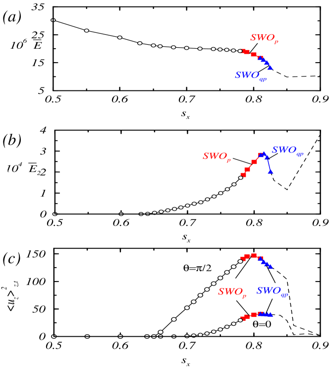
Figure 1: Bifurcations with Niklas parameter $s_{x}$: (a) time-averaged modal kinetic energy, (b) its $m=2$ contribution, and (c) spatiotemporally averaged axial flow field at midgap for $\theta=0$ and $\theta=\pi/2$ in respect of the applied magnetic field. Open and filled symbols are for steady-state and time-dependent solutions, respectively.

Transition to turbulence in ferrofluids.

We first present a sequence of bifurcations with the magnetic parameter $s_{x}$, eventually leading to turbulence. For $s_{x}\neq 0$, the rotating ferrofluid flow is intrinsically three-dimensional AHLL:2010 ; RO:2011 ; ALD:2012 ; ALD:2013 with increased complexity as $s_{x}$ is increased from zero. Figures 1(a-c) show, respectively, three key quantities versus $s_{x}$: the time-averaged modal kinetic energy defined as

$$\sum_{m}\overline{E}_{m}=\left\langle\int_{0}^{2\pi}\int_{-\Gamma/2}^{\Gamma/2}\int_{r_{i}}^{r_{o}}{\bf u}_{m}{\bf u}^{*}_{m}r\textrm{d}r\textrm{d}z\textrm{d}\theta\right\rangle_{t}$$ (7)

its $m=2$ contribution $\overline{E}_{2}$, and the spatiotemporally averaged axial flow field $\langle u_{z}\rangle_{z,t}^{2}$ at midgap for $\theta=0$ (along the magnetic field) and $\theta=\pi/2$ (perpendicular to the field). We see that, for $s_{x}<0.784$, the flow is time-independent. In particular, for $0<s_{x}<s_{x}^{Wt}\approx 0.642$, the flow patterns show wavy vortices with a two-fold symmetry AHLL:2010 , denoted as WVF(2), which appears in Fig. 2(a) as a “two-belly” structure. As $s_{x}$ is increased through $s_{x}^{Wt}$, this symmetry is broken and a somewhat tilting pattern in the wavy-vortex structure emerges [denoted as WVF(2)_t], as shown in Fig. 2(b). The intuitive reason is that the magnetic force is downward for fluid flow near the annulus and upward where the flow exits, resulting in a split in $\langle u_{z}\rangle_{z,t}^{2}$ for $\theta=0$ and $\pi/2$. As $s_{x}$ is increased through the critical point $s_{x}^{p}\approx 0.784$, the flow becomes time-dependent. For $s_{x}\gtrsim s_{x}^{p}$, the flow is time periodic (limit cycle), corresponding to standing waves with axial oscillations of characteristic frequency $\omega_{1}$, which is denoted as SWO_p. Near the onset of SWO_p, the kinetic energy values $\overline{E}$ and $\overline{E}_{2}$ are unaffected, as can be seen from Figs. 1(a) and 1(b), respectively. For $s_{x}\gtrsim s_{x}^{qp}\approx 0.81$, the periodic solution becomes unstable due to the emergence of the second incommensurate frequency $\omega_{2}$ ($\approx\omega_{1}/5$) associated with defect propagation through the annulus in the axial direction, leading to a transition to quasiperiodic flow (denoted as SWO_qp). [See movie files movie1.avi, movie2.avi, movie3.avi, and movie4.avi in Supplementary Materials (SMs), where the additional frequency can be identified visually in the defect starting from the top of the oscillating region, propagating downward toward the bottom, and vanishing there.] While $\overline{E}$ continues to decrease through this transition, both $\overline{E}_{2}$ and $\langle u_{z}\rangle_{z,t}^{2}$ reach their respective maxima at the transition point. As $s_{x}$ is increased further, the flow becomes more complex. Onset of turbulence occurs for $s_{x}\approx s_{x}^{tu}\approx 0.825$, where globally the flow starts to rotate in the azimuthal direction, as shown in Fig. 2(d) (see also movies movie5.avi, movie6.avi, and movie7.avi in SMs). The observed route to turbulence coincides completely with that established previously GS:1975 ; RT:1971 for conventional fluid at high Reynolds numbers.

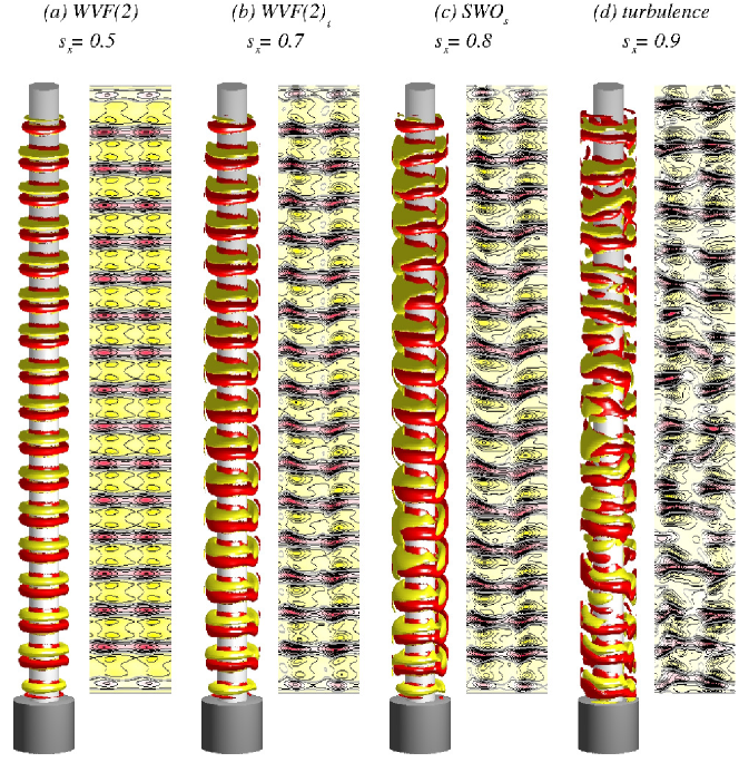
Figure 2: (a-d) For four values of $s_{x}$ corresponding to WVF₂, WVF_t, SWO_p, and turbulence regimes, respectively, isosurfaces of azimuthal vorticity $\eta=\partial_{z}u_{r}-\partial_{r}u_{z}$ and contours of the radial velocity $u_{r}(\theta,z)$ on an unrolled cylindrical surface in the annulus at midgap. Red (dark gray) and yellow (light gray) colors denote $\eta=\pm 100$ for isosurfaces, and inflow and outflow for contour plots, respectively. While the pattern in (a,b) are stationary, the ones in (c,d) are snapshots due to time dependence of the corresponding flow.

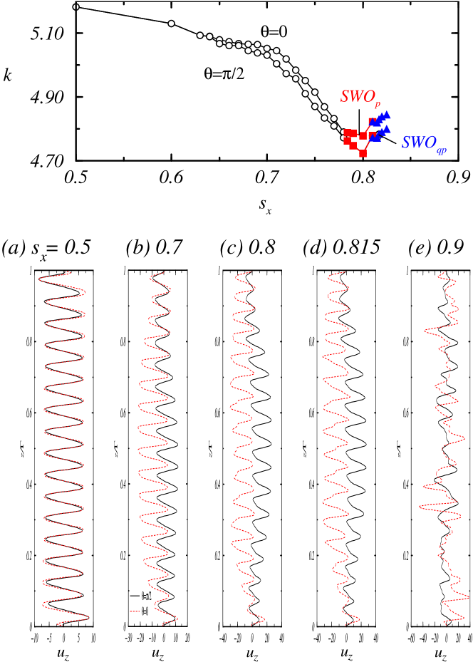
Figure 3: Top panel: variation with $s_{x}$ of the axial wave number $k$ in the directions along ($\theta=0$) and perpendicular to ($\theta=\pi/2$) the magnetic field. (a-e) Snapshots of axial velocity $u_{z}$ for $\theta=0$ (dashed lines) and $\theta=\pi/2$ (solid lines) in the annulus at the midgap location for five different values of $s_{x}$, where (c-e) correspond to periodic, quasiperiodic, and turbulent flows, respectively. The presented patterns are for $m=0$ so that we can identify the largest contribution in the axial Fourier spectrum of $(u_{z})_{0}(z,t)$. In principle one can also identify $k$ from the axial profiles in the figure that gives the axial wavelength $\lambda$ and consequently the wavenumber $k=2\pi/\lambda$. See also movie files movie8.avi, movie9.avi, movie2.avi, movie4.avi and movie7.avi in SMs.

Wave structure of the flows.

We next analyze the wave structure of the flows to probe into the transition to turbulence in the low Reynolds-number regime. To get numerical solutions of the ferrohydrodynamical system, we solve the ferrohydrodynamical system by combining a finite-difference, time-explicit method of second order in $(r,z)$ with Fourier spectral decomposition in $\theta$ (See Method). The variables can be written as

$$f(r,\theta,z,t)=\sum_{m=-m_{\max}}^{m_{\max}}f_{m}(r,z,t)\,e^{im\theta},$$ (8)

where $f$ denotes any one of $\{u_{r},u_{\theta},u_{z},p\}$. We then perform an axial Fourier analysis AHLL:2010 of the mode amplitudes of the radial velocity field $(u_{r})_{m}(z,t)$ at midgap to obtain the behavior of the wave number $k$, as shown in Fig. 3. Prior to the onset of turbulence, the number of vortices in the bulk fluid is invariant, regardless of whether the flow is time-independent or time-dependent. However, due to the symmetry breaking induced by the magnetic field, the spatial structures of the flows can differ significantly. The top panel of Fig. 3 shows that the axial wave number $k$ begins to split into two branches at $s_{x}=s_{x}^{Wt}$, where $k$ is enhanced and reduced as the field enters into and exits perpendicularly from the annulus, respectively, and there are dramatic changes in the flow profiles in which the dynamics tend to focus on the $\theta\approx 0$ region. As $s_{x}$ is increased further, $k$ in the bulk decreases with nearly constant difference between the cases of $\theta=0$ and $\theta=\pi/2$. However, the kinetic energies and the axial wave numbers are nearly unaffected when the flow becomes time-dependent as $s_{x}$ is increased through $s_{x}^{p}$. As the quasiperiodic regime is reached, the energies and the axial wave numbers begin to change where, as shown in Fig. 3, the wave numbers for $\theta=0$ and $\theta=\pi/2$ are minimized at $s_{x}$ about 0.8. For both the periodic and quasiperiodic regimes, there is little variation in $k$ and only the vortex pair surrounding the oscillatory region expands and shrinks periodically. Especially, in the periodic regime the flow profile at $\theta=\pi/2$ exhibits little dependence on $s_{x}$ except for an increasing amplitude, but in the quasiperiodic regime the flow shows a strong dependence on $s_{x}$, due to the emergence of the second frequency. As $s_{x}^{tu}$ is passed, the flow starts to rotate and the split in the axial wave numbers in the directions parallel and perpendicular to the magnetic field vanishes. In fact, as turbulence sets in no distinct wave numbers can be identified, as shown in Figs. 2 and 3(e) (see also movie file movie7.avi in SMs).

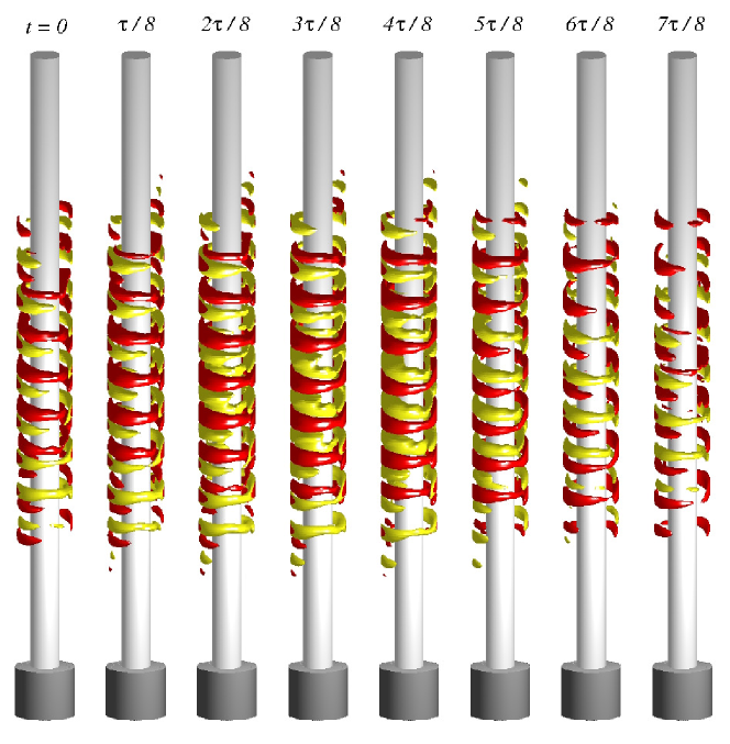
Figure 4: For $s_{x}=0.8$ (periodic regime), isosurfaces of the relative angular momentum $ru_{\theta}-\int_{0}^{\tau}ru_{\theta}dt$ at eight time instants in one period of oscillation, where $\tau\approx 0.058$ and the isolevels are $ru_{\theta}=\pm 5$ (see also movie files movie10.avi, movie11.avi, and movie12.avi in SMs).

Behavior of the angular momentum.

We now examine the behavior of the angular momentum in relation with the flow bifurcation sequence and transition to turbulence. Figure 4 shows, for flows in the periodic regime, the isosurfaces of differences in the angular momentum $ru_{\theta}$ between the full flow and its long-time averaged value, namely, $ru_{\theta}-\int_{0}^{\tau}ru_{\theta}dt$. Onset of the periodic regime can be identified by the occurrence of periodic oscillations (up and down) of a single outward directed jet of angular momentum $ru_{\theta}$ (see movie files movie2.avi, and movie1.avi in SMs). From Fig. 4, we see that, while the full flow pattern in the periodic regime exhibits little variation (see movie files movie10.avi and movie11.avi in SMs), there is relatively large variation in the behavior of the angular momentum (see movie12.avi in SMs). For example, there is a downward flow from $\theta=0$ and an upperward flow from $\theta=\pi$, with opposite angular-momentum values. In the middle of the finite system where the effects of the Ekman boundary layers are minimal, the difference in the angular momentum reaches maximum. As the system enters into the quasiperiodic regime, the appearance of the incommensurate frequency $\omega_{2}$ signifies a kind of defects in the propagation pattern of the flow. As the flow begins to rotate in the azimuthal direction, turbulence sets in.

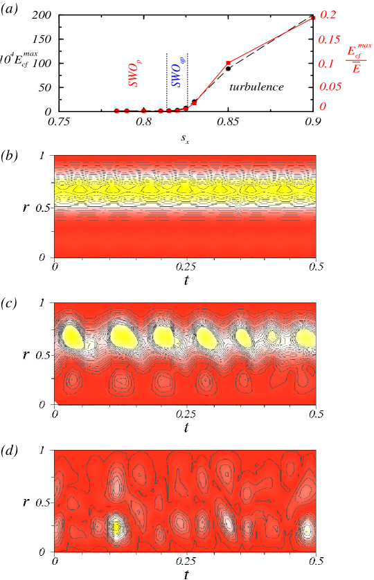
Figure 5: (a) Unnormalized and normalized (by the total kinetic energy) maximum cross-flow energy $E^{max}_{cf}$ versus the Niklas parameter $s_{x}$, where $E_{cf}(r,t)\equiv\langle u_{r}^{2}+u_{z}^{2}\rangle_{A(r)}$ is averaged over the surface of the concentric cylinder. (b-d) Spatiotemporal evolutions of $E_{cf}(r,t)$ for $s_{x}=0.8$, $0.82$, and $0.9$, corresponding to periodic, quasiperiodic, and turbulent regimes, respectively. Red (yellow) color indicates high (low) energy values.

Low Reynolds number turbulence.

An extremely challenging issue in the study of turbulence is precise determination of its onset as a system parameter, e.g., the Reynolds number, is changed. For the type of low-Reynolds number turbulence in ferrofluid uncovered in this Letter, this can actually be achieved. In particular, the transition to turbulence coincides with the onset of azimuthal rotation from the quasiperiodic flow. To illustrate this, we consider the cross-flow energy $E_{cf}(r,t)$, a commonly used indicator for the onset of turbulence in the Taylor-Couette system BE:2013 , which is the instantaneous energy associated with the transverse velocity component at radial distance $r$. Small (large) values of $E_{cf}$ indicate laminar (turbulent) flows. We find that, the maximum value of $E_{cf}(r,t)$, denoted by $E^{max}_{cf}$, assumes near zero values for $s_{x}<s_{x}^{qp}$ but it increases dramatically as $s_{x}$ is increased through $s_{x}^{qp}$, as shown in Fig. 5(a). In this figure we also plot the scaled maximum cross-flow energy value, $E^{max}_{cf}/\overline{E}$, versus $s_{x}$, and we observe that $E^{max}_{cf}$ and $E^{max}_{cf}/\overline{E}$ exhibit essentially the same behavior as the system passes through the onset of turbulence. Examples of the spatiotemporal evolution of $E_{cf}(r,t)$ are shown in Figs. 5(b,c,d) for periodic, quasiperiodic, and turbulent regimes, respectively. We observe regular patterns in the former two regimes, but no apparent patterns in the turbulent regime.

Discussion

To summarize, we have discovered that in the Taylor-Couette ferrofluid system driven by a magnetic field, where flow can exhibit axial oscillations but not rotations in the azimuthal direction in the regular regime, turbulence can generically arise and its onset can occur for low values of the Reynolds number. This is substantiated by extensive computations of the underlying ferrohydrodynamical equation through a systematic bifurcation analysis and characterization of behaviors of physical quantities. The implications, besides the surprising phenomenon of turbulence at very low Reynolds numbers and consequently facilitation of experimental study of turbulence, lie in the perspective of controlled generation of turbulence through variations of the external magnetic field, making it possible to locate the onset of turbulence with high precision. We expect these findings to have values for experimental as well as theoretical investigation of turbulence.

Method

Numerical scheme for ferrodynamical equation.

System (Ferrohydrodynamical equation of motion.) can be solved AHLL:2010 ; ALD:2012 ; ALD:2013 by combining a second-order finite-difference scheme in $(r,z)$ with Fourier spectral decomposition in $\theta$ and (explicit) time splitting. The variables can be written as

$$f(r,\theta,z,t)=\sum_{m=-m_{\max}}^{m_{\max}}f_{m}(r,z,t)\,e^{im\theta},$$ (9)

where $f$ denotes one of $\{u_{r},u_{\theta},u_{z},p\}$. For the parameter regimes considered in our preliminary study, the choice $m_{\max}=10$ provides adequate accuracy. We use uniform grids with spacing $\delta r=\delta z=0.05$ and time-steps $\delta t<1/3800$. For diagnostic purposes, we also evaluate the complex mode amplitudes $f_{m,n}(r,t)$ obtained from the Fourier decomposition in the axial direction $f_{m}(r,z,t)=\sum_{n}f_{m,n}(r,t)e^{inkz}$, where $k$ is the axial wavenumber.

Figure legends

Figure 1: Bifurcations with Niklas parameter $s_{x}$: (a) time-averaged modal kinetic energy, (b) its $m=2$ contribution, and (c) spatiotemporally averaged axial flow field at midgap for $\theta=0$ and $\theta=\pi/2$ in respect of the applied magnetic field. Open and filled symbols are for steady-state and time-dependent solutions, respectively.

Figure 2: (a-d) For four values of $s_{x}$ corresponding to WVF₂, WVF_t, SWO_p, and turbulence regimes, respectively, isosurfaces of azimuthal vorticity $\eta=\partial_{z}u_{r}-\partial_{r}u_{z}$ and contours of the radial velocity $u_{r}(\theta,z)$ on an unrolled cylindrical surface in the annulus at midgap. Red (dark gray) and yellow (light gray) colors denote $\eta=\pm 100$ for isosurfaces, and inflow and outflow for contour plots, respectively. While the pattern in (a,b) are stationary, the ones in (c,d) are snapshots due to time dependence of the corresponding flow.

Figure 3: Top panel: variation with $s_{x}$ of the axial wave number $k$ in the directions along ($\theta=0$) and perpendicular to ($\theta=\pi/2$) the magnetic field. (a-e) Snapshots of axial velocity $u_{z}$ for $\theta=0$ (dashed lines) and $\theta=\pi/2$ (solid lines) in the annulus at the midgap location for five different values of $s_{x}$, where (c-e) correspond to periodic, quasiperiodic, and turbulent flows, respectively. The presented patterns are for $m=0$ so that we can identify the largest contribution in the axial Fourier spectrum of $(u_{z})_{0}(z,t)$. In principle one can also identify $k$ from the axial profiles in the figure that gives the axial wavelength $\lambda$ and consequently the wavenumber $k=2\pi/\lambda$. See also movie files movie8.avi, movie9.avi, movie2.avi, movie4.avi and movie7.avi in SMs.

Figure 4: For $s_{x}=0.8$ (periodic regime), isosurfaces of the relative angular momentum $ru_{\theta}-\int_{0}^{\tau}ru_{\theta}dt$ at eight time instants in one period of oscillation, where $\tau\approx 0.058$ and the isolevels are $ru_{\theta}=\pm 5$ (see also movie files movie10.avi, movie11.avi, and movie12.avi in SMs).

Figure 5: (a) Unnormalized and normalized (by the total kinetic energy) maximum cross-flow energy $E^{max}_{cf}$ versus the Niklas parameter $s_{x}$, where $E_{cf}(r,t)\equiv\langle u_{r}^{2}+u_{z}^{2}\rangle_{A(r)}$ is averaged over the surface of the concentric cylinder. (b-d) Spatiotemporal evolutions of $E_{cf}(r,t)$ for $s_{x}=0.8$, $0.82$, and $0.9$, corresponding to periodic, quasiperiodic, and turbulent regimes, respectively. Red (yellow) color indicates high (low) energy values.

Author contributions

S.A., Y.D. and Y.C.L. devised the research project. S.A. performed numerical simulations. S.A., Y.D. and Y.C.L. analyzed the results. S.A., Y.D. and Y.C.L. wrote the paper.

Additional information

Competing financial interests: The authors declare no competing financial interests.

References

- (1) Gollub, J. P. & Swinney, H. L. Onset of turbulence in a rotating fluid. Phys. Rev. Lett. 35, 927–930 (1975).
- (2) Frisch, U. Turbulence (Cambridge Univ. Press, Cambridge, UK, 1996).
- (3) Tél, T. & Lai, Y.-C. Chaotic transients in spatially extended systems. Phys. Rep. 460, 245–275 (2008).
- (4) Dyke, M. V. An Album of Fluid Motion (The Parabolic Press, Stanford, CA, 1982).
- (5) Gollub, J. P. & Benson, S. V. Many routes to turbulent convection. J. Fluid Mech. 100, 449–470 (1980).
- (6) Franceschini, V. & Zanasi, R. Three-dimensional navier-stokes equations truncated on a torus. Nonlinearity 4, 189–209 (1992).
- (7) Groisman, A. & Steinberg, V. Elastic turbulence in a polymer solution flow. Nature (London) 405, 53–55 (2000).
- (8) Lumley, J. & Blossey, P. Control of turbulence. Annual Review of Fluid Mechanics 30, 311–327 (1998).
- (9) Choi, H. & Moin, P. & Kim, J. Active turbulence control for drag reduction in wall-bounded flows. J. Fluid Mech. 262, 75–110 (1994).
- (10) Taylor, G. I. Stability of a viscous liquid contained between two rotating cylinders. Philos. Trans. R. Soc. London A 223, 289–343 (1923).
- (11) Rosensweig, R. E. Ferrohydrodynamics (Cambridge University Press, Cambridge, UK, 1985).
- (12) Chossat, P. & Iooss, G. The Couette-Taylor Problem (Springer, Berlin, 1994).
- (13) Altmeyer, S. & Hoffmann, C. Secondary bifurcation of mixed-cross-spirals connecting travelling wave solutions. New J. Phys. 12, 113035 (2010).
- (14) DiPrima, R. C. & Swinney, H. L. Instabilities and transition in flow between concentric rotating cylinders (Springer, Berlin, 1985).
- (15) Andereck, C. D., Liu, S. S. & Swinney, H. L. Flow regimes in a circular couette system with independently rotating cylinders. J. Fluid Mech. 164, 155–183 (1986).
- (16) Tagg, R. The couette-taylor problem. Nonlinear Science Today 4, 1–25 (1994).
- (17) Coles, D. Transition in circular couette flow. J. Fluid Mech. 21, 385–425 (1965).
- (18) Shliomis, M. I. Effective viscosity of magnetic suspensions. Sov. JETP 34, 1291 (1972).
- (19) Altmeyer, S., Hoffmann, C., Leschhorn, A. & Lücke, M. Influence of homogeneous magnetic fields on the flow of a ferrofluid in the taylor-couette system. Phys. Rev. E 82, 016321 (2010).
- (20) Reindl, M. & Odenbach, S. Effect of axial and transverse magnetic fields on the flow behavior of ferrofluids featuring different levels of interparticle interaction. Phys. Fluids 23, 093102 (2011).
- (21) Altmeyer, S., Do, Y. & Lopez, J. M. Influence of an inhomogeneous internal magnetic field on the flow dynamics of a ferrofluid between differentially rotating cylinders. Phys. Rev. E 85, 066314 (2012).
- (22) Altmeyer, S., Do, Y. & Lopez, J. M. Effect of elongational flow on ferrofuids under a magnetic field. Phys. Rev. E 88, 013003 (2013).
- (23) Holderied, M., Schwab, L. & Stierstadt, K. Rotational viscosity of ferrofluids and the taylor instability in a magnetic field. Z. Phys. B 70, 431–433 (1988).
- (24) Fauve, S. & Lathrop., D. Laboratory experiments on liquid metal dynamos and liquid metal mhd turbulence. Fluid Dynamics and Dynamos in Astrophysics and Geophysics (2004).
- (25) Shew, W. & Lathro, D. Liquid sodium model of geophysical core convection. Phys. Earth Planet. Inter. 153, 136–149 (2005).
- (26) Wei, X., Jackson, A. & Hollerbach, R. Kinematic dynamo action in spherical couette flow. Geophys. Astrophys. Fluid Dyn. 106, 681–700 (2012).
- (27) Triana, S., Zimmerman, D. & Lathrop, D. Precessional states in a laboratory model of the earth’s core. J. Geophys. Res.-Sol. Ea. 117, B4 (2012).
- (28) Gellert, M., Rüdiger, G. & Hollerbach, R. Helicity and -effect by current-driven instabilities of helical magnetic fields. Monthly Notices Royal Astro. Soc. 414, 2696–2701 (2011).
- (29) Stefani, F. et al. Helical magnetorotational instability in a taylor-couette flow with strongly reduced ekman pumping. Phys. Rev. E 80, 066303 (2009).
- (30) Hollerbach, R., Teeluck, V. & Rüdiger, G. Nonaxisymmetric magnetorotational instabilities in cylindrical taylor-couette flow. Phys. Rev. Lett. 104, 044502 (2010).
- (31) Seilmayer, M., Stefani, F., Gundrum, T., Weier, T. & Gerbeth, G. Experimental evidence for a transient tayler instability in a cylindrical liquid-metal column. Phys. Rev. Lett. 108, 244501 (2012).
- (32) Roach, A. H. et al. Observation of a free-shercliff-layer instability in cylindrical geometry. Phys. Rev. Lett. 108, 154502 (2012).
- (33) Vislovich, A. N., Novikov, V. A. & Sinitsyn, A. K. Influence of a magnetic field on the taylor instability in magnetic fluids. J. Appl. Mech. Tech. Phys. 27, 72–78 (1986).
- (34) Niklas, M. Influence of magnetic fields on taylor vortex formation in magnetic fluids. Z. Phys. B 68, 493–501 (1987).
- (35) Hart, J. E. Ferromagnetic rotating couette flow: The role of magnetic viscosity. J. Fluid Mech. 453, 21–38 (2002).
- (36) Altmeyer, S. Time-dependent ferrofluid dynamics in symmetry breaking transverse. Open J. Fluid Dyn. 3, 116–126 (2013).
- (37) Hollerbach, R. & Fournier, A. End-effects in rapidly rotating cylindrical taylor-couette flow. AIP Conf. Proc. 733, 114–121 (2004).
- (38) Müller, H. W. & Liu, M. Structure of ferrofluid dynamics. Phys. Rev. E 64, 061405 (2001).
- (39) Langevin, P. Magnétisme et théorie des électrons. Annales de Chemie et de Physique 5, 70–127 (1905).
- (40) Embs, J., Müller, H. W., Wagner, C., Knorr, K. & Lücke, M. Measuring the rotational viscosity of ferrofluids without shear flow. Phys. Rev. E 61, R2196–R2199 (2000).
- (41) Niklas, M., Müller-Krumbhaar, H. & Lücke, M. Taylor–vortex flow of ferrofluids in the presence of general magnetic fields. J. Magn. Magn. Mater. 81, 29 (1989).
- (42) Ruelle, D. & Takens, F. On the nature of turbulence. Commun. Math. Phys. 20, 167–192 (1971).
- (43) Brauckmann, H. J. & Eckhardt, B. Intermittent boundary layers and torque maxima in taylor-couette flow. Phys. Rev. E 87, 033004 (2013).