Andreev reflection in edge states of time reversal invariant Landau levels

Abstract

We describe the conductance of a normal-superconducting junction in systems with Landau levels that preserve time reversal symmetry. Those Landau levels have been observed in strained honeycomb lattices. The current is carried along the edges in both the normal and superconducting regions. When the Landau levels in the normal region are half-filled, Andreev reflection is maximal and the conductance plateaus have a peak as a function of filling factor. The height of those peaks is quantized at $4e^{2}/h$. The interface of the junction has Andreev edge states, which form a coherent superposition of electrons and holes that can carry a net valley current. We identify unique experimental signatures for superconductivity in time reversal invariant Landau levels.

Introduction. At zero temperature, Cooper pairs are protected against phase decoherence by time reversal symmetry (TRS). The most promising scenario to study the coexistence of superconductivity and quantum Hall states Tesanovic requires a system that creates well separated Landau levels (LLs) in the complete absence of magnetic flux Uchoa . In strained honeycomb lattices, uniform strain fields can couple to the electrons as a pseudo-magnetic field oriented in opposite directions in the two valleys Guinea ; Low . As observed experimentally in graphene Levy ; Gomes ; Yeh and in deformed honeycomb optical lattices Rechtsman , this field can produce sharp LL quantization, and at the same time, zero net magnetic flux at every lattice site.

In the usual semi-classical picture, electrons moving in cyclotronic orbits are reflected as holes at the interface of a superconductor. At low energy, the holes have opposite momentum (valley) and the same velocity of the incident electrons. Since particle-hole conversion changes the sign of the Lorentz force and effective mass, the Andreev reflected holes and the electrons move coherently in the same direction of the normal-superconducting (NS) interface. The result is an Andreev edge state, a coherent superposition of electrons and holes, which move in alternating skipping orbits along the NS interface Hoppe ; Akhmerov . Pseudo-magnetic fields nevertheless reverse their direction in opposite valleys, preserving TRS. As a consequence, when the energy of the quasiparticles, $\varepsilon$, is small compared to the Fermi energy, $\mu$, reflected holes can retrace the cyclotronic path of the incident electrons, and either form a bound state or counterpropagate along the same insulating edge, as shown in Fig. 1a.

In this Rapid Communications, we study the transport across a NS junction in a honeycomb lattice with a discrete spectrum of TRS LLs. The current is carried through skipping orbits along the edge of the system both in the normalPouyan and in the superconducting regions, as depicted in Fig. 1. We address the regime where the coherence length is longer than the magnetic length. In the limit where the energy of the quasiparticles is small compared to the separation of the LLs, we show that particle-hole conversion produces a peak in each longitudinal conductance plateau. Those peaks are centered around partial filling factors $\nu=4n$, $n\in\mathbb{Z}$, when the normal LLs are half-filled, and their height is quantized at $(n+\frac{1}{2})8e^{2}/h$.

The Andreev edge states carry a finite charge current per valley along the NS interface. The valley current becomes asymptotically small at large energy ($\varepsilon\gg\mu$), when electrons and holes move with the same group velocity. In the opposite regime, $\varepsilon\ll\mu$, electrons and holes have opposite group velocities along the interface, and the valley current is finite. We find transport and spectroscopy signatures that uniquely identify proximity induced superconductivity in TRS LLs Uchoa ; Covaci .

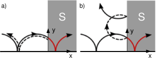
Figure 1: Semi-classical picture of the edge states in TRS LLs at the interface with a superconducting region. Solid black lines: incident electrons with skipping orbits. Red lines: propagating electron pairs at the edge of the superconductor; dashed lines: Andreev reflected holes. a) $\varepsilon\ll\mu$ regime: holes are retroreflected and retrace the path of the incident electrons, preserving their guiding center. They can form a bound state or counterpropagate along the same edge. b) $\varepsilon>\mu$ regime: Andreev holes are specularly reflected and propagate along the NS interface as a superposition of electrons and holes.

Hamiltonian. In the continuum, the electronic Hamiltonian in the presence of a pseudo magnetic-field isAntonio

$$\mathcal{H}_{0}(\mathbf{A})=\left(\begin{array}[]{cc}\mathcal{H}_{+}&0\\ 0&\mathcal{H}_{-}\end{array}\right)=\sum_{\alpha=\pm}\nu_{\alpha}\otimes\mathcal{H}_{\alpha},$$ (1)

where $\nu_{\alpha}=\frac{1}{2}(\nu_{0}+\alpha\nu_{z})$ is the projection operator into the valleys $\alpha=\pm$, and

$$\mathcal{H}_{\alpha}(\mathbf{A})=v(-i\nabla+\alpha\mathbf{A})\cdot\vec{\sigma}_{\alpha}-\mu$$ (2)

is the Dirac Hamiltonian in each valley. $\vec{\sigma}_{\alpha}=(\sigma_{x},\alpha\sigma_{y})$ is a vector of Pauli matrices, $v$ is the Fermi velocity and $\mu$ is the chemical potential.

Near the NS interface, the Bogoliubov-deGennes (BdG) Hamiltonian is

$$\mathcal{H}_{\textrm{BdG}}=\begin{pmatrix}\mathcal{H}_{0}(\mathbf{A})&\hat{\Delta}(\mathbf{r})\\ \hat{\Delta}^{*}(\mathbf{r})&-\mathcal{T}\mathcal{H}_{0}(\mathbf{A})\mathcal{T}^{-1}\end{pmatrix}$$ (3)

where Beenakker2

$$\mathcal{T}=\left(\begin{array}[]{cc}0&\sigma_{z}\\ \sigma_{z}&0\end{array}\right)\mathcal{C}=\nu_{x}\otimes\sigma_{z}\mathcal{C}$$ (4)

is the time reversal symmetry operator, and $\mathcal{C}$ the charge conjugation. Because the field $\mathbf{A}$ preserves TRS, $\mathcal{T}\mathcal{H}_{0}(\mathbf{A})\mathcal{T}^{-1}=\mathcal{H}_{0}(\mathbf{A})$. In a singlet state, the electrons pair symmetrically across the valleys. The simplest Ansatz for the off-diagonal term can be written as Uchoa

$$\hat{\Delta}(\mathbf{r})=\Delta(\mathbf{r})\left(\begin{array}[]{cc}0&\sigma_{0}\\ \sigma_{0}&0\end{array}\right)=\Delta(\mathbf{r})\nu_{x}\otimes\sigma_{0}.$$ (5)

Assuming a sharp NS interface, the superconductor gap varies abruptly at $x=0$,

$$\Delta(\mathbf{r})=\begin{cases}\begin{array}[]{c}\Delta\\ 0\end{array}&\begin{array}[]{c}\mbox{, for $x>0$}\\ ,\mbox{ for }x<0,\end{array}\end{cases}$$ (6)

which separates the normal ($x<0$) from the superconducting region $(x>0$).

In the Landau gauge, $\mathbf{A}=(-By,0)$, the Hamiltonian in the valleys can be written as

$$\mathcal{H}_{\alpha}=\frac{v}{\sqrt{2}\ell_{B}}\alpha\left(i\partial_{\xi}\sigma_{y}+\xi\sigma_{x}\right)-\mu$$ (7)

where $\xi=\ell_{B}k-y/\ell_{B}$ is a dimensionless coordinate with guiding center $X_{\alpha}=\ell_{B}k$, and $\ell_{B}=\sqrt{\hbar/Be}$ is the magnetic length (restoring $\hbar$). By convention, we define the momentum along the edge for each valley as $k_{x}=\alpha k$, with $k>0$. The electronic wavefunction in the normal region moving towards (away from) the interface in valley $\alpha=+$ $(-)$ takes the form $\hat{\psi}_{\alpha}(x,y)=e^{\alpha ikx}\Psi_{\alpha}(y)$, where $\Psi_{\alpha}(y)=(\phi_{A,\alpha},\phi_{B\alpha})$ is a two component spinor in sublattice $A$ and $B$ of the honeycomb lattice.

Edge states. In order describe the edge states, we introduce a mass term potential $M(y)\nu_{0}\otimes\sigma_{z}$, where $M(y)=W$ for $y<0$ and $M=0$ for $y\geq 0$. In the limit $W\to\infty$, this potential describes the edge of the system at $y=0$. The electrons will move in skipping orbits along the $y=0$ line under the influence of a pseudo-magnetic field. In the normal side of the NS interface,

$$\left[\mathcal{H}_{\alpha}+M(y)\sigma_{z}\right]\Psi_{\alpha}=\varepsilon\Psi_{\alpha},$$ (8)

where $\Psi_{\alpha}(y)$ is a two component spinor in the sublattice basis. Multiplying Eq. (8) on the left by the charge conjugated form of $\mathcal{H}_{\alpha}+M(y)\sigma_{z}$, where $\mu\to-\mu$, this equation assumes a diagonal form,

$$\left[\frac{1}{2}\partial_{\xi}^{2}-\frac{1}{2}\xi^{2}-M^{2}(y)+(\varepsilon+\mu)^{2}-\frac{1}{2}\sigma_{z}\right]\Psi_{\alpha}=0.$$ (9)

For $y\geq 0$, where $M=0$, the energy spectrum of the LLs at the edge is

$$\epsilon(k_{x})=s(\sqrt{2}v/\ell_{B})\sqrt{|n(k_{x})|}-\mu$$ (10)

where $n(k_{x})$ is a real number and $s=\mbox{sign}[n(k_{x})]$. The corresponding eigenvectors in the two valleys are of the form

$$\Psi_{\alpha,n}(\xi)=\left(\begin{array}[]{c}D_{n(k_{x})-1}\left(\frac{\xi}{\sqrt{2}}\right)\\ s\alpha D_{n(k_{x})}\left(\frac{\xi}{\sqrt{2}}\right)\end{array}\right),$$ (11)

where $D_{n(k_{x})}(x)$ are parabolic cylinder functions. The determination of $n(k_{x})$ follows from enforcing boundary conditions at the edge and results in a discrete number of edge states shown in Fig. 2a. For definiteness, we consider the case of a zigzag edge, where $\phi_{B,+}(k\ell_{B}/\sqrt{2})=0$, although similar conclusions apply to any choice of boundary conditions.

Figure 2: Energy spectrum versus guiding center $k_{x}\ell_{B}$ at the edge ($y=0$) for $\mu=1.5$ ($\nu=4$) and $\Delta=0.5$. Energy scales in units of $\sqrt{2}v/\ell_{B}$. a) Normal region ($x<0$). b) superconducting region ($x>0$).

In the superconducting region, we can decompose the BdG Hamiltonian (3) into two identical blocks of $4\times 4$ matrices, where

$$\begin{pmatrix}\mathcal{H}_{\alpha}&\Delta\sigma_{0}\\ \Delta^{*}\sigma_{0}&-\mathcal{H}_{\alpha}\end{pmatrix}\Phi_{\alpha}=E\Phi_{\alpha},$$ (12)

is the reduced BdG equation and $\Phi_{\alpha}=(\Psi_{e,\alpha}\Psi_{h,\alpha})$ is a $4$ component spinor including electron and hole states. At $y>0$, where the wavefunctions are finite ($M=0$), the solution follows from squaring (12) with the charge conjugated BdG Hamiltonian, which results in the differential equation

$$\left[\frac{1}{2}\partial_{\xi}^{2}-\frac{1}{2}\xi^{2}+\epsilon^{2}+\mu^{2}+\Delta^{2}+2\mu\mathcal{M}\right]\Phi_{\alpha}=0,$$ (13)

where

$$\mathcal{M}=\left(\begin{array}[]{cc}\epsilon-\frac{1}{2}\sigma_{z}&-\Delta\sigma_{0}\\ -\Delta\sigma_{0}&-\epsilon-\frac{1}{2}\sigma_{z}\end{array}\right)$$

is a 4$\times 4$ matrix in the particle-hole basis, and $\Delta$ is assumed real. The four component spinor that satisfies Eq. (13) and hence (12) is

$$\Phi_{\alpha}=\left(\begin{array}[]{c}\beta_{\alpha}\Psi_{\alpha,n_{s}}(\xi)\\ \beta_{-\alpha}\Psi_{\alpha,n_{s}}(\xi)\end{array}\right)$$ (14)

where $\beta_{\alpha}=\sqrt{\frac{1}{2}(1+\alpha\sqrt{1-\Delta^{2}/E^{2}})}$, with $\alpha=\pm$ indexing the valleys. The energy spectrum in the superconducting edge is given by

$$E(k_{x})=\sqrt{\left(\bar{s}(\sqrt{2}v/\ell_{B})\sqrt{|n_{s}(k_{x})|}-\mu\right)^{2}+\Delta^{2}},$$ (15)

where $\bar{s}=\mbox{sign}[n_{s}(k_{x})]$ and $n_{s}(k_{x})$ is a real number to be found from the boundary condition at the edge ($y=0$), in superconducting side. Imposing similar boundary conditions $\phi_{B,+}(k\ell_{B}/\sqrt{2})=0$, the energy spectrum at the superconducting edge is shown in Fig. 2b.

Transport across the NS junction. In the normal region, the electron and hole like excitations are decoupled. Near the NS interface, the normal edge state can be written as a superposition of the wavefunctions of the incident electron, $\psi_{e}^{+}(x,y)$, the reflected electron in the opposite valley, $\psi_{e}^{-}(x,y)$, and the Andreev reflected hole, $\psi_{h}^{-}(x,y)$. For simplicity, we assume from now on all length scales to be in units of the magnetic length $\ell_{B}$ and all energy scales to be in units of $\sqrt{2}v/\ell_{B}$.

The largest contribution to scattering comes from states at integer values of $n(k)$ and $n_{s}(k)$, where the density of states is the largest. In the four component particle-hole basis, the electron wavefunctions are

$$\psi_{e,i}^{+}(x,y)=\left(\begin{array}[]{c}\Psi_{+,n_{e}}\left(k_{i}-y\right)\\ \mathbf{0}\end{array}\right)e^{ik_{i}x},$$ (16)

and

$$\psi_{e,i}^{-}(x,y)=\sum_{j}^{C_{n_{e}}}r_{i,j}^{e}\left(\begin{array}[]{c}\Psi_{-,n_{e}}\left(k_{j}-y\right)\\ \mathbf{0}\end{array}\right)e^{-ik_{j}x},$$ (17)

where the nearest integer function $n_{e}=\mbox{nint}\!\left[(\epsilon+\mu)^{2}\right]\in\mathbb{Z}$ sets the index of the highest occupied band, with $C_{n_{e}}=2n_{e}+1$ the number of channels crossing the Fermi level at the edge. The wavefunction of the Andreev reflected hole is

$$\psi_{h,i}^{-}(x,y)=\sum_{j}^{C_{n_{h}}}r_{i,j}^{A}\left(\begin{array}[]{c}\mathbf{0}\\ \Psi_{-,n_{h}}\left(k_{j}-y\right)\end{array}\right)e^{-ik_{j}x},$$ (18)

where $n_{h}=\mbox{nint}\!\left[(\epsilon-\mu)^{2}\right]\in\mathbb{Z}$, with $C_{n_{h}}$ equivalently the number of edge channels for hole states.

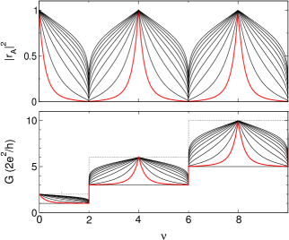
Figure 3: Top panel: Andreev reflected hole probability $|r_{A}|^{2}$ per channel as a function of the normal filling factor $\nu$. The superconductor gap $\Delta$ (in units of $\sqrt{2}v/\ell_{B}$) ranges from $0.01$ (red line) to $0.2$ in steps of $0.025$. Bottom: corresponding longitudinal conductance $G$ at the edge as a function of $\nu$. The solid line plateaus: normal conductance ($\Delta=0$). Dotted lines: upper bound for the conductance, which is quantized at $4e^{2}/h$. In all curves, the temperature $T=0.02(\sqrt{2}v/\ell_{B})$.

In the superconducting region, the electron-like and hole-like solutions can be written as,

$$\psi_{S,i}^{\alpha}=\sum_{j}^{C_{n_{\alpha}}}A_{i,j}^{\alpha}\left(\begin{array}[]{c}\beta_{\alpha}\Psi_{\alpha,n_{+}}\left(k_{j}-y\right)\\ \beta_{-\alpha}\Psi_{\alpha,n_{+}}\left(k_{j}-y\right)\end{array}\right)e^{\alpha ik_{j}x},$$ (19)

where $n_{\alpha}=\mbox{nint}[\left(\sqrt{E^{2}-\Delta^{2}}+\alpha\mu\right)^{2}]\in\mathbb{Z}$. The reflected electron and hole amplitudes can be calculated by matching the amplitudes at the interface ($x=0$),

$$\psi_{e}^{+}+\psi_{e}^{-}+\psi_{h}^{-}=\psi_{S}^{+}+\psi_{S}^{-}.$$ (20)

In the limit of large coherence length, $\xi=v/\Delta\gg\ell_{B}$, and $\epsilon\ll v/\ell_{B}$, we can neglect scattering processes between different modes. Also, the number of edge channels is the same for electrons and holes in the two sides of the junction, $n_{e}=n_{h}=n_{\alpha}$. In this regime, the solution of Eq. (20) is $r_{i}^{e}=0$ and $r_{i}^{A}=\beta_{+}/\beta_{-}=E/\Delta-\sqrt{E^{2}/\Delta^{2}-1}$. When $E<\Delta$, $r_{i}^{A}$ is complex and the total amplitude of the Andreev reflection is $|r_{i}^{A}|^{2}=1$.

In fig. 3, we show the amplitude of the Andreev reflection versus the filling factor of the normal LLs. In the normal region, when the LLs are well separated, the Fermi distribution of the quasiparticles is equal to the filling fraction of the highest occupied LL, $(\mbox{e}^{\epsilon/T}+1)^{-1}=f(\nu)=(\nu/4+\frac{1}{2})\mbox{mod}(1)\in[0,1]$, where $T$ is the temperature. The Andreev amplitude is $r_{i}^{A}\equiv\Theta(\nu)$, where

$$\Theta(\nu)=-\frac{|\epsilon(\nu)|}{\Delta}+\sqrt{\frac{\epsilon^{2}(\nu)}{\Delta^{2}}+1},$$ (21)

with

$$\epsilon(\nu)=T\ln\left(\frac{f(\nu)}{1-f(\nu)}\right).$$ (22)

From the Blonder-Tinkham-Klapwijk formula Blonder , the differential conductance at the NS junction can be written as

$$G=\frac{2e^{2}}{h}\sum_{i=1}^{C_{n}}(1-|r_{i}^{e}|^{2}+|r_{i}^{A}|^{2})\approx\frac{4e^{2}}{h}\!\left(\!n+\frac{1}{2}\right)\!\!\left[1+|\Theta(\nu)|^{2}\right]\!.$$ (23)

The peaks in the differential conductance are shown in the bottom panel of Fig. 3 as a function of the filling factor of the normal region $\nu$. The solid line plateaus represent the conductance in the absence of Andreev reflections. The different curves show the conductance for different values of the normalized gap $\Delta$ ranging from $0.01$ (red line) to 0.2 in $0.025$ steps. The peaks appear at partial fillings $\nu=4n$, $n\in\mathbb{Z}$, and their height is quantized at $(2n+1)4e^{2}/h$. At those fillings, the normal LLs are particle-hole symmetric and Andreev reflection is maximal. At integer fillings $\nu=4(n+\frac{1}{2})$, when the Fermi level is in the middle of the LL gap, Andreev reflection is suppressed and the conductance is quantized by half, at $(2n+1)2e^{2}/h$.

Figure 4: Energy spectrum $\varepsilon$ along the NS interface ($x=0$) versus guiding center $k_{y}\ell_{B}$. Negative guiding centers ($k_{y}\ell_{B}<0$) describe states in the normal region. $k_{y}\ell_{B}>0$ correspond to states in the superconducting one. Left curves: normal edge states. Center right curves: low energy Andreev edge states. a) $\mu=0$ $(\nu=0$), $\varepsilon>\mu$ regime for finite $\Delta$. Electron and hole states have the same group velocity $v_{g}=\mbox{d}\varepsilon/\mbox{d}k_{y}$ and propagate in the same direction of the interface; b) $\mu/\Delta=2$: electrons and Andreev reflected holes have the same guiding center and opposite group velocities along the interface for $\varepsilon\ll\mu$, forming an Andreev bound state.

Andreev edge states. More insight on Andreev reflection and the electronic states near the interface can be obtained by considering the current flowing parallel to the interface. In the configuration where the insulating edge is zigzag, the NS interface has armchair character. Its states are formed by a superposition of eigenstates on both valleys. Using the Landau gauge $\mathbf{A}=(0,Bx)$, the wavefunction in the normal side of the interface can be written as

$$\psi_{\parallel}(x,y)=\sum_{\alpha}\left(\begin{array}[]{c}a_{e,\alpha}\Psi_{\alpha,n_{e}(\varepsilon)}\left(x-k_{y}\right)\\ a_{h,\alpha}\Psi_{\alpha,n_{h}(\varepsilon)}\left(x-k_{y}\right)\end{array}\right)e^{\alpha ik_{y}y},$$ (24)

where $n_{e}(\varepsilon)=(\varepsilon+\mu)^{2}$ and $n_{h}(\varepsilon)=(\varepsilon-\mu)^{2}$ are real numbers. In the superconducting side,

$$\psi_{S\parallel}(x,y)=\sum_{\alpha,\gamma}A_{\parallel,\gamma}^{\alpha}\left(\begin{array}[]{c}\beta_{\gamma}\Psi_{\alpha,n_{\alpha}(\varepsilon)}\left(x-k_{y}\right)\\ \beta_{-\gamma}\Psi_{\alpha,n_{\alpha}(\varepsilon)}\left(x-k_{y}\right)\end{array}\right)e^{\alpha ik_{y}y},$$ (25)

with $\gamma=+$$(-)$ indexing electron(hole)-like states, and $n_{\alpha}(\varepsilon)=\left(\sqrt{\varepsilon^{2}-\Delta^{2}}+\alpha\mu\right)^{2}$. Matching the amplitudes $\psi_{\parallel}(0,y)=\psi_{S\parallel}(0,y)$ and the derivatives $\partial_{x}\psi_{\parallel}(x,y)=\partial_{x}\psi_{S\parallel}(x,y)$ at $x=0$ yields eight linear equations for eight unknown coefficients $\mathcal{V}_{i}$, with $i=1,\ldots,8$. This set of equations can be expressed in matrix form as $\mathcal{Q}\cdot\mathcal{V}=0$. Non-trivial solutions require that $\mbox{Det}(\mathcal{Q})=0$. From this condition, we numerically extract the spectrum of excitations $\varepsilon(k_{y})$ near the NS interface, as shown in Fig. 4.

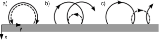
Figure 5: Andreev edge states at the NS interface. Solid lines: electron cyclotronic orbits; dashed: Andreev reflected holes. a) $\varepsilon/\mu\to 0$ regime: electrons and holes form a bound state. b) Intermediate regime, $\varepsilon<\mathrm{min}(\mu,\Delta)$: electrons are retroreflected into holes with group velocity $v_{g}=\partial\varepsilon/\partial k_{y}$ having opposite sign. c) $\varepsilon>\mu$ regime: electrons are specularly reflected into holes, which propagate along the same direction.

The interface states are an admixture of two type of modes: i) normal edge states formed by conventional skipping orbits moving in one direction, and ii) Andreev states, which are coherent superpositions of particles and holes. The first mode is connected to bulk LL energies in the normal region as $k_{y}\rightarrow-\infty$. The second one has no correspondence with the bulk LLs in the normal region, and appears around $k_{y}\ell_{B}\sim 0$ and also inside the superconducting region, for positive guiding centers ($k_{y}>0$).

In panel 4a, we plot the interface modes at $\mu=0$ ($\nu=0$), for finite $\Delta$. In this regime, $\varepsilon>\mu=0$, the group velocity of the Andreev edge states $v_{g}=\partial\varepsilon/\partial k_{y}>0$ for both electrons and holes (center right curves), which are specularly reflected at the interface Beenakker and move in alternating skipping orbits in the same direction (see fig. 5c). In the limit $\varepsilon\gg\mu$ , electrons and holes have the same velocity and guiding center, and carry zero net charge per valley. In all other cases, their velocities are different, resulting in a net valley current along the NS interface. In panel 4b, we plot the energy of the modes for $\mu/\Delta=2$. In the regime $\varepsilon<\mathrm{min}(\mu,\Delta)$ we find numerically that the Andreev reflected holes and electrons have group velocities $v_{g}$ with opposite signs (fig. 5b). In the limit $\varepsilon/\mu\to 0$, the holes retrace the path of the incident electrons, forming an Andreev bound state schematically shown in fig. 5a.

In summary, we have derived transport and spectroscopy signatures of proximity induced superconductivity in TRS LLs. We found the longitudinal conductance as a function of the filling factor across an NS junction, and showed that it is quantized at $(2n+1)4e^{2}/h$ in the $n$-th LL at half-filling, when Andreev reflection is maximal. We also showed that the NS interface has Andreev edge states, with unique spectroscopic features.

Acknowledgements. We thank K. Mullen and P. Carmier for discussions. BU acknowledges University of Oklahoma and NSF Career grant DMR-1352604 for support.

References

(1)Z. Tesanovic, M. Rasolt, L. Xing, Phys. Rev. Lett.
63, 2425 (1993).
(2)B. Uchoa and Y. Barlas, Phys. Rev. Lett 111,
046604 (2013).
(3)F. Guinea, M. I. Katsnelson and A. K. Geim, Nat.
Phys. 6, 30 (2010).
(4)Tony Low, and F. Guinea, Nanoletters 10, 3551
(2010).
(5)N. Levy, S. A. Burke, K. L. Meaker, M. Panlasigui,
A. Zettl, F. Guinea, A. H. C. Neto, and M. F. Science 329,
544 (2010).
(6)K. K. Gomes, W. Mar, W. Ko, F. Guinea, and H. C. Manoharan,
Nature 483, 306 (2012).
(7)N.-C. Yeh, M.-L. Teague, S. Yeom, B. L. Standley, R.
T.-P. Wu, D. A. Boyd, and M. W. Bockrath, Surf. Sci. 605, 1649 (2011).
(8)M. C. Rechtsman, J. M. Zeuner, A. Tünnermann,
S. Nolte, M. Segev and A. Szameit, Nat. Photonics 7, 153
(2013).
(9)H. Hoppe, U. Z licke, and Gerd Sch n, Phys. Rev. Lett.
84, 1804 (2000).
(10)A. R. Akhmerov and C. W. J. Beenakker, Phys. Rev.
Lett. 98, 157003 (2007).
(11)P. Ghaemi, S. Gopalakrishnan, and S. Ryu, Phys. Rev. B 87, 155422 (2013).
(12)L. Covaci and F. M. Peeters, Phys. Rev. B 84,
241401(R) (2011).
(13)A. H. Castro Neto, N. M. R. Peres, F. Guinea, K.
Novoselov, A. Geim, Rev. Mod. Phys. 81, 109 (2009).
(14)C. W. J. Beenakker, Rev. Mod. Phys. 80,
1337 (2008).
(15)G. E. Blonder, M. Tinkham, and T. M. Klapwijk, Phys.
Rev. B 25, 4515 (1982).
(16)C. W. J. Beenakker, Phys. Rev. Lett. 97,
067007 (2006).