Electromagnetic and neutral-weak response functions of ⁴He and ¹²C

Abstract

Ab initio calculations of the quasi-elastic electromagnetic and neutral-weak response functions of ⁴He and ¹²C are carried out for the first time. They are based on a realistic approach to nuclear dynamics, in which the strong interactions are described by two- and three-nucleon potentials and the electroweak interactions with external fields include one- and two-body terms. The Green’s function Monte Carlo method is used to calculate directly the Laplace transforms of the response functions, and maximum-entropy techniques are employed to invert the resulting imaginary-time correlation functions with associated statistical errors. The theoretical results, confirmed by experiment in the electromagnetic case, show that two-body currents generate excess transverse strength from threshold to the quasi-elastic to the dip region and beyond. These findings challenge the conventional picture of quasi-elastic inclusive scattering as being largely dominated by single-nucleon knockout processes.

In first-order perturbation theory, the interactions of an external electroweak probe with a nucleus are described by response functions. These response functions—two for the processes $A(e,e^{\prime})$ induced by electromagnetic interactions, and five for the processes $A(\nu_{l},\nu_{l}^{\prime})$ and $A(\overline{\nu}_{l},\overline{\nu}_{l}^{\,\prime})$, or $A(\nu_{l},l^{-})$ and $A(\overline{\nu}_{l},l^{+})$, induced by neutral or charge-changing weak interactions—determine the inclusive differential cross sections Shen et al. (2012). They can be written schematically as

$$R_{\alpha\beta}(q,\omega)\!\sim\!\sum_{f}\delta(\omega+E_{0}-E_{f})\langle f|O_{\alpha}({\bf q})|0\rangle^{*}\langle f|O_{\beta}({\bf q})|0\rangle,$$ (1)

where ${\bf q}$ and $\omega$ are the momentum and energy transfers injected by the external field into the nucleus, $|0\rangle$ and $|f\rangle$ represent respectively its initial ground state of energy $E_{0}$ and final continuum state of energy $E_{f}$, $O_{\alpha}({\bf q})$ and $O_{\beta}({\bf q})$ denote appropriate components of the of the nuclear electroweak current operator (their $\omega$-dependence is dealt with as described below), and an average over the ground-state spin projections is understood (precise definitions for the nuclear electroweak response functions, and resulting inclusive cross sections, are given in Ref. Shen et al. (2012)).

At large values of momentum and energy transfers ($q\gtrsim 1$ GeV and $\omega\gtrsim 0.5$ GeV), where the dynamics of interacting nucleons is inextricably interwoven with the internal dynamics of individual nucleons, the accurate calculation of the response functions poses formidable challenges, particularly in view of the fact that a consistent theoretical framework to describe such a regime is still lacking. Even at the lower $q$ and $\omega$ of interest in the present study ($q\lesssim 0.5$ GeV and $\omega$ in the quasi-elastic region), where the consequences of the nucleon’s substructure on nuclear dynamics can be subsumed into effective many-body potentials and currents, this calculation remains extremely difficult: it requires knowledge of the whole excitation spectrum of the nucleus and inclusion in the electroweak currents of one- and many-body terms.

In the case of inclusive weak scattering, a further difficulty exists for comparing calculated and experimental results. The experimental initial neutrino energy is not known; instead there is a broad spectrum of energies. This means that the observed cross section for a given energy and angle of the final lepton follows from a folding with the energy distribution of the incoming neutrino flux and, consequently, may include contributions from $q$-$\omega$ regions where different mechanisms are at play: the threshold region, where the structure of the low-lying energy spectrum and collective effects are important; the quasi-elastic region, which is dominated by scattering off individual nucleons and nucleon pairs (see below); and the $\Delta$-resonance region, where one or more pions are produced in the final state Benhar (2012).

Integral properties of the response functions can be studied by means of sum rules, which are obtained from ground-state expectation values of appropriate combinations of the current operators (and commutators of these combinations with the Hamiltonian in the case of energy-weighted sum rules), thus avoiding the need for computing the nuclear excitation spectrum. Ab initio quantum Monte Carlo (QMC) calculations of (non-energy-weighted) electroweak sum rules in ¹²C have been recently reported in Refs. Lovato et al. (2013, 2014). These calculations have demonstrated that a large fraction ($\simeq 30$%) of the strength in the response arises from processes involving two-body currents, and that interference effects between the matrix elements of one- and two-body currents play a major role Benhar et al. (2013). These effects are typically only partially, or approximately, accounted for in existing perturbative or mean-field studies Martini et al. (2009, 2010); Nieves et al. (2011); Amaro et al. (2011).

Yet, sum rules do not provide direct information on the distribution of strength, whether, for example, the calculated excess strength induced by two-body currents is mostly at large $\omega$, well beyond the quasi-elastic peak energy $\omega_{\rm qe}=\sqrt{q^{2}+m^{2}}-m$ ($m$ is the nucleon mass), or is also found in the quasi-elastic region with $\omega\lesssim\omega_{\rm qe}$. Moreover, in the electromagnetic case, comparison of theoretical and experimental sum rules is problematic, since longitudinal and transverse response functions obtained from Rosenbluth separation of measured inclusive $(e,e^{\prime})$ cross sections are only available in the space-like region ($\omega<q$) and therefore must be extrapolated into the unobserved time-like region ($\omega>q$) before “experimental” values for the sum rules can be determined, see Refs. Lovato et al. (2013); Carlson et al. (2002) for a discussion of these issues.

In this paper we report the first ab initio calculations of the electromagnetic and neutral-weak response functions of ⁴He and ¹²C (other studies for ⁴He have been already performed within different frameworks, i.e. Leidemann and Orlandini (2013); Bacca et al. (2009)). These calculations proceed in two steps: the first involves the use of QMC methods to compute the response in imaginary time, the so-called Euclidean response Carlson and Schiavilla (1992, 1994), while the second consists in the inversion, via maximum entropy techniques Bryan (1990); Jarrell and Gubernatis (1996), of these “noisy” imaginary-time data to obtain $R_{\alpha\beta}(q,\omega)$. The dynamical framework is based on a realistic Hamiltonian, including the Argonne $v_{18}$ two-nucleon Wiringa et al. (1995) (AV18) and Illinois-7 three-nucleon Pieper (2008) (IL7) potentials, and on realistic electroweak currents with one- and two-body terms. A concise description of this framework is in Refs. Lovato et al. (2013, 2014), while a more extended one can be found in the reviews Carlson and Schiavilla (1998); Carlson et al. (2014). These latter papers also illustrate the level of quantitative success it has achieved in accurately predicting many properties of s- and p-shell nuclei up to ¹²C, including, among others, energy spectra of low-lying states, static properties like charge radii, magnetic dipole and electric quadrupole moments, radiative and weak transition rates, and elastic and inelastic electromagnetic form factors.

The Euclidean response function is defined as the Laplace transform

$$E_{\alpha\beta}(q,\tau)=C_{\alpha\beta}(q)\int_{\omega_{\rm th}}^{\infty}d\omega\,e^{-\tau\omega}R_{\alpha\beta}(q,\omega)\ ,$$ (2)

where $\omega_{\rm th}$ is the inelastic threshold and the $C_{\alpha\beta}$ are $q$-dependent normalization factors. In $R_{\alpha\beta}(q,\omega)$ the $\omega$-dependence enters via the energy-conserving $\delta$-function and the dependence on the four-momentum transfer $Q^{2}=q^{2}-\omega^{2}$ of the electroweak form factors of the nucleon and $N$-to-$\Delta$ transition in the currents. We remove the latter by evaluating these form factors at $Q^{2}_{\rm qe}=q^{2}-\omega_{\rm qe}^{2}$. In the case of the electromagnetic longitudinal ($L$ or $\alpha\beta=00$) and transverse ($T$ or $\alpha\beta=xx$) response functions, the normalization factors are Carlson et al. (2002) $C_{L}=C_{T}=1/\left[G_{E}^{p}(Q^{2}_{\rm qe})\right]^{2}$, where $G_{E}^{p}$ is the proton electric form factor, while in the neutral-weak response functions they are the same as those adopted in the sum rule calculations reported in Ref. Lovato et al. (2014). With these definitions the response functions in Eq. (2) can be thought of as being due to point-like, but strongly interacting, nucleons. Note that non-energy-weighted sum rules Lovato et al. (2013, 2014) correspond to $E_{\alpha\beta}(q,\tau\!=\!0)$, while energy-weighted ones are obtained by taking derivatives of $E_{\alpha\beta}(q,\tau)$ with respect to $\tau$ and evaluating them at $\tau=0$.

The Euclidean response can be expressed as a ground-state expectation value,

$$\frac{E_{\alpha\beta}(q,\tau)}{C_{\alpha\beta}(q)}=\frac{\langle 0|O^{\dagger}_{\alpha}({\bf q})e^{-(H-E_{0})\tau}O_{\beta}({\bf q})|0\rangle}{\langle 0|e^{-(H-E_{0})\tau}|0\rangle}\ ,$$ (3)

where $H$ is the nuclear Hamiltonian (here, the AV18/IL7 model), $\tau$ is the imaginary-time, and $E_{0}$ is a trial energy to control the normalization. In this paper we report responses computed with the variational wave function, $|0\rangle=|\Psi_{V}\rangle$; in Refs. Lovato et al. (2013, 2014) it was shown that sum rules computed with $|\Psi_{V}\rangle$ are very close to those computed with the exact Green’s function Monte Carlo (GFMC) wave functions. The calculation of the matrix element above is carried out with GFMC methods Carlson and Schiavilla (1992) similar to those used in projecting out the exact ground state of $H$ from a trial state Carlson (1987). It proceeds in two steps. First, an unconstrained imaginary-time propagation of the variational Monte Carlo (VMC) state $|\Psi_{V}\rangle$ is performed and saved. Next, the states $O_{\beta}({\bf q})|\Psi_{V}\rangle$ are evolved in imaginary time following the path previously saved. During this latter imaginary-time evolution, scalar products of ${\rm exp}\left[-\left(H-E_{0}\right)\tau_{i}\right]O_{\beta}({\bf q})|\Psi_{V}\rangle$ with $O_{\alpha}({\bf q})|\Psi_{V}\rangle$ are evaluated on a grid of $\tau_{i}$ values, and from these scalar products estimates for $E_{\alpha\beta}(q,\tau_{i})$ are obtained (a complete discussion of the methods is in Refs. Carlson and Schiavilla (1992); Carlson et al. (2002)).

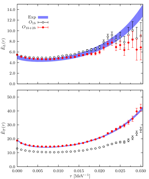
Figure 1: (Color online) Euclidean electromagnetic longitudinal (top panel) and transverse (lower panel) response function of ¹²C at $q=570$ MeV. Experimental data are from Ref. Jourdan (1996).

In Fig. 1 the electromagnetic longitudinal ($E_{L}$, top panel) and transverse ($E_{T}$, lower panel) Euclidean response functions of ¹²C are compared to those extracted from the world data analysis by Jourdan Jourdan (1996), represented by the shaded bands. In order to better show the large $\tau$ behavior, all the figures in this paper show $\widetilde{E}_{\alpha\beta}(q,\tau)=\exp[\tau\,q^{2}/(2m)]E_{\alpha\beta}(q,\tau)$; this scaled response would be a constant for an isolated proton. The “experimental” $E_{L}(q,\tau)$ and $E_{T}(q,\tau)$ follow from Laplace-transforming the longitudinal and transverse data. These are first divided by $\left[G_{E}^{p}(Q^{2})\right]^{2}$ to obtain corresponding response functions of point-like nucleons, and then integrated with the weight factor ${\rm exp}(-\tau\omega)$ up to $\omega_{\rm max}$, where measurements are available. The strength in the unobserved region with $\omega>\omega_{\rm max}$ is estimated by assuming that the $R_{L}(q,\omega>\omega_{\rm max})$ and $R_{T}(q,\omega>\omega_{\rm max})$ of ¹²C are proportional to those in the deuteron, which can be accurately calculated Shen et al. (2012). The procedure is identical to that used in Ref. Lovato et al. (2013) for the sum rules. As discussed in Ref. Lovato et al. (2013), the scaling assumption can be justified by observing that the high $\omega$ (well beyond $\omega_{\rm qe}$) region of the response is dominated by two-nucleon physics, in particular by deuteron-like $np$ pairs in the ground-state of the nucleus. It is important to stress that, as $\tau$ increases, the Euclidean response functions become more and more sensitive to strength in the quasi-elastic and threshold regions of $R_{L,T}(q,\omega)$. Indeed, in this limit ($\tau\gtrsim 1/\omega_{\rm qe}$) contributions from unmeasured strength at $\omega>\omega_{\rm max}$ are exponentially suppressed.

In Fig. 1 we show results obtained by including only one-body (open circles) or both one- and two-body (solid circles) terms in the electromagnetic transition operators. In the longitudinal case, destructive interference between the matrix elements of the one- and two-body charge operators reduces, albeit slightly, the one-body response. In the transverse case, on the other hand, two-body current contributions substantially increase the one-body response. This enhancement is effective over the whole imaginary-time region we have considered, with the implication that excess transverse strength is generated by two-body currents not only at $\omega\gtrsim\omega_{\rm qe}$, but also in the quasi-elastic and threshold regions of $R_{T}(q,\omega)$. It is reassuring to see that the full predictions for both longitudinal and transverse Euclidean response functions are in excellent agreement with data.

At larger values of $\tau$ the statistical errors associated with the GFMC evolution are rather large, particularly in the longitudinal response for which the elastic contribution proportional to the square of the ¹²C form factor Lovato et al. (2013) needs to be removed in order to account for the inelastic strength only. However, it should be possible to reduce these errors in the future by investing substantial additional computational resources in this type of calculation. Those presented here were performed with $\sim$45 million core hours of Argonne National Laboratory’s IBM Blue Gene/Q (Mira) parallel supercomputer. The Automatic Dynamic Load Balancing (ADLB) library Lusk et al. (2010) was used to distribute the imaginary time propagation of $O_{\beta}(\mathbf{q})|\Psi_{V}\rangle$ and the evaluation of the matrix element in Eq. (3) over more than 8000 MPI ranks. The code is at present approximately 75% efficient at this scale.

In Fig. 2 we show the largest of the five Euclidean neutral-weak response functions: the transverse (top panel) and interference (lower panel) $E_{\alpha\beta}(q,\tau)$, having respectively $\alpha\beta=xx$ and $\alpha\beta=xy$ in the notation of Ref. Shen et al. (2012). The $E_{xy}(q,\tau)$ response is due to interference between the vector (VNC) and axial (ANC) parts of the neutral current (NC), and in the inclusive cross section the corresponding $R_{xy}(q,\omega)$ enters with opposite sign depending on whether the process $A(\nu_{l},\nu^{\prime}_{l})$ or $A(\overline{\nu}_{l},\overline{\nu}_{l}^{\,\prime})$ is considered Shen et al. (2012). On the other hand, in the transverse case the interference of VNC and ANC terms vanishes, and $E_{xx}(q,\tau)$ is simply given by the sum of the terms with both $O_{\alpha}$ and $O_{\beta}$ in Eq. (1) being from the VNC or from the ANC. For $E_{xx}(q,\tau)$ these individual contributions, along with their sum, are displayed separately. Both $E_{xx}(q,\tau)$ and $E_{xy}(q,\tau)$ response functions obtained with one-body terms only in the NC are substantially increased when two-body terms are also retained. This enhancement is found not only at low $\tau$, thus corroborating the sum-rule predictions of Ref. Lovato et al. (2014), but in fact extends over the whole $\tau$ region studied here. Moreover, in the case of the transverse response it affects, in relative terms, the individual (VNC-VNC) and (ANC-ANC) contributions about equally.

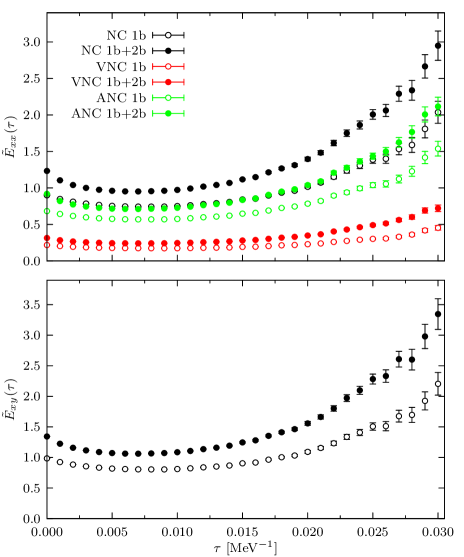
Figure 2: (Color online) Euclidean neutral-weak transverse (top panel) and interference (lower panel) response functions ($\alpha\beta=xx$ and $xy$ in the notation of Ref. Shen et al. (2012)) of ¹²C at $q=570$ MeV. See text for further explanations.

The VNC consists of a linear combination of the isoscalar and isovector components of the electromagnetic current, weighted respectively by the factors $-2\,\sin^{2}\theta_{W}$ and $(1-2\,\sin^{2}\theta_{W})$ with $\theta_{W}$ being the Weinberg angle. The excess transverse strength induced by two-body terms in the VNC is consistent with that found in the transverse electromagnetic response, and is confirmed by experiment as Fig. 1 demonstrates. The two-body enhancement in the (ANC-ANC) contribution of $E_{xx}(q,\tau)$ is substantial at these relatively large $q$’s. It decreases significantly (for $\tau\gtrsim 0.01$ MeV^-1) as $q$ is reduced Lovato et al. (2015), consistently with what is found in calculations of low $q$ charge-changing weak transitions to specific low-lying states, such as the $\beta$-decays and electron and muon captures studied in Refs. Schiavilla and Wiringa (2002); Marcucci et al. (2011), where it amounts to a few percent. In principle, the enhancement in the quasi-elastic region could be measured in parity-violating inclusive $(\vec{e},e^{\prime})$ scattering at backward angles. However, the smallness of the factor $(1-4\,\sin^{2}\theta_{W})$, to which the relevant (VEM-ANC) interference response function is proportional, makes experiments of this type extremely difficult.

In order to obtain more detailed information on the energy dependence of the $R_{\alpha\beta}(q,\omega)$ response, we employ the maximum entropy (MaxEnt) method to invert $E_{\alpha\beta}(q,\tau)$. We describe the method here very briefly, several standard references are available Bryan (1990); Jarrell and Gubernatis (1996). The numerical inversion of a Laplace transform $E_{\alpha\beta}(q,\tau)$ with its associated statistical errors is a notoriously ill-posed problem. The fact that we are interested in the (smooth) response around the quasi-elastic peak rather than isolated peaks makes it somewhat more practical. The MaxEnt method is based on Bayesian statistical inference: the “most probable” response function is the one that maximizes the posterior probability Pr$[R|\overline{E}\,]$, i.e., the conditional probability of $R$ given $\overline{E}$. Bayes theorem states that the posterior probability is proportional to the product ${\rm Pr}[\,\overline{E}|R\,]\times{\rm Pr}[R\,]$, where Pr$[\,\overline{E}|R\,]$ is the likelihood function and Pr$[R\,]$ is the prior probability. Arguments based on the central limit theorem show that the asymptotic limit of the likelihood function is given by Pr$[\,\overline{E}|R\,]\propto{\rm exp}(-\chi^{2}/2)$ with $\chi^{2}$ defined as follows. Let $N_{\tau}$ and $N_{\omega}$ be the numbers of grid points in the variables $\tau$ and $\omega$, respectively. Then the Laplace transform in Eq. (2) reads (the $q$-dependence and subscripts $\alpha\beta$ of $E_{\alpha\beta}(q,\tau)$ and $R_{\alpha\beta}(q,\tau)$ are suppressed for simplicity hereafter)

$$E_{i}=\sum_{j=1}^{N_{\omega}}K_{ij}\,R_{j}\ ,$$ (4)

where $K_{ij}={\rm exp}(-\tau_{i}\,\omega_{j})$ and $R_{j}=\Delta\omega_{j}\,R(\omega_{j})$, and the $\chi^{2}$ follows from

$$\chi^{2}=\sum_{i,j=1}^{N_{\tau}}\left(\,\overline{E}_{i}-E_{i}\right)\left(C^{-1}\right)_{ij}\left(\,\overline{E}_{j}-E_{j}\right)\ ,$$ (5)

where the $E_{i}$ are obtained from Eq. (4), the $\overline{E}_{i}$ are the GFMC calculated values, and $C$ is the covariance matrix. Therefore, maximizing the likelihood function reduces to finding a set of $R_{i}$ values that minimizes the $\chi^{2}$. The GFMC errors on $\overline{E}_{i}$ are strongly correlated in $\tau$, as individual steps involve only small spatial distances and evolutions of the spin-isospin amplitudes. It is therefore of paramount importance to estimate the covariance matrix $C$.

Limiting ourselves only to the $\chi^{2}$ minimization would implicitly be making the assumption that the prior probability is either unimportant or unknown. However, since the response function is positive definite and normalizable, it can be interpreted as yet another probability function. The principle of maximum entropy states that the values of a probability function are to be assigned by maximizing the entropy

$$S=\sum_{i=1}^{N_{\omega}}\Big{[}R(\omega_{i})-M(\omega_{i})-R(\omega_{i})\ln[R(\omega_{i})/M(\omega_{i})]\Big{]}\Delta\omega_{i}\,,$$ (6)

where the positive definite function $M(\omega)$ is the default model. It is worthwhile mentioning that the above expression is applicable even when $R(\omega)$ and $M(\omega)$ have different normalizations. The entropy measures how much the response function differs from the model. It vanishes when $R(\omega)=M(\omega)$, and is negative when $R(\omega)\neq M(\omega)$. The maximum entropy method adds to the simple $\chi^{2}$ minimization the use of the prior information that the response function can be interpreted as a probability distribution function. We employ historic maximum entropy by minimizing $\alpha\,S-\chi^{2}/2$ with the parameter $\alpha$ adjusted to make the $\chi^{2}$ equal to one. While more refined methods relying on Bayes statistical inference have been developed, we found historic maximum entropy to be simple to implement and adequate for our purposes.

As a first case we consider the electromagnetic response of ⁴He. We generated a set of $N_{E}\simeq 2500$ GFMC estimates of the Euclidean response functions, obtained from independent imaginary-time propagations on a grid of $\tau$ points uniformly distributed between 0 to 0.05 MeV^-1 with $\Delta\tau=0.0005$ MeV^-1. Let $E^{(n)}_{i}=E^{(n)}(\tau_{i})$ be the Euclidean response function corresponding to the $n^{\rm th}$ GFMC propagation. The average Euclidean response function and covariance matrix elements are given by

$$\overline{E}_{i} =\frac{1}{N_{E}}\sum_{n=1}^{N_{E}}E^{(n)}_{i}\ ,$$ (7)

$$C_{ij} =\frac{1}{N_{E}(N_{E}-1)}\sum_{n=1}^{N_{E}}E^{(n)}\!\!\left[\overline{E}_{i}-E_{i}^{(n)}\right]\!\!\left[\overline{E}_{j}-E_{j}^{(n)}\right]\,.$$ (8)

In general, the covariance matrix is non-diagonal because of correlations between different $\tau_{i}$, and the full expression for the $\chi^{2}$ in Eq. (5) has been used.

The ⁴He longitudinal and transverse response functions (at $q=600$ MeV), obtained from inversion of $E_{L}(q,\tau)$ and $E_{T}(q,\tau)$, are shown in Fig. 3. The inversions are, to a very large degree, insensitive to the choice of default model response Lovato et al. (2015). Results obtained with one-body only (dashed line) and (one+two)-body (solid line) currents are compared with experimental world data Carlson et al. (2002) (empty circles). There is excellent agreement between the full theory and experiment. Two-body currents significantly enhance the transverse response function, not only in the dip region, but also in the quasi-elastic peak and threshold regions, providing the missing strength needed to reproduce the experimental results. The band in Fig. 3 provides an estimate for the dependence of the full results on the adopted default model, either a flat $M(\omega)$ or a gaussian one Lovato et al. (2015). The model dependence is quite small.

On the basis of the present ⁴He and ¹²C calculations, a consistent picture of the electroweak response of nuclei emerges, in which two-body terms in the nuclear electroweak current are seen to produce significant excess transverse strength from threshold to the dip region and beyond. Such a picture is at variance with the conventional one of inclusive quasi-elastic scattering, in which single-nucleon knockout is expected to be the dominant process in this regime. With the exception of the leading relativistic corrections contained in the nuclear electroweak currents (see Ref. Shen et al. (2012)), the present calculations are based on a nonrelativistic approach. Naive kinematical considerations would lead one to expect the quasi-elastic peak position in Fig. 3 to be at $q^{2}/(2\,m)+\Delta E\simeq 211$ MeV for $q=600$ MeV—we take $\Delta E\simeq 20$ MeV to be the separation energy of ⁴He into a 3+1 cluster. The calculated response functions appear to peak at lower $\omega$, in fact close to $\omega_{\rm qe}+\Delta E\simeq 195$ MeV. The width of the quasi-elastic peak is also seen to be correctly reproduced—the nonrelativistic Fermi gas fails to predict this quantity at momentum transfers $q\sim 600$ MeV as in Fig. 3. Thus, even at these relatively high momentum and energy transfers, the nonrelativistic dynamical framework adopted here may be more robust than comparisons between nonrelativistic and relativistic Fermi gas models would lead one to conclude Pace et al. (2003).

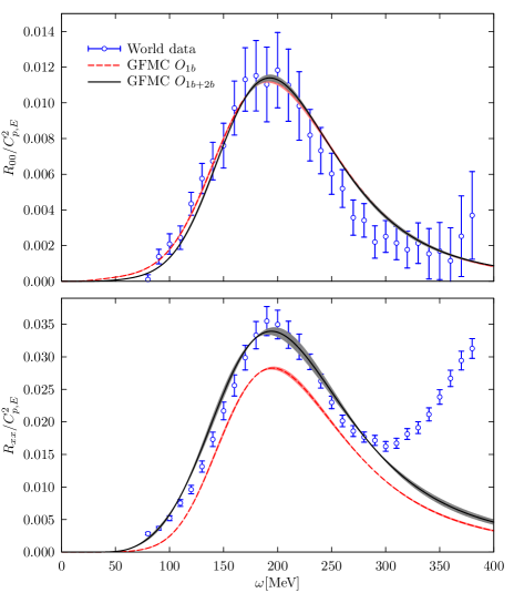
Figure 3: (Color online) Electromagnetic longitudinal (top panel) and transverse (lower panel) response functions of ⁴He at $q=600$ MeV. Experimental data are from Ref. Carlson et al. (2002).

A direct evaluation of the ¹²C response functions via these same methods would require about 100 million core hours. We are examining improved methods including the use of correlated sampling that could improve the efficiency of this inversion. We are also exploring methods to extend these results to larger nuclei.