The Efficiency of Stellar Reionization:
Effects of Rotation, Metallicity, and Initial Mass Function

Abstract

We compute the production rate of photons in the ionizing Lyman continua (LyC) of H I ($\lambda\leq 912$ Å), He I ($\lambda\leq 504$ Å), and He II ($\lambda\leq 228$ Å) using recent stellar evolutionary tracks coupled to a grid of non-LTE, line-blanketed WM-basic model atmospheres. The median LyC production efficiency is $Q_{\rm LyC}=(6\pm 2)\times 10^{60}$ LyC photons per $M_{\odot}$ of star formation (range $[3.1-9.4]\times 10^{60}$) corresponding to a revised calibration of $10^{53.3\pm 0.2}$ photons s^-1 per $M_{\odot}$ yr^-1. Efficiencies in the helium continua are $Q_{\rm HeI}\approx 10^{60}$ photons $M_{\odot}^{-1}$ and $Q_{\rm HeII}\approx 10^{56}$ photons $M_{\odot}^{-1}$ at solar metallicity and larger at low metallicity. The critical star formation rate needed to maintain reionization against recombinations at $z\approx 7$ is $\dot{\rho}_{\rm SFR}=(0.012\;M_{\odot}\;{\rm yr}^{-1}\;{\rm Mpc}^{-3})[(1+z)/8]^{3}(C_{\rm H}/3)(0.2/f_{\rm esc})$ for fiducial values of IGM clumping factor $C_{H}\approx 3$ and LyC escape fraction $f_{\rm esc}\approx 0.2$. The boost in LyC production efficiency is an important ingredient, together with metallicity, $C_{H}$, and $f_{\rm esc}$, in assessing whether IGM reionization was complete by $z\approx 7$. Monte-Carlo sampled spectra of coeval starbursts during the first 5 Myr have intrinsic flux ratios of $F(1500)/F(900)\approx 0.4-0.5$ and $F(912^{-})/F(912^{+})\approx 0.4-0.7$ in the far-UV (1500 Å), the LyC (900 Å), and at the Lyman edge (912 Å). These ratios can be used to calibrate the LyC escape fractions in starbursts.

1. INTRODUCTION

Photons in the Lyman continuum (LyC) of hydrogen (energies $E\geq 13.60$ eV and wavelengths $\lambda\leq 911.753$ Å) play a crucial role in theoretical and observational studies of H II regions, active galactic nuclei (AGN), starburst galaxies, and ionization of the interstellar medium (ISM) and intergalactic medium (IGM). The dominant sources of ionizing photons in the ISM are O-type stars (Spitzer 1978), while the metagalactic ionizing background arises from both O-type stars and AGN (Haardt & Madau 2001, 2012; Shull et al. 1999). Photoionization by hot stars is also the likely process governing the H I epoch of reionization at redshifts $z\approx 7$) ending the transition from the “dark ages” following cosmological recombination at $z\approx 1100$ through “first light” at $z\approx 30-50$.

The redshift frontier for detection of early galaxies is now at $z\approx 10$ using the Lyman-break flux dropout technique with the Wide-Field Camera-3 (WFC3) aboard the Hubble Space Telescope (Bouwens et al. 2011; Bradley et al. 2012; Ellis et al. 2013; Robertson et al. 2013; Schmidt et al. 2014). These distant galaxies allow us to explore stellar populations during the epoch ($z=7-10$) when reionization was well underway. The critical star formation rate (SFR) density, $\dot{\rho}_{\rm SFR}\approx 0.02\ \,M_{\odot}~{}{\rm yr}^{-1}~{}{\rm Mpc}^{-3}$ at $z\approx 7$, defines the photoionization rate needed to balance IGM recombinations (Madau et al. 1999; Shull et al. 2012). However, estimating the number of ionizing photons in the radiation field requires calibrating the O-star production rates and extrapolating the galaxy luminosity function well below the observed populations (Trenti et al. 2011; Finkelstein et al. 2012; Robertson et al. 2013). The main parameters in $\dot{\rho}_{\rm SFR}$ include the net production rate and escape fraction of Lyman continuum (LyC) photons by hot stars and structural properties of the ISM and IGM. Current estimates suggest that galaxies should be able to complete reionization by $z\approx 7$, although the details depend on LyC production efficiencies.

The LyC production efficiency (ionizing photons per solar mass of star formation) is a standard parameter in cosmological simulations of galaxy formation and IGM reionization. Historically, many groups have assumed a constant rate of $10^{53.1}$ photons s^-1 per $M_{\odot}$ yr^-1. The current calculation explores the dependences of this parameter on metallicity, initial mass function (IMF), and stellar rotation. Because of the importance of O-star ionizing photon production (Vacca et al. 1996; Schaerer & Vacca 1998; Oey et al. 2000; Kewley et al. 2001; Smith et al. 2002; Sternberg et al. 2003; Martins et al. 2005; Leitherer et al. 2010) to the study of starburst galaxies and the epoch of reionization, there is a need for more accurate calculations. This can now be done, with improvements in stellar atmospheres modeling, including three-dimensional expanding atmospheres, non-LTE radiative transfer, populations of the hydrogen and helium ground states, and an increased number of spectral lines in the line blanketing and force modeling of stellar winds. For stellar populations, the LyC production rates depend on the initial mass function (IMF), evolutionary tracks, and model atmospheres, all of which may change at low metallicity and with rapid stellar rotation (Schaerer 2003; Ekström et al. 2012; Georgy et al. 2013). Some of the recent tracks also include the effects of rotation on stellar structure and evolution at different metallicities.

In this paper, we compute the production efficiency (LyC photons per solar mass of star formation). We use new evolutionary tracks of various metallicities, with and without rotation, together with ionizing spectra from model atmospheres. We find the production rates of photons in the ionizing continua of H I, He I, and He II by integrating over a grid of stellar tracks coupled to non-LTE, line-blanketed stellar atmospheres using the WM-basic code (Pauldrach et al. 2001; Puls et al. 2005) with a consistent metallicity. Section 2 describes our procedure for deriving the stellar LyC from evolutionary tracks and consistent model atmospheres. Section 3 explains our methods for generating a grid of atmosphere models overlaid on evolutionary tracks of solar and sub-solar metallicities, with and without rotation. In Section 4 we present and analyze results for the ionizing photon luminosities and lifetime-integrated LyC production efficiencies, for both the hydrogen LyC as well as the continua of He I and He II (the latter is especially sensitive to metallicity and rotation). In Section 4.3, we apply the new LyC efficiencies to IGM reionization and critical SFR at $z\approx 7$. Section 5 provides a summary and a discussion of future directions in the field.

2. COMPUTING THE STELLAR LYMAN CONTINUUM

Our LyC calculation relies on coupling a full grid of stellar evolutionary tracks with model atmospheres. Although it would be desirable to explore a wider range of other parameters (mass-loss rates, clumpy and porous winds, and binaries) there are no complete evolutionary tracks for such parameters. Thus, we rely on stellar grids from the Geneva group (Schaerer 2003; Ekström et al.  2012; Georgy et al.  2013). Our computational procedure begins with these evolutionary tracks, which provide the key stellar parameters: effective temperature ($T_{\rm eff}$), surface gravity ($\log g$), mass ($M$), and radius ($R_{*}$). From atomic data and stellar opacities, we run new model atmospheres to compute the spectral energy distribution (SED) with astrophysical flux ($F_{\lambda}$) in units of erg cm^-2 s^-1 Å^-1. We derive the integrated ionizing photon fluxes, $q_{i}$ (phot cm^-2 s^-1), from the star’s surface for the H I, He I, and He II continua by integrating the modeled spectra over wavelengths $\lambda\leq\lambda_{\rm lim}^{(i)}$,

$$q_{i}=\int_{0}^{\lambda^{(i)}_{\rm lim}}\frac{\pi\lambda F_{\lambda}}{hc}\,d\lambda\;.$$ (1)

Here, $hc/\lambda$ is photon energy and $\lambda_{\rm lim}^{(i)}$ correspond to the H I, He I, and He II continuum edges at $\lambda_{\rm lim}=911.753$ Å, 504.259 Å, and 227.838 Å for indices $i=$ 0, 1, and 2 respectively.

We combine the evolutionary tracks and grid of model atmospheres consistently to obtain an updated grid ($T_{\rm eff}$, $\log g$) where each point contains information on photon fluxes instead of the entire synthetic spectrum. The star’s ionizing photon luminosities $Q_{i}=4\pi R_{*}^{2}q_{i}$ (photons s^-1) are found from the star’s surface area at each point along the evolutionary track for a star of radius $R_{*}(t)$ and initial mass $M$. The lifetime-integrated values of $Q_{0}$, $Q_{1}$, and $Q_{2}$ are then derived for the H I, He I, and He II continua. Thus, $Q_{0}^{\rm(tot)}(m)$ gives the total number of ionizing (LyC) photons produced over a massive star’s life, where $m=M/M_{\odot}$ is in solar-mass units. For O-type stars in the range $25\leq m\leq 100$, typical values are $Q_{0}^{\rm(tot)}\approx(1-10)\times 10^{63}$ photons. These photon production numbers can then be summed over a stellar IMF using one of the common distributions (Salpeter 1955; Kroupa 2001; Chabrier 2003) to determine the number of ionizing photons produced by a stellar population. A similar grid of WM-basic model atmospheres at solar metallicity was computed by Sternberg et al. (2003). Our calculations are done with updated stellar parameters appropriate for the new evolutionary tracks.

Reionization models and cosmological simulations require a relationship between SFR and LyC production rate. This calibration is often expressed as the standard ratio (Madau et al. 1999) of $10^{53.1}$ photons s^-1 per $M_{\odot}$ yr^-1. We adopt an average LyC production rate over the age of an OB starburst. Without great loss of accuracy, one can simply cancel the time units ($3.1556\times 10^{7}$ s/yr) and quote the equivalent standard ratio as $Q_{\rm LyC}=4\times 10^{60}$ LyC photons per solar mass of star formation. In this paper, we follow the convention used by Shull et al. (2012) in their reionization models, where they define the ratio

$$Q_{\rm LyC}=\frac{\int_{m_{min}}^{m_{max}}Q_{i}^{\rm(tot)}(m)\xi(m)\,\mathrm{d}m}{\int_{m_{min}}^{m_{max}}\xi(m)m\,\mathrm{d}m}\;.$$ (2)

Here, $\xi(m)$ represents the differential distribution of stars per unit mass (not per $\log m$ as sometimes defined), and the integration is between mass limits $m_{\rm min}$ and $m_{\rm max}$. For convenient units, we express $Q_{\rm LyC}$ in $10^{63}$ photons per $M_{\odot}$ of star formation. For a range of metallicities, $0.1\leq(Z/Z_{\odot})\leq 1$, older model atmospheres, and a Salpeter IMF, Shull et al. (2012) found that $Q_{\rm LyC}\approx 0.0024-0.0038$ ($\times 10^{63}$ photons per $M_{\odot}$). Below, we update this calibration factor using new stellar data on LyC production and exploring the effects of lower metallicity and increased rotation.

3. COMPUTATIONAL METHODS FOR TRACKS AND ATMOSPHERES

The earliest stellar evolutionary tracks included only a small amount of stellar physics that was computationally allowed at the time. These models solved the equations of stellar structure with little treatment of more advanced physics. Some of the first standard evolutionary tracks came from the Geneva group in the early 1990’s (Schaller et al. 1992; Schaerer et al. 1993a,b; Charbonnel et al. 1993). After observations suggested higher mass loss rates for massive stars, additional set of tracks were produced (Meynet et al. 1994; Fagotto et al. 1994a,b). The next major advance was to add the effects of stellar rotation. Although the early efforts were productive, they only described some effects of rotation and did not extend to $M<9\;M_{\odot}$ (Meynet & Maeder 2000).

For the past two decades, the most widely used stellar evolutionary tracks were those of Schaller et al. (1992). The most recent tracks (see Figure 1) computed at solar metallicity (Ekström et al. 2012) and sub-solar metallicity (Georgy et al. 2013) are expected to become the new standard in the field. These models surpass previous evolutionary tracks with their treatment of mass loss from the stellar wind, more accurate nuclear burning rates, and the addition of stellar rotation. Advances in helioseismology and other stellar observations have improved our understanding of the interior properties of rotating stars. From these data, Ekström et al. (2012) created evolutionary tracks and isochrones for a wide mass range of rotating and corresponding non-rotating stars. These models can be used to create an initial picture of rotating stellar evolution. One of the most important differences with rotation is mixing caused by meridional circulation, which continuously provides new fuel to burn in the core and increases the lifetime of a star.

Figure 1.— New rotating tracks (Ekström et al. 2012; Georgy et al. 2013). Tracks computed at solar metallicity (top) and sub-solar metallicity (bottom). Note different post main sequence populations at low metallicity, with fewer “blue-loop” excursions and fewer WR stars.

Improvements in the quality of model atmospheres include non-LTE treatment of the radiation field, wind and line blanketing, and increased code efficiency. The first upgrades involved an efficient method for approximating the radiation pressure due to spectral lines. The CAK model (Castor, Abbott & Klein 1975) averaged the radiative force over all lines instead of treating them separately. This increase in radiative force led to higher mass loss rates. Even with this advance, atmosphere models were restricted to local thermodynamic equilibrium (LTE), requiring a blackbody radiation field and Boltzmann level populations. Pauldrach et al. (1986) upgraded the CAK model by neglecting the radial-streaming approximation for photons that drive the stellar wind. Rotational effects were found to be negligible for rotational velocities $v_{\rm rot}<200$ km s^-1.

Advances in model atmospheres have been more consistent than advances in evolutionary tracks, primarily because of the availability of fast computers. The most efficient codes still use a modified version of the CAK method to compute line forces, because it is fast and its approximations provide efficiency. Perhaps the most important improvement is the extension of the models into the non-LTE regime, allowing the radiation field to deviate from Planckian and level populations from Boltzmann. Other advances include solving the radiative transfer equations in co-moving coordinates, moving away from plane-parallel models, and increasing the accuracy of atomic data. With these recent improvements, a model atmosphere can now be computed in less than ten minutes, allowing thousands of models to be computed over the course of the project and providing accurate time resolution for the evolution of stellar spectra. A few of the most prominent atmosphere codes are: TLUSTY (Lanz & Hubeny 2003, 2007), FASTWIND (Puls et al. 2005), CMFGEN (Hillier & Miller 1998), and WM-basic (Pauldrach et al. 2001).

For our model atmospheres we chose the WM-basic code primarily because of its hydrodynamic solution of spherically expanding atmospheres with line blanketing and non-LTE radiative transfer and its treatment of the continuum and lines in the ionizing EUV. This code is also a standard for theoretical atmosphere modeling in the population synthesis code Starburst99 (Leitherer et al. 1999, 2014). An extensive discussion of hot-star atmosphere codes appears in papers by Martins et al. (2005) and Leitherer et al. (2014). A comparison of the ability of these codes to fit stellar lines, effective temperatures, and surface gravities was made by Puls (2008) and Massey et al. (2013). In Figure 2 we show the results of WM-basic and CMFGEN for three cases with $T_{\rm eff}\approx$ 30kK, 40kK, and 50kK. The agreement is reasonably good, given the different model input parameters required to arrive at similar effective temperatures, but slightly different $\log g$ values.

Figure 2.— Overlaid comparison of model atmospheres at effective temperatures $T_{\rm eff}\approx 30$ kK, 40 kK, and 50 kK, computed using the WM-basic and CMFGEN code with emergent fluxes $F_{\lambda}$ in units $10^{11}$ erg cm^-2 s^-1 Å^-1. Because of slight differences in mass-loss rates and required input parameters for the stellar models, we are unable to precisely match effective temperatures ($T_{\rm eff}$) and surface gravities ($\log g$). The WM-basic model is shown in black and the CMFGEN model in red.

3.1. Evolutionary Tracks

We use evolutionary tracks from Schaller et al. (1992), Ekström et al. (2012), and Georgy et al. (2013). These models include fixed prescriptions for stellar mass loss during late stages of evolution, and they provide a convenient means of assessing the effects of metallicity and rotation. It would be useful to assess the dependence of LyC production rates on alternative prescriptions for mass loss, particularly during late stages of massive-star evolution. However, at the current time, we are constrained to using the available evolutionary tracks. The field of massive-star evolution continues to present challenges to the correct implementation of these effects (Vink 2014; Martins 2014; Hirschi 2014) as well as those of binaries and stellar mergers (Eldridge et al. 2008; de Mink et al. 2013, 2014). Populations of very massive stars (150–300 $M_{\odot}$) may exist in the Arches cluster (Figer et al. 2002; Crowther et al. 2010), in the dense R136 star cluster in 30 Doradus, and in the Galactic cluster NGC 3603 (Crowther et al. 2010; Martins 2014). Figer (2005) used the Arches cluster to set an upper mass limit of 150 $M_{\odot}$, owing to an absence of stars with initial masses $\geq 130$ $M_{\odot}$. These mass estimates are subject to uncertainties in stellar luminosity arising from cluster distance, extinction laws, and effective temperatures. As summarized in recent reviews (Vink 2014; Martins 2014), there are several stars that could have masses between 100-200 $M_{\odot}$. Such stars could provide additional sources of LyC by extending the IMF above the last grid point on the evolutionary tracks. On the other hand, the most massive stars in dense clusters are deeply embedded in star-forming clouds, and their LyC may not escape until after these regions clear of gas and dust.

For the current calculation, we truncate all IMFs at a maximum mass of 120 $M_{\odot}$, and we use the LyC production rates to describe massive star formation regions and reionization of the IGM. The tracks are computed at five different metallicities, of which we consider three for non-rotating stars. In the Hertzsprung-Russell (H-R) diagram stellar evolution defines the basic parameters ($M_{*}$, $L_{*}$, $T_{\rm eff}$, $\log g$) which are related by self-consistency. For example, surface gravity $g=GM_{*}/R_{*}^{2}$ depends on stellar mass $M_{*}$ and radius $R_{*}$, and stellar luminosity $L_{*}=4\pi R_{*}^{2}\sigma T_{\rm eff}^{4}$ depends on effective temperature $T_{\rm eff}$ and $R_{*}$. The ionizing fluxes are sensitive primarily to $T_{\rm eff}$. We use different evolutionary tracks to investigate how different stellar physics can affect the production of LyC photons. The first set of tracks are from Schaller et al. (1992), a past standard for non-rotating stars with sub-solar, solar, and super-solar metallicities, $Z=0.004$, 0.02 and 0.04, respectively, by mass. The second set of tracks comes from the same group (Ekström et al. 2012) with a mass range extended to $0.8$ $M_{\odot}$ $\leq$ $m$ $\leq$ $120$ $M_{\odot}$  and finer mass resolution. One essential advance is their treatment of rotation. We use two sets of tracks with metallicities $Z=0.004$ and $Z=0.014$, each computed with an initial rotation of 40% of the critical rotation speed. We also consider their tracks without rotation. Since the Schaller et al. (1992) work, the accepted value for the solar metallicity has decreased to either $Z_{\odot}=0.014$ (Asplund et al. 2009) or $Z_{\odot}=0.0153$ (Caffau et al. 2011). Ekström et al. (2012) calculated both rotating and non-rotating tracks at solar metallicity ($Z=0.014$), while Georgy et al. (2013) computed both rotating and non-rotating tracks at sub-solar metallicity ($Z=0.002$). The Geneva group has not yet provided new tracks with super-solar metallicity.

3.2. Model Atmospheres

After compiling the evolutionary tracks, we produce model spectra at each time step along the track. We use the atmosphere code WM-basic because of its efficiency and ability to generate accurate spectra, including lines in the UV and EUV. The code requires only a few basic parameters ($T_{\rm eff}$, $\log g$, $R_{*}$, abundances) to compute a model. For each set of tracks we compute a grid of atmospheres in the $(T_{\rm eff},\log g)$ plane and follow the evolution of the ionizing spectra of a star through time. We use the flux distributions to find the total LyC flux and integrate to calculate the ionizing photon production for each initial mass. An atmosphere model can be completed in 10-15 minutes on a desktop computer. Over the course of our project, we ran hundreds of atmosphere models to achieve accurate time resolution along evolutionary tracks. One full grid of models for a set of evolutionary tracks contains around 100 atmosphere models.

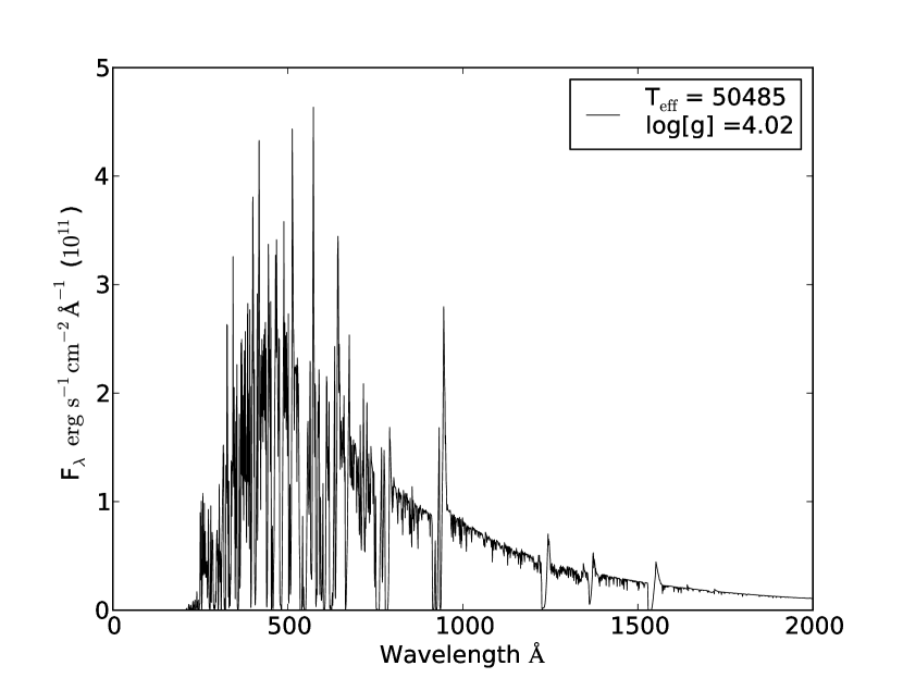
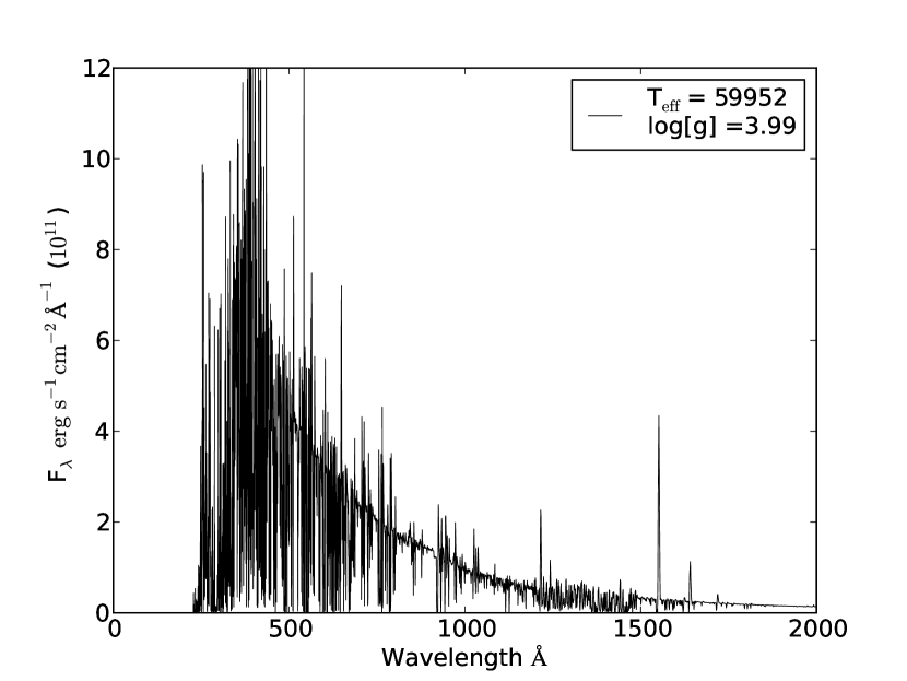
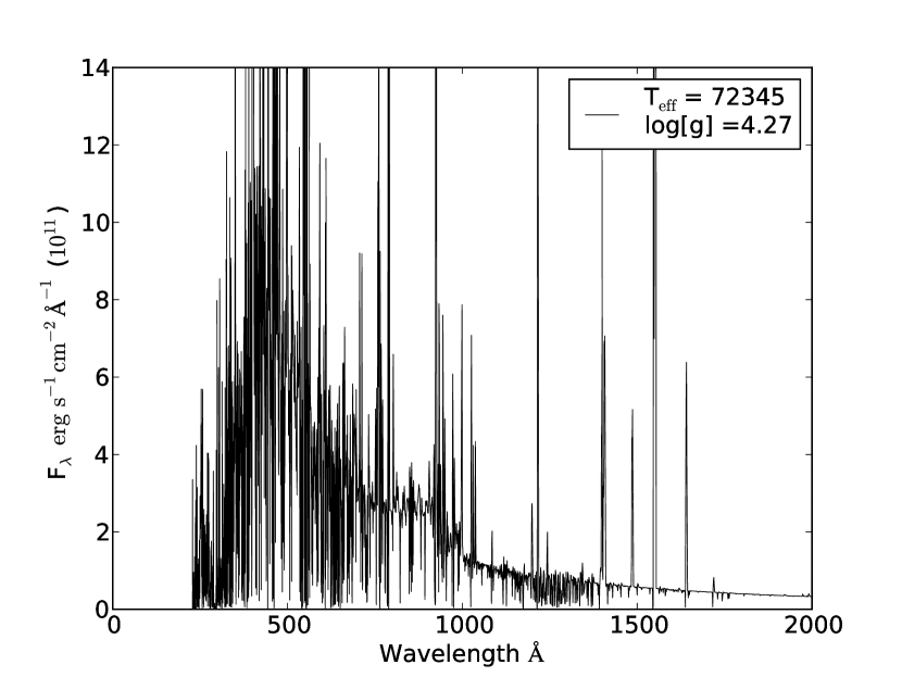
Figure 3.— Six model atmospheres computed using the WM-basic atmosphere code and taken from the Ekström et al. (2012) grid of rotating tracks at solar metallicity ($Z=0.014$). Models are shown in 10kK intervals in $T_{\rm eff}$; we include 45kK because of the rapid change in strength of the H and He edges in that temperature range. Models are all for O-type stars near the main sequence.

The process of model atmosphere calculation comes in three different pieces: the hydrodynamics, calculation of the occupation numbers and radiation field, and production of the synthetic spectrum. The hydrodynamics section is where the initial parameters are input, most importantly $T_{\rm eff}$, $\log g$, and $R_{*}$. From these, the code finds the mass, luminosity, and other basic data. The next input are the abundances of elements between H and Zn, with three options: solar metallicity, solar metallicity while defining the H and He abundances, and custom-defined abundances. Because the default “solar” abundances programmed into the code were outdated, we used the recent standard of $Z_{\odot}=0.014$ by mass (Asplund et al. 2009). The code requires input of the metal abundances relative to solar, which we re-examine after a model is run. In its normalization procedure, one can alter the abundances. The resulting values may differ from the input values, but generally by only a few percent. Once the input file is written, the model can be run using the graphical user interface.

For the radiation force on the atmosphere and wind, we use three line-force parameters ($k$, $\alpha$, $\delta$) in the CAK method. This method approximates the sum of a large number of spectral lines, with temperature assumed to be constant throughout the atmosphere to increase the efficiency. The hydrodynamics calculation is iterated two more times. The first time, the temperature gradient is computed using the continuum opacities. In the last iteration the temperature is computed including the line opacities. The code then computes the photon energy, occupation numbers, and radiation field in the NLTE regime. This step provides the radiation field, final temperature structure, information about opacities, and occupation numbers for the various elements using detailed atomic models. The final step in the calculation provides the synthetic spectrum. Figure 3 illustrates the continuum shapes from models with $T_{\rm eff}$ ranging from 31,800 K to 72,300 K, particularly the contributions of emission lines, the depth of the Lyman edge, $F(912^{-})/F(912^{+})$, and the ratio, $F(1500)/F(910)$, of fluxes at 1500 Å and 900 Å. The latter two ratios have been used to calibrate the escape fraction ($f_{\rm esc}$) of LyC radiation. This observational technique was introduced by Steidel et al. (2001) and employed by Inoue et al. (2005), Shapley et al. (2006), and Mostardi et al. (2013) to estimate $f_{\rm esc}$ in star-forming galaxies at $z=2.85-3.27$. In their method, the observed flux-density ratio, $[F(1500)/F(910)]_{\rm obs}$, is compared to estimates of the intrinsic ratios determined from the models. We return to this issue in Section 4.5, where we discuss the intrinsic values, $[F(1500)/F(910)]_{\rm int}\approx 0.4-0.7$ found in our modeled composite spectra of OB associations with coeval starbursts.

In the models of Figure 3 with $T_{\rm eff}<50,000$ K, the absorption edge at the Lyman limit is clearly visible at $\lambda=912$ Å. Figure 4 shows two models at $T_{\rm eff}\approx 41,000$ K with metallicities $Z=0.014$ (solar) and $0.004$ (sub-solar) by mass. Each has an intrinsic Lyman edge resulting from the non-LTE level population of the ground state of H I. Differences in metallicity have a minor effect on the depth of the edge, which arises primarily from surface abundances and heating. However, the EUV fluxes are affected by emission lines in the stellar wind, which increase in strength at higher metallicity (left panel of Figure 4).

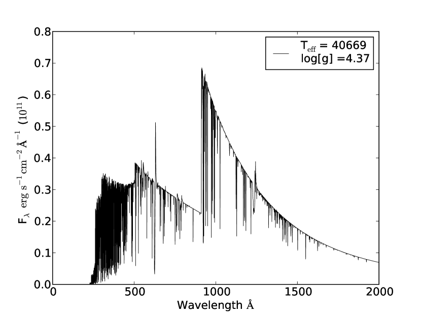
Figure 4.— Two model atmospheres with $T_{\rm eff}\approx 41$kK, computed using the WM-basic atmosphere code showing metallicity effects on the strength of the Lyman edge at 912 Å and emission lines from the stellar wind. Left: Solar metallicity model ($Z=0.014$) has a 57% drop in flux at the continuum edge and substantial metal emission lines in the EUV band (300-900 Å). Right: Sub-solar metallicity model ($Z=0.004$) has a 68% continuum drop and many fewer emission lines.

3.3. Grid of Atmosphere Models for Evolutionary Tracks

In order to find the integrated LyC photon production over an O-star’s lifetime, we set up a grid of spectra in the ($T_{\rm eff},\log g$) plane defined by the initial mass of the evolutionary track (Figure 5). We distribute the grid points evenly along points of equal time. Because the grid has a higher density where the stars spend more time, we obtain a higher accuracy of photon fluxes over the stellar lifetime and improve the accuracy of the integrated photon fluxes. As the most massive stars shed their atmospheres in late stages of evolution (Figure 6), they move quickly through “blue loops” and into the Wolf-Rayet (WR) phase. Although the most massive stars spend only a short time in these regions of the H-R diagram, their LyC production rate is high. Therefore, we compute extra atmosphere models and ensure that we place sufficient grid points during these late stages to capture the ionizing radiation.

The WR stars deserve further discussion as the evolutionary descendants of massive stars ($M\geq 25~{}M_{\odot}$) characterized observationally by broad emission lines, strong stellar winds, and mass-loss rates up to $10^{-5}~{}M_{\odot}~{}{\rm yr}^{-1}$ (Maeder & Conti 1994; Crowther 2007; Massey 2013). Both luminous ($L>10^{5}\,L_{\odot}$) and hot (25,000–100,000 K), WR stars can contribute substantially to the LyC production of a stellar population, particularly in the He I and He II continua. However, the canonical estimate that WR stars are 10% of the massive-star population is based on little more than the He-burning lifetimes of stars with $M\geq 25~{}M_{\odot}$ estimated from uncertain evolutionary tracks. Because O-star mass-loss rates depend on metallicity, it should be easier to become a WR star at high metallicity. This expectation appears to agree with observations, which show fewer WRs at low metallicity in Local Group galaxies (Maeder et al. 1980; Hamann et al. 2006; Neugent et al. 2012; Massey et al. 2014). However, the progenitor masses and details of post-main-sequence stellar evolution that lead to the various (WC, WN, WO) sub-classes are still poorly understood. Recent surveys of WN and WC stars in the Galaxy, LMC, and M31 (Sander et al. 2012; Sander et al. 2014; Hainich et al. 2014) suggest that WN progenitors originate from initial masses between 20–60 $M_{\odot}$. The ratios of WR stars to O stars (and of WN and WC subtypes) are frequently used as tests of massive-star evolutionary models. Owing to uncertainties in distance and reddening and selection biases in detecting WR stars relative to O-type stars, astronomers probably cannot measure the Galactic (WR/O) ratio to better than 50% (Massey et al. 1995).

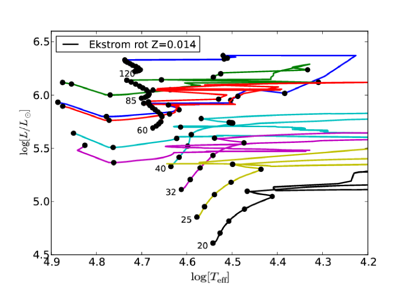
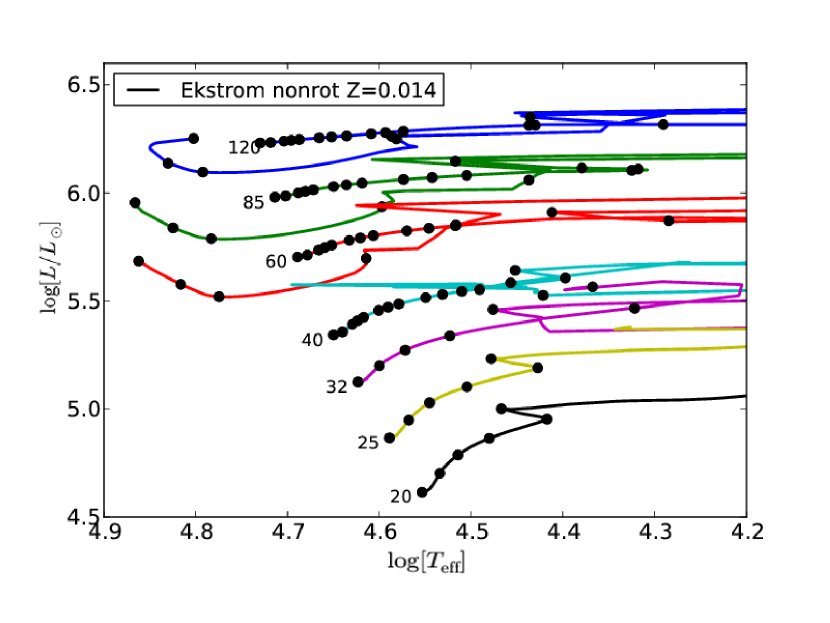
Figure 5.— Top: Evolutionary tracks (Ekström et al. 2012) at solar metallicity computed with rotation and labeled by initial mass (in $M_{\odot}$). Bottom: Corresponding non-rotating tracks. Points along tracks show values of $T_{\rm eff}$ and $L$ at which model atmospheres were computed.

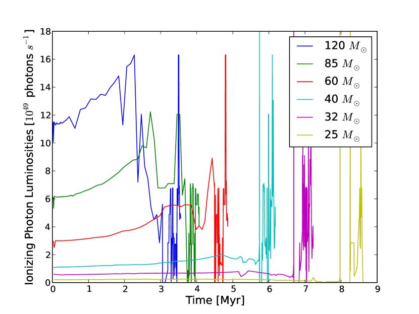
Figure 6.— The LyC photon luminosities, $Q_{0}(t)$, versus time for Ekström et al. (2012) rotating evolutionary tracks with $Z=0.014$. Each line shows a track with different initial mass from 120 $M_{\odot}$ to 25 $M_{\odot}$ (top to bottom). Rapid spikes show “blue loops” and Wolf-Rayet phase at the end of the star’s lifetime. Although WR stars take up a small fraction of the lifetime, we have ensured that sufficient model atmospheres are placed to capture the LyC produced in these late phases of evolution.

Current surveys (Mauerhan et al. 2011; Shara et al. 2012) identified $\sim 500$ WR stars within 3-4 kpc of the Sun (plus the Galactic center). From Galactic distribution models, Shara et al. (2009) estimated that the Milky Way could have up to 6500 WR stars. A more recent study (Rosslove & Crowther 2015) has revised this estimate downward to $1900\pm 250$. Maeder & Meynet (2005) found WR/O $\approx 0.02$ in models with no stellar rotation, increasing to WR/O $\approx 0.05-0.07$ for rotation speeds of 300 km s^-1 and metallicities $Z=0.01-0.02$. The WR/O ratio drops to only a few percent in the Magellanic Clouds (Meynet & Maeder 2005), although the observed WR/O ratios continue to change with new LMC/SMC surveys (Massey et al. 2014). Georgy et al. (2012) compared recent observations of massive-star populations WR/O $\approx 0.12\pm 0.03$ in the Milky Way with their solar-metallicity models ($Z=0.014$) with and without rotation. They found that models with rotation could generate WR/O $\approx 0.07$, and they suggested that close-binary interactions might explain the remainder. Thus, we believe that our calculations provide a conservative estimate of the LyC produced by O stars and their post-main-sequence successors, consistent with the latest Geneva tracks. At the low metallicities expected in the high-redshift galaxies responsible for reionization, the WR populations will likely be much smaller. Future calculations may improve the accuracy of the populations by including effects of binaries and improved prescriptions for stellar mass loss.

Our overall goal is to compute the ionizing photon production value at each of the timesteps along the tracks. Because running a model at every time step would require thousands of runs, we chose a different approach. We ran model atmospheres along $\sim 100$ key points and then interpolate to define the grid of spectra for each track. Typically, we have a few tens of models for each initial mass, totaling $\sim$100 models for each set of tracks. For blue loops in two most massive stars (85 $M_{\odot}$ and 120 $M_{\odot}$) the stars move far to the left in the H-R diagram, $T_{\rm eff}>70$ kK. This is too hot for our atmosphere code to achieve convergence, as the star exceeds the Eddington luminosity (with full opacity sources). Instead of interpolating, we match the point along the evolutionary track with the closest model atmosphere. The error of this approximation is small because of the short time the stars spend in these regions. For a general point on a track we choose four model atmospheres on the grid surrounding it and linearly interpolate to the track across the parallelogram connecting them in ($T_{\rm eff}$, $\log$) space. Two of the four points are along the same track and provide the main part of the interpolation. The two points outside the track provide minor corrections. Some regions of the grid that do not allow us to use all four points for interpolation. In these regions, we use a smaller number of suitable points to complete the process. There are also times when the evolutionary tracks move outside the grid. We then find the closest grid point and adopt its value for the photon production. We then integrate the ionizing photon luminosities for each initial mass from the evolutionary tracks to find the total number of ionizing photons produced over the stellar lifetime.

4. RESULTS

4.1. Lifetime-Integrated H I Photon Luminosities

Using our coupled tracks and model atmospheres, we derive the total hydrogen LyC photon production, $Q_{0}^{\rm(tot)}(m)$, over the lifetime of individual massive stars (Table 1). Figure 7 shows these values for three older evolutionary tracks (Schaller et al. 1992) with no rotation and at three different metallicities ($Z=0.004$, 0.02, 0.04). These are compared to two new tracks (Ekström et al. 2012; Georgy et al. 2013) at solar metallicity, $Z=0.014$, with and without rotation. Clearly, the highest LyC production comes from the rotating tracks, which are typically 50% higher, with $Q_{0}^{\rm(tot)}(m)=(3-11)\times 10^{63}$ photons for initial masses of 40–120 $M_{\odot}$. Models calculated at lower metallicity consistently produce more ionizing photons, although the increase is smaller ($\sim 10$%) than in rotating models.

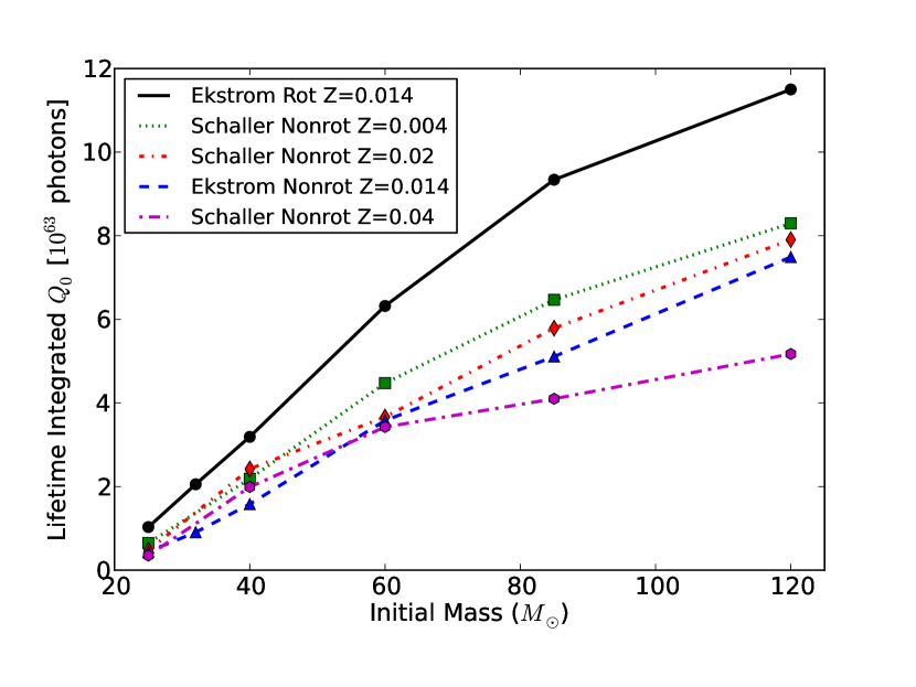
Figure 7.— Lifetime-integrated number of H-ionizing photons, $Q_{0}^{\rm(tot)}(m)$, for three older evolutionary tracks, labeled “Schaerer” and taken from Schaller et al. (1992) at three different metallicities. For comparison, we show LyC production for two new solar-metallicity tracks (Ekström et al. 2012) computed with and without rotation.

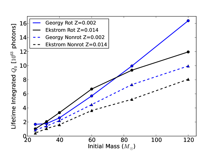
Figure 8.— Comparison of lifetime-integrated LyC photon production, $Q_{0}^{\rm(tot)}(m)$, for new evolutionary tracks (Ekström et al. 2012; Georgy et al. 2013), with and without rotation, at solar ($Z=0.014$) and sub-solar ($Z=0.002$) metallicity.

Figure 8 compares $Q_{0}^{\rm(tot)}(m)$ for the new rotating and non-rotating tracks (Ekström et al. 2012; Georgy et al. 2013) at the two available metallicities, $Z=0.014$ and $Z=0.002$. Here again, we see that LyC production is elevated by $\sim 50$% for models with rotation over most of the mass range of O-stars. Our integrations with the new non-rotating tracks produce $Q_{0}^{\rm(tot)}(m)$ curves (two dashed lines in Figure 8) that are nearly linear with mass, while production rates with the older tracks (Schaller et al. 1992) flatten out for the $85\;M_{\odot}$ and $120\;M_{\odot}$ models. Interestingly, the new rotating-track models of Georgy et al. (2013) show considerably more LyC photons at $120\;M_{\odot}$, continuing the linear trend of $Q_{0}^{\rm(tot)}(m)$. However, those tracks were computed at low metallicity ($Z=0.002$) which may explain part of the increase in LyC production.

In general, stars with lower metallicity have a reduced rate of CNO-cycle burning, which results in a contraction and heating of the star’s core and increased burning through the proton-proton chain. Consequently, the surface temperature is hotter and the star produces more ionizing photons. Additionally, fewer metals in the atmosphere produce less line blanketing, which alters the spectral shape in the UV and EUV. The effects of stellar rotation on LyC production and $Q_{0}^{\rm(tot)}(m)$ arise partly from the prolongation of hydrogen burning, as new fuel is mixed into the core. Rotating models are more luminous, because of their larger convective cores, and their surfaces are hotter owing to enhanced helium abundances. As our calculations bear out, the ionizing fluxes are greater, as are their lifetime integrated LyC productions. Thus, owing to the complicated evolutionary tracks of massive stars through different ranges of parameters ($T_{\rm eff}$, $\log g$, $L$, $R_{*}$) there are multiple factors contributing to the increase of LyC production found at low metallicity and with enhanced rotation.

4.2. Integration Over Initial Mass Functions

With these data and the IMF of a stellar population, we can calculate the number of LyC photons produced per solar mass of star formation. To do this, we integrate the IMF, $\xi(m)$, multiplied by the lifetime integrated photon number $Q_{i}(m)$ for the three ionization continua ($i=0,1,2$). We also consider three different IMFs. The first is adapted from Salpeter (1955), who found $\xi(m)=Km^{-\alpha}$, with index $\alpha=2.35$ for stars between 0.4 $M_{\odot}$ and 10 $M_{\odot}$. We extend the mass range to $0.1\leq m\leq 120$ ($m$ in $M_{\odot}$) and take $K$ as a normalization constant. The Salpeter function is the steepest of the three IMFs, maintaining the same index through its entire mass range, whereas recent surveys suggest a turnover at low mass. The second IMF is from Kroupa (2001), a piecewise-continuous power law, split into three mass ranges, each with a different value of $\alpha$. We integrate over the two stellar mass ranges between 0.08 $M_{\odot}$ and 120 $M_{\odot}$, in which $\alpha=1.3$ ($0.08\leq m\leq 0.5$) and $\alpha=2.3$ ($0.5\leq m\leq 120$). The third IMF is from Chabrier (2003), with the same index ($\alpha=2.3$) for stars with $m>0.5$. For $0.08<m\leq 0.5$ this IMF has the more complicated log-normal form: $\xi(m)=A\exp[-(\log m-\log m_{c})^{2}/2\sigma^{2}]$.

Table 2 summarizes the results of our calculations for various combinations of IMF, metallicities, and evolutionary tracks, with and without rotation. The LyC production efficiency is defined as the lifetime-integrated number of ionizing photons per solar mass of star formation. We list three versions of these parameters, $Q_{\rm LyC}$, $Q_{\rm HeI}$ and $Q_{\rm HeII}$, corresponding to the ionizing continua of H I, He I, and He II. These are sensitive to the sets of model atmospheres and stellar tracks, as well as the IMF index ($\alpha$) at the high-mass end, and the integrated mass range ($m_{\rm min}$ and $m_{\rm max}$).

4.3. Reionization and LyC Production Effiicency

We now apply the new stellar models to reionization by comparing our calculated values of $Q_{\rm LyC}$ to the LyC production efficiencies calculated by Shull et al. (2012). The ionizing photons $Q_{\rm LyC}$ produced per $M_{\odot}$ of star formation are important for determining when IGM reionization was mostly complete. This can be assessed by finding the critical star formation rate density (Madau et al. 1999) necessary to keep the IGM ionized, balancing photoionizations with hydrogen recombinations. The critical density was recently evaluated (Shull et al. 2012) using updated estimates for LyC production rates ($Q_{\rm LyC}$) and LyC escape fraction ($f_{\rm esc}$) as well as IGM structure (density and temperature). Hydrogen (case-B) recombination rates depend on electron temperature as $T^{-0.845}$ and are enhanced by a “clumping factor” $C_{H}\equiv\langle n^{2}\rangle/\langle n\rangle^{2}$. With calculations of IGM clumping, escape fraction, and LyC production efficiencies, Shull et al. (2012) suggested fiducial values of $C_{H}\approx 3$, $f_{\rm esc}\approx 0.2$, $T_{e}=(10^{4}~{}{\rm K})T_{4}$, and LyC efficicncies $Q_{\rm LyC}=0.004$ (in $10^{63}$ photons per $M_{\odot}$) to find

$$\dot{\rho}_{\rm SFR} = (0.018\;M_{\odot}\;\rm yr^{-1}\;\rm Mpc^{-3})\left[\frac{(1+z)}{8}\right]^{3}$$ (3)

$$\times \left(\frac{C_{\rm H}/3}{\textit{f}_{\rm esc}/0.2}\right)\left(\frac{0.004}{Q_{\rm LyC}}\right)T^{-0.845}_{4}\;.$$

The value of $f_{\rm esc}$ for low-mass galaxies with a cloudy ISM has been estimated to be 10-20% (Fernandez & Shull 2011). Depending on choices of $C_{H}$ and $T_{e}$, the escape fraction needs to be at least 10% in order to complete IGM reionization by $z=7$ (Shull et al. 2012; Robertson et al. 2013; Finkelstein et al. 2013).

In our study, we have explored three factors that affect the LyC production efficiency: (1) decreases in stellar metallicity; (2) increases in stellar rotation; (3) shape of the IMF. From our new calculations of ionizing photon production rates we assess how LyC production efficiency is affected by choices of stellar tracks (rotation, metallicity), model atmospheres, and IMF. By comparing results for various combinations of these parameters, we findthe general trends with metallicity and rotation. We currently have the full range of evolutionary tracks at two metallicities, solar and sub-solar. We integrate over three IMFs, labeled in Table 2 as $(1,2,3)$ corresponding to (Salpeter, Kroupa, Chabrier). The stellar tracks are labeled as $(4,5,6)$ corresponding to (Schaller 1992, Ekström 2012, Georgy 2013). The latter two tracks come with and without rotation. Our results (Figures 7 and 8) show that for each set of non-rotating evolutionary tracks their rotating counterparts produce more photons. Metallicity is less important for the overall efficiency, $Q_{\rm LyC}$, although it can be a factor at specific masses. For the 40 $M_{\odot}$ and 60 $M_{\odot}$ models with rotation, the solar metallicity models produce more photons than the sub-solar models. Owing to the power-law decrease of the IMF at high masses, this small difference in ionizing photon production results in the solar-metallicity models producing slightly more photons per solar mass. For fixed evolutionary tracks, metallicities, and model atmospheres, adopting the Kroupa or Chabrier IMF increases the LyC efficiency by factors of 1.56 and 1.64, respectively, relative to the Salpeter IMF.

We now perform a detailed comparison of our computed values of $Q_{\rm LyC}$ to the fiducial value $Q_{\rm LyC}=0.004$ suggested by Shull et al. (2012). With different combinations of IMFs and evolutionary tracks, $Q_{\rm LyC}$ extends from 0.00315 to 0.00940 for solar metallicity and from 0.00402 to 0.00910 for sub-solar metallicity (Table 2). This spread in efficiencies translates to a factor of 3 in critical SFR density. Values of $Q_{\rm LyC}$ computed with rotating evolutionary tracks and the Kroupa IMF were at the upper end of the range. One can further analyze these $Q$-values to separate the effects of reduced metallicity from those of rotation. The three IMFs only change the overall normalization, because of their different mass-loading by low-mass stars. Because the Salpeter IMF includes more low-mass stars, the absolute values of $Q_{\rm LyC}$ are reduced; these stars add mass but produce few ionizing photons.

First, we examine the effects of metallicity. For the “old” non-rotating tracks (Schaller et al. 1992) at solar metallicity ($Z=0.020$) we find $Q_{\rm LyC}=0.00367$, 0.00572, and 0.00370 for the three IMFs (1,2,3) considered here (Salpeter, Kroupa, and Chabrier, respectively). For the new non-rotating tracks (Ekström et al. 2012) at sub-solar metallicity ($Z=0.004$) we find $Q_{\rm LyC}=0.00399$, 0.00623, and 0.00402 for IMFs (1,2,3). Taking the appropriate ratios for the old tracks and corresponding model atmospheres, we find that decreasing the metallicity from solar ($Z=0.02$) to sub-solar ($Z=0.004$) increases the LyC efficiencies by only 9%. That is, the ratio $Q_{\rm LyC}({\rm subsolar})/Q_{\rm LyC}({\rm solar})=1.09$ for all three IMFs. However, performing the same calculation for the new non-rotating tracks (Ekström et al. 2012; Georgy et al. 2013), we find a 34% increase at sub-solar metallicity, with $Q_{\rm LyC}({\rm subsolar})/Q_{\rm LyC}({\rm solar})=1.34$. For the new rotating tracks, the LyC efficiencies at solar and sub-solar metallicity are essentially the same, with $Q_{\rm LyC}({\rm subsolar})/Q_{\rm LyC}({\rm solar})=0.97$ for all three IMFs. Chabrier and Kroupa IMFs have the same power-law slope for high mass ($\alpha=2.3$), but each uses a different fit for low-mass stars. The Chabrier IMF has more low-mass stars compared to the Kroupa IMF and therefore more stellar mass that is not producing ionizing photons. Next, we examine the effect of rotation on $Q_{\rm LyC}$ at fixed metallicity. For all three IMFs, the evolutionary tracks with rotation produce more ionizing photons per solar mass. At solar metallicity ($Z=0.014$) the Ekström et al. (2012) tracks and corresponding model atmospheres yield 87% higher LyC efficiency, with $Q_{\rm LyC}({\rm rot})/Q_{\rm LyC}({\rm nonrot})=1.87$. At sub-solar metallicity ($Z=0.002$) the Georgy et al. (2013) tracks and corresponding atmospheres were 35% more efficient in LyC production, with $Q_{\rm LyC}({\rm rot})/Q_{\rm LyC}({\rm nonrot})=1.35$.

As a general conclusion, we find that increased stellar rotation is more important than reduced metallicity in boosting the LyC efficiency. By comparing subsets of tracks, metallicities, and IMFs, we can recover more specific results. We label the LyC production efficiencies by $Q_{\rm LyC}{\rm(IMF,Tracks)}$, where IMFs and tracks are defined as in Table 2 (1 = Salpeter, 2 = Kroupa, 3 = Chabrier) with non-rotating tracks labeled by (4 = Schaller; 5 = Ekström) and rotating tracks by (5 = Ekström, 6 = Georgy). For the relevant combinations of parameters, we find the following efficiencies for “non-rotating, solar metallicity” stellar populations:

$$Q_{\rm LyC}(1,4)=0.00367\;\;Q_{\rm LyC}(2,4)=0.00572$$

$$Q_{\rm LyC}(3,4)=0.00370\;\;(Z=0.020)$$

$$Q_{\rm LyC}(1,5)=0.00322\;\;Q_{\rm LyC}(2,5)=0.00503$$

$$Q_{\rm LyC}(3,5)=0.00325\;\;(Z=0.014)$$ (4)

The range of $Q_{\rm LyC}$ between $0.00322-0.00572$ arises primarily from the choice of IMF, which affects the “mass-loading” at the low end. Next, we make a similar tabulation for “non-rotating, sub-solar metallicity” populations (either $Z=0.004$ or $0.002$):

$$Q_{\rm LyC}(1,4)=0.00399\;\;Q_{\rm LyC}(2,4)=0.00623$$

$$Q_{\rm LyC}(3,4)=0.00402\;\;(Z=0.004)$$

$$Q_{\rm LyC}(1,6)=0.00433\;\;Q_{\rm LyC}(2,6)=0.00676$$

$$Q_{\rm LyC}(3,6)=0.00436\;\;(Z=0.002)$$ (5)

As before, the range of $Q_{\rm LyC}$ from $0.00399-0.00676$ arises from the assumed IMF. Finally, for the rotating tracks at both solar and sub-solar metallicities, we find:

$$Q_{\rm LyC}(1,5)=0.00603\;\;Q_{\rm LyC}(2,5)=0.00940$$

$$Q_{\rm LyC}(3,5)=0.00607\;\;(Z=0.014)$$

$$Q_{\rm LyC}(1,6)=0.00583\;\;Q_{\rm LyC}(2,6)=0.00910$$

$$Q_{\rm LyC}(3,6)=0.00588\;\;(Z=0.002)$$ (6)

The range of $Q_{\rm LyC}$ from $0.00583-0.00940$ arises mainly from the assumed IMF.

Adopting an IMF with fewer low-mass stars or using tracks with increased stellar rotation produces larger boosts in LyC efficiency than sub-solar metallicity. For non-rotating stars at solar metallicity, a typical value is $Q_{\rm LyC}=0.004\pm 0.002$, as found in our previous study (Shull et al. 2012). Including stellar rotation could increase the efficiency to $Q_{\rm LyC}=0.0075\pm 0.0015$, although those stellar tracks assumed a single value of rotation at 40% of breakup, which may be excessively high. Allowing for the range in $Q_{\rm LyC}$ efficiencies produced by assumptions about IMF, metallicity, and rotation, we recommend adopting an overall LyC production efficiency of $Q_{\rm LyC}=0.006\pm 0.002$ in Equation (3), or a photon production calibration of $(6\pm 2)\times 10^{60}$ LyC photons per $M_{\odot}$ of star formation. This is equivalent to a SFR calibration of $10^{53.3\pm 0.2}$ photons s^-1 for SFR in $M_{\odot}$ yr^-1 and represents a 50% increase over previous estimates. With the new LyC rates, the critical SFR to maintain reionization can be rewritten

$$\dot{\rho}_{\rm SFR} = (0.012\;M_{\odot}\;\rm yr^{-1}\;\rm Mpc^{-3})\left[\frac{(1+z)}{8}\right]^{3}$$ (7)

$$\times \left(\frac{C_{\rm H}/3}{\textit{f}_{\rm esc}/0.2}\right)\left(\frac{0.006}{Q_{\rm LyC}}\right)T^{-0.845}_{4}\;.$$

The 50% boost in LyC production efficiency is an important ingredient in assessing whether IGM reionization was complete by $z\approx 7$, as suggested by recent observations (Oesch et al. 2014; McLure et al. 2013; Robertson et al. 2013; Finkelstein et al.  2012).

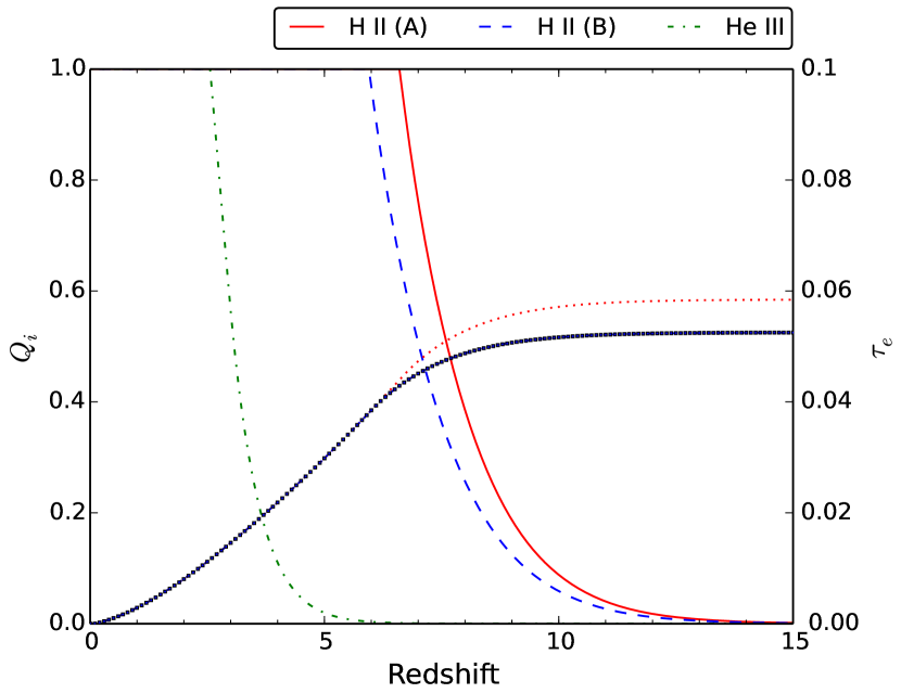
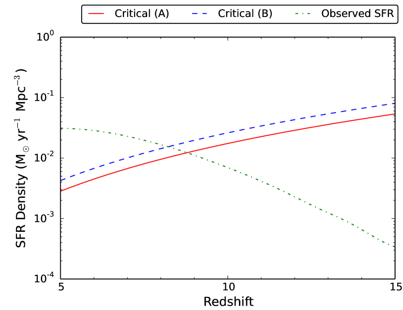
Figure 9.— Reionization histories and critical SFRs for two LyC production efficiencies, computed with our reionization simulator (Shull et al. 2012). Left: Ionized volume fraction $Q_{i}$ and integrated CMB optical depth, $\tau_{e}$, to electron scattering for two LyC production rates: $Q_{\rm LyC}=0.006$ (solid red curve, model A) and $Q_{\rm LyC}=0.004$ (dashed blue curve, model B), both in $10^{63}$ photons per $M_{\odot}$ of star formation. The dot-dashed curve at $z<5$ follows the He II history, governed by quasars and completed at $z\approx 3$. Right: Critical SFR densities required to maintain IGM ionization compared to observed and extrapolated SFR (green dot-dashed curve). Reionization models (assume clumping factor $C_{H}=3$, LyC escape fraction $f_{\rm esc}=0.2$, and electron temperature $T_{e}=20,000$ K. The SFR history comes from the galaxy luminosity function (Trenti et al. 2010) extrapolated down to absolute magnitude $M_{\rm AB}=-10$ in rest-frame UV and converted to SFR density using the prescription in Madau et al. (1999).

These considerations are illustrated in Figure 9, which shows the reionization histories and critical SFR densities derived with the reionization simulator developed in a previous study (Shull et al. 2012). The left panel shows the redshift evolution of the ionized volume fraction, $Q_{i}(z)$, for two values of LyC production efficiency, $Q_{\rm LyC}=0.004$ (the old standard) and $Q_{\rm LyC}=0.006$ (the new efficiency). Accompanying curves show the evolution of CMB optical depth, $\tau_{e}$, to electron scattering, an integral constraint on the ionization history. These two models, labeled A and B, adopt identical physical parameters, $C_{H}=3$, $f_{\rm esc}=0.2$, and $T_{e}=20,000$ K. The SFR history follows that of Trenti et al. (2010) with the galaxy luminosity function extrapolated down to absolute magnitude $M_{\rm AB}=-10$ in the rest-frame UV. The curve at $z<5$ follows the He II history, which is governed by quasars, with He II reionization completed at $z\approx 3$. The right panel compares $\dot{\rho}_{\rm SFR}$, the critical SFR density from Equation (7), to the observed (and extrapolated) SFR density. The increased LyC production efficiency shifts the evolution in ionized volume fraction, $Q_{i}(z)$, toward higher redshifts. One can therefore offset $Q_{\rm LyC}\approx 0.006$ against the combination of physical parameters, $(C_{H}/f_{\rm esc})T_{4}^{-0.845}\approx 8.35$ in this case. With the elevated LyC efficiency (model A), full reionization ($Q_{i}\approx 1$) occurs at $z\approx 7$, and the “observed and extrapolated SFR exceeds $\dot{\rho}_{\rm SFR}$ at $z<9$. The ionization history can be altered with various combinations of physical parameters and by different extrapolations to low-luminosity galaxies.

4.4. He I and He II Continuum Photon Luminosities

From the same data used to determine LyC photon fluxes, we only need to change integration limits to compute fluxes in the He I and He II continua. The calculation of $Q_{1}(m)$, the He I-ionizing photon production for each initial mass, follows the same procedure as for $Q_{0}(m)$ using Equation (1) with $\lambda_{\rm lim}=504.259$ Å. The $Q_{1}(m)$ curves with solar metallicity (Figure 10) have a similar shape to the H I Lyman continuum curves in Figures 7 and 8. In both cases, the photon production increases with mass but flattens out at $120\;M_{\odot}$. Because the photons are in the Wien limit ($h\nu\gg kT_{\rm eff}$) of the Planck function, the intensity of radiation decreases exponentially in this short-wavelength range. Consequently the photon production rates for He I ionization are significantly less than the H I continuum rates, by up to an order of magnitude. The comparison between the new evolutionary tracks at two different metallicities follows a different trend. The first difference is the behavior of the two most massive models in the sub-solar rotating model. Instead of flattening with increasing mass, the models seem to produce a rapidly increasing number of ionizing photons. The other sets of evolutionary tracks produce rather linear $Q_{1}(m)$ curves.

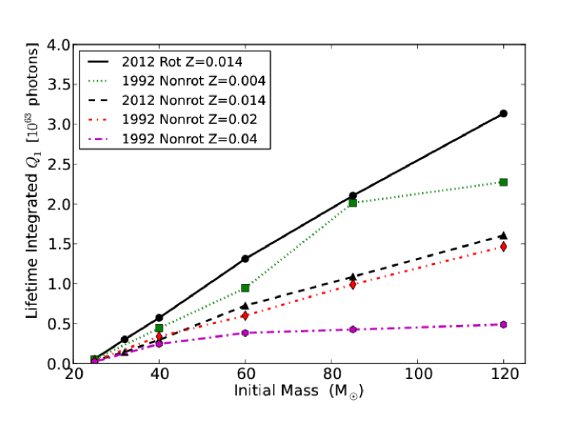
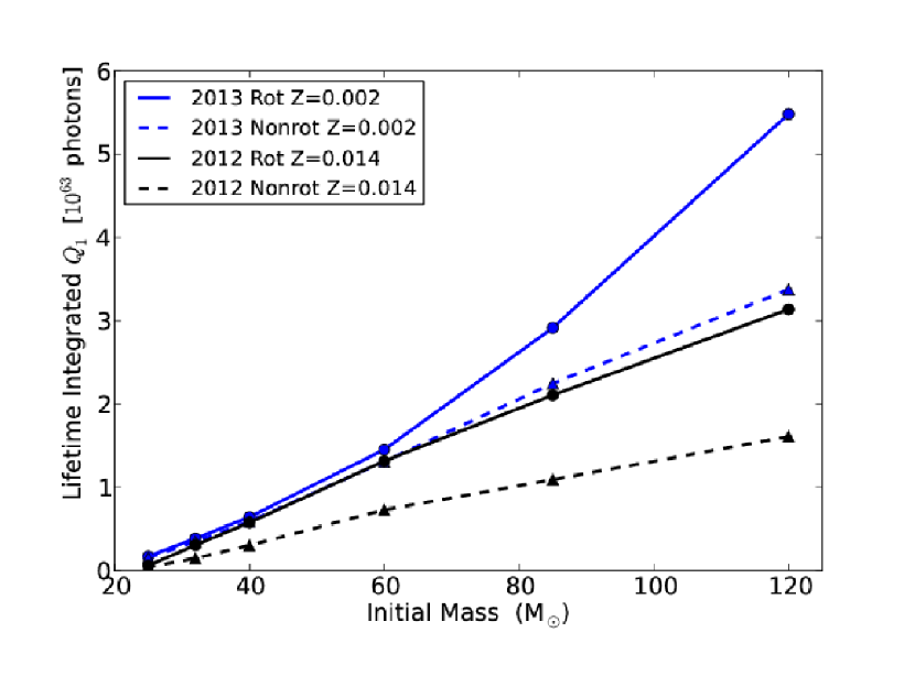
Figure 10.— Lifetime-integrated He I continuum photon production $Q_{1}^{\rm(tot)}(m)$ in $10^{63}$ photons vs. initial mass for several evolutionary tracks. Top: former standard tracks compared to new rotating and non-rotating solar metallicity tracks. “1992 Nonrot” tracks from Schaller et al. (1992), and “2012 Rot/Nonrot” tracks from Ekström et al. (2012). Bottom: new rotating and non-rotating tracks at solar and sub-solar metallicity. “2013 Rot/Nonrot” tracks are from Georgy et al. (2013).

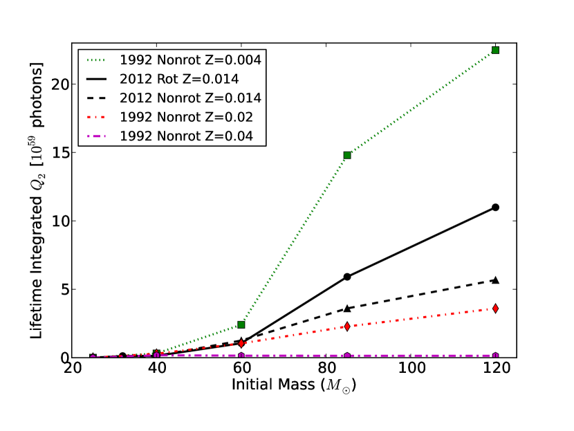
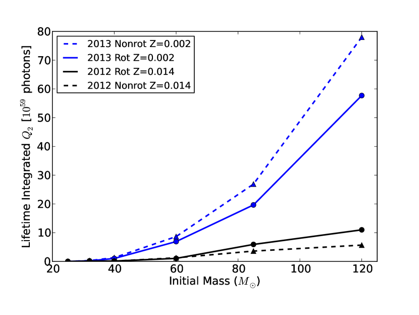
Figure 11.— Lifetime-integrated He II continuum photon production $Q_{2}^{\rm(tot)}(m)$ vs. initial mass. Top panel: Comparison of old evolutionary tracks (Schaller et al. 1992) and new solar metallicity rotating and non-rotating evolutionary tracks (Ekström et al. 2012). Bottom: Comparison of new rotating and non-rotating evolutionary tracks at solar and sub-solar metallicity (Ekström et al. 2012; Georgy et al. 2013).

From the data in Table 2, we find a factor of three range in $Q_{\rm HeI}$ depending on choice of IMF, metallicity, and rotation. For the “old” non-rotating models (Schaller et al. 1992 tracks) we find $Q_{\rm HeI}\approx(0.5-0.9)\times 10^{60}$ photons per $M_{\odot}$ at solar metallicity. At sub-solar metallicities, the He I continuum production is higher by 60% with $Q_{\rm HeI}({\rm subsolar})/Q_{\rm HeI}({\rm solar})=1.6$. In the newer non-rotating tracks (Ekström et al. 2012 and Georgy et al. 2013) $Q_{\rm HeI}$ is a factor of 2 larger. For the new rotating models, the range is $Q_{\rm HeI}\approx(1.1-1.7)\times 10^{60}$ photons per $M_{\odot}$ at solar metallicity and 32% higher at sub-solar metallcity. Rotation elevates $Q_{\rm HeI}$ at fixed metallicity for all three IMFs. At solar metallicity ($Z=0.014$) the Ekström et al. (2012) tracks and corresponding atmospheres yield 94% higher efficiency, with $Q_{\rm HeI}({\rm rot})/Q_{\rm HeI}({\rm nonrot})=1.94$. At sub-solar metallicity ($Z=0.002$) the Georgy et al. (2013) tracks and corresponding atmospheres were 22% more efficient, with $Q_{\rm HeI}({\rm rot})/Q_{\rm HeI}({\rm nonrot})=1.22$. The overall He I efficiency ranges are comparable to those for $Q_{\rm LyC}$. The recommended median value is $Q_{\rm HeI}=0.6\times 10^{60}$ photons per $M_{\odot}$ (non-rotating, solar metallicity) with significant enhancements (60-110%) at lower metallicity, unlike for the total LyC. The enhancements in $Q_{\rm HeI}$ due to rotation are comparable to those for the LyC, at both solar metallicity (90% boosts) and sub-solar (22-35% boosts).

Finally, we compute the He II-ionizing photon fluxes $Q_{2}(m)$ using Equation (1) with $\lambda_{\rm lim}=227.838$ Å. At higher ionization energies, the production of He II-continuum photons is several orders of magnitude lower than for H I or He I continua. Curves of $Q_{2}(m)$ vs. initial mass are shown in Figure 11 for rotating and non-rotating evolutionary tracks at solar and sub-solar metallicity. Several features distinguish $Q_{2}(m)$ from $Q_{0}(m)$ or $Q_{1}(m)$ curves. First, the lower metallicity models produce significantly more photons than models with higher metallicity. This is consistent with our expectations and the results of the $Q_{0}(m)$ and $Q_{1}(m)$ calculations. The next distinction is that at sub-solar metallicity, the non-rotating models produce more He II continuum photons than corresponding rotating models. This is different from our expectations and the trends from solar-metallicity models. We can understand this discrepancy by examining the behavior of the sub-solar metallicity tracks, in which non-rotating models have a higher effective temperature and luminosity for roughly 1.5 Myr, which constitutes a majority of their lifetimes. At the high energies of the He II continuum, the spectrum is quite sensitive to $T_{\rm eff}$.

The recommended value for He II is $Q_{\rm HeII}=1\times 10^{56}$ photons per $M_{\odot}$ (non-rotating, solar metallicity). The enhancements in $Q_{\rm HeII}$ due to rotation are a factor of 1.48 at solar metallicity, but reduced by a factor of 0.76 at sub-solar metallicity. Using the same pairwise comparisons as used above for $Q_{\rm LyC}$ and $Q_{\rm HeI}$, we find large boosts in $Q_{\rm HeII}$ at lower metallicity. The ratio $Q_{\rm HeII}({\rm subsolar})/Q_{\rm HeII}({\rm solar})=4.65$ for old non-rotating tracks (and corresponding atmosphere models) as well as for the new rotating tracks.

4.5. LyC Spectra in Model OB Associations

The spectral evolution of an ensemble of stars of various masses can be combined through an IMF and followed over time. Such spectral synthesis codes are valuable tools for ultraviolet spectral libraries (Robert et al. 1993; Rix et al. 2004; Leitherer et al. 2014) and stellar population synthesis codes such as Starburst99 (Leitherer et al. 1999). Figure 12 shows a series of spectra for a cluster starburst containing $10^{5}~{}M_{\odot}$ in which the stars follow a Salpeter IMF ($0.1\leq m\leq 120$). The two panels show model spectra at times $t=$ 0, 1, 3, 5, and 7 Myr after a coeval burst of star formation, using evolutionary tracks with rotation, at solar metallicity ($Z=0.014$ from Ekström et al. 2012) and at sub-solar metallicity ($Z=0.014$ from Georgy et al. 2013). These models were created by Monte-Carlo sampling of stars for each mass for which we have an evolutionary track ($m=20$, 25, 32, 40, 60, 85, 120). For the Salpeter differential mass distribution, $\xi(m)=Km^{-\alpha}$ with $\alpha=2.35$, the fraction of stars above mass $m$ is given by

$$\frac{N(>m)}{N}=\frac{[m^{-(\alpha-1)}-m_{\rm max}^{-(\alpha-1)}]}{[m_{\rm min}^{-(\alpha-1)}-m_{\rm max}^{-(\alpha-1)}]}\;\;.$$ (8)

The constant $K$ is normalized to the total cluster mass $M=5.862K$, and the total number of stars $N=16.582K$ for mass limits $m_{\rm min}=0.1$ and $m_{\rm max}=120$. For $M=10^{5}~{}M_{\odot}$, we expect a mean number $\bar{N}=282,500$ stars and mean stellar mass $\langle m\rangle=M/N=0.354$ $M_{\odot}$. In many of our Monte-Carlo samples, the numbers fluctuate about this value, with small numbers at the high-mass end of the IMF. The mean numbers of stars at the high-mass end are: $N(>60~{}M_{\odot})\approx 30$ and $N(>100~{}M_{\odot})\approx 5$. If the upper mass was extended to $m_{\rm max}=200$, we would expect 40 stars above 60 $M_{\odot}$ and 15 stars above 100 $M_{\odot}$. As discussed earlier, the existence of these very massive stars is controversial, owing to resolution effects. Moreover, the LyC from stars at $m>100$ $M_{\odot}$ may not escape the embedded cloud from which they formed, or from the dense gas produced in mass-loss episodes or binary mergers (Smith 2014). We therefore do not consider stars above the 120 $M_{\odot}$ track.

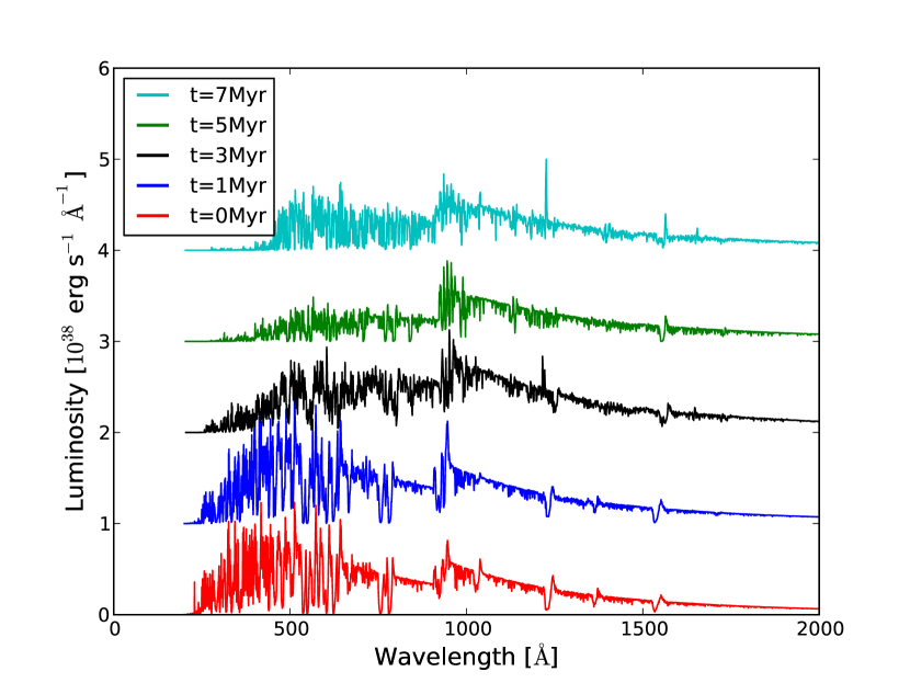
Figure 12.— Overlaid spectral distributions in specific luminosity, $L_{\lambda}$ in $10^{38}$ erg s^-1 Å^-1, for Monte-Carlo models of a star-forming cluster. We assume $10^{5}~{}M_{\odot}$ of stars with Salpeter IMF ($0.1\leq m\leq 120$) and use evolutionary tracks with rotation and model atmospheres at the appropriate metallicities. Top: Solar metallicity ($Z=0.014$, Ekström et al. 2012). Bottom: Sub-solar metallicity ($Z=0.002$, Georgy et al. 2013). Each curve is offset by 1.0 (in $10^{38}$ units) plotted, from bottom to top, at times $t=$ 0, 1, 3, 5, and 7 Myr after a coeval burst of star formation. See Section 4.5 for details.

Figure 13.— Monte-Carlo simulations, as in Fig. 12, of the time evolution of LyC production rate $Q_{0}(t)$ [photons s^-1] in a cluster with $10^{5}~{}M_{\odot}$, formed coevally in a Salpeter mass distribution ($0.1<m<120$). We use evolutionary tracks at solar metallicity with rotation ($Z=0.014$, Ekström et al. 2012) and show two runs with different selections of stellar masses, from initial random-number seeds. Late-time spikes ($3.5-6.2$ Myr) arise from the post-main-sequence evolution of stars with 40-60 $M_{\odot}$.

The spectra of each model are calculated from the star’s basic parameters on the evolutionary tracks, multiplied by the number of stars for each mass and added to the total spectra. The stars are randomly chosen, weighted by the IMF, until the total mass of the cluster is $10^{5}$ $M_{\odot}$. Owing to the rarity of O-stars at the upper end of the IMF, some models had no stars above 100 $M_{\odot}$. The LyC fluxes do not fade until after 5–7 Myr (Figure 13) owing to their post main-sequence evolution to O supergiants. However, fluxes at the shortest wavelengths ($\lambda<504$ Å) decrease after $\sim 5$ Myr.

As noted in Section 3.2, extragalactic observers have calibrated escaping LyC radiation from the flux-density ratios, $F(912^{-})/F(912^{+})$ at the Lyman edge, and $F(1500)/F(910)$, the far-UV-to-LyC ratio at 1500 Å  and 900 Å. These computed flux ratios are listed in Table 3 for model clusters calculated with rotating-star models at solar metallicity ($Z=0.014$) and sub-solar metallicity ($Z=0.002$). For coeval starburst models, the intrinsic flux decrement at the 912 Å Lyman edge ranges from $F(912^{-})/F(912^{+})\approx 0.4-0.7$ over the first 5 Myr for both solar and sub-solar metallicities. The far-UV (1500 Å) to LyC (900 Å) ratio ranges from $F(1500)/F(900)\approx 0.4-0.7$ over the same time period. In their studies of escaping LyC from starburst galaxies at $z\approx 3$, Steidel et al. (2001) defined a relative fraction of escaping LyC photons normalized to escaping 1500 Å photons:

$$f_{\rm esc,rel}=\frac{[F(1500)/F(900)]_{\rm int}}{[F(1500)/F(900)]_{\rm obs}}\;\exp(\tau_{\rm IGM,900})\;,$$ (9)

where $[F(1500)/F(900)]_{\rm int}$ is the intrinsic ratio of non-ionizing, far-UV (1500 Å) photons to ionizing photons (at 900 Å) and $\tau_{\rm IGM,900}$ is the line-of-sight optical depth of the intergalactic medium to LyC photons at 900 Å. The intrinsic spectral shape for massive stars above and below the Lyman edge is not well constrained by observations, and one must rely on stellar atmosphere models and population synthesis. Both Steidel et al. (2001) and Inoue et al. (2005) adopted an intrinsic ratio $F(1500)/F(910)=3.0$. Because our (1500 Å/900 Å) ratios are considerably lower (0.4-0.5) this will reduce the inferred escape fractions in high-redshift starburst galaxies, which are proportional to the assumed intrinsic ratio. This decrease in the intrinsic ratio may resolve the paradoxical inference (Shapley et al. 2006), who found a corrected flux ratio, $F(1500)/F(900)\approx 2.9$ implying that $f_{\rm esc}$ is greater than 100%. After 5–7 Myr, when the most massive O-type stars evolve off the main sequence and eventually die, the (1500-to-900 Å) flux ratios begin to increase.

5. DISCUSSION AND CONCLUSIONS

This work provides an update of the production rates of ionizing photons from massive stars, based on a new generation of stellar evolutionary tracks coupled to modern stellar atmosphere models. For a range of parameters (tracks, metallicities, rotation), we find a 50% increase in the LyC production efficiencies compared to previous calibrations. The new stellar tracks from the Geneva group were calculated for both solar and sub-solar metallicities, and they also examined the effects of stellar rotation with surface velocities 40% of breakup. For the grid points ($T_{\rm eff},\log g$) on these tracks, we computed model atmospheres with the non-LTE code WM-basic, which treats 3D expanding atmospheres and line-blanketing by lines of heavy elements whose metallicities were consistent with those in the stellar tracks. We computed the production rates of ionizing photons in the ionizing continuum of hydrogen, as well as of He I and He II, and their dependence on metallicity, rotation, and initial stellar mass. Next, we integrated these rates over three different IMFs (Salpeter, Kroupa, Chabrier) to derive LyC photon production efficiencies, $Q_{\rm LyC}$, in units of LyC photons per solar mass of star formation.

Our calculations used the recent grids of evolutionary tracks from the Geneva group, who made specific assumptions about stellar mass loss rates and rotation. These grids could be revised in the future, to account for improved parameterization of mass-loss rates, binary evolution, and the upper extent of the IMF. Recent observations of massive stars have introduced uncertainties in mass-loss rates, particularly in late (WR) stages (Gräfener & Vink 2013; Smith 2014). Binaries could affect the stellar populations owing to tides, mass transfer, and mergers (de Mink et al. 2013). Some effects of stellar mergers are effectively included in tracks with increased rotation. After considering a range of metallicities and the effects of stellar rotation, the main conclusions of our study can be summarized as follows:

1. By coupling new stellar evolutionary tracks at several metallicities, with and without rotation, to non-LTE model atmospheres, we find a range of LyC photon production efficiencies $Q_{\rm LyC}=[3.1-9.4]\times 10^{60}$ photons per $M_{\odot}$ of star formation. The median LyC production efficiency is $(6\pm 2)\times 10^{60}$ LyC photons per $M_{\odot}$, an average increase of 50% from previous models.

2. The new LyC efficiency is equivalent to a SFR calibration of $10^{53.3\pm 0.2}$ photons s^-1 per $M_{\odot}$ yr^-1. With these new rates, the critical SFR density in a clumpy medium can be written $\dot{\rho}_{\rm SFR}=(0.012\;M_{\odot}\;{\rm yr}^{-1}\;{\rm Mpc}^{-3})[(1+z)/8]^{3}(C_{\rm H}/3)(0.2/f_{\rm esc})(0.006/Q_{\rm LyC})T^{-0.845}_{4}$, scaled to fiducial values of IGM clumping factor $C_{H}=3$, LyC escape fraction $f_{\rm esc}=0.2$, and electron temperature $T_{e}=10^{4}$ K.

3. The higher LyC efficiencies make it easier to complete reionization by $z\approx 7$ for various physical parameters $C_{H}$, $f_{\rm esc}$, $T_{e}$ and extrapolations of the galaxy luminosity function to magnitudes well below those observed in the HST/WFC3 deep fields. For LyC efficiency $Q_{\rm LyC}=6\times 10^{60}$ photons per $M_{\odot}$, reionization is complete by $z=7$ for $(C_{H}/f_{\rm esc})\approx 15-30$ and $T_{e}=(1-2)\times 10^{4}$ K.

4. We also computed efficiencies for He I and He II continua. For He I, we find $Q_{\rm HeI}=0.6\times 10^{60}$ photons per $M_{\odot}$ (non-rotating, solar metallicity) with substantial (60-110%) enhancements at sub-solar metallicity and with rotation (90% boosts at solar metallicity and 22-35% boosts at sub-solar). For He II, we find $Q_{\rm HeII}=1\times 10^{56}$ photons per $M_{\odot}$ (non-rotating, solar metallicity) and a factor of 4.65 higher at low metallicity.

5. Because of the H I opacity in the upper stellar atmosphere, non-LTE models of stars with $T_{\rm eff}<50,000$ K exhibit 40-60% intrinsic LyC edges at 912 Å. These should be visible with next-generation UV missions that can observe escaping radiation in the rest-frame LyC of low-$z$ starburst galaxies.

6. Monte-Carlo simulations of starbursts find ratios of far-UV (1500 Å) to LyC (900 Å) flux density $F(1500)/F(900)\approx 0.4-0.5$ over the first 5 Myr, for models with metallicity $Z=0.014$ and $0.002$. The flux ratio at the Lyman edge $F(912^{-})/F(912^{+})\approx 0.4-0.7$ over the same time interval.

Several improvements could be made in future calculations. Additional stellar tracks at initial masses between 25 and 60 $M_{\odot}$, with rotation and super-solar metallicity would strengthen our results for the metallicity dependence of $Q_{\rm LyC}$. They would also provide a further basis of comparison to older super-solar evolutionary tracks (Schaller et al. 1992). Models with a range of rotation rates would be helpful, since rotation speeds at 40% of breakup may be excessive and produce ionizing SEDs inconsistent with nebular emission lines (Levesque et al. 2012). Our calculations rely on rotating tracks in which all stars have the same initial rotation. None of the current tracks include a description of magnetic fields, although that has not yet been shown to have a significant effect. Future stellar population models will treat rotation more realistically, with better understanding of their ionizing photon budgets.

Several changes in our computational scheme could also result in more accurate photon fluxes and production rates. When creating the grid ($\log g$, $T_{\rm eff}$) of model atmospheres, we continued adding models until we reached convergence in photon production rates. Adding more model atmospheres, up to one per time step of the evolutionary tracks, would create more precision. Another small effect is the contribution of ionizing photon production of lower mass stars. We currently consider models with masses $m$ $\geq 25$ $M_{\odot}$. Lower mass stars produce an order of magnitude or more fewer LyC photons. Filling in the grid at other metallicities and for additional masses between 35 $M_{\odot}$and 120 $M_{\odot}$ would be helpful. For reionization, the most important factors that could increase the total LyC production are the stellar populations at low metallicity, the extent of the upper main sequence, the influence of rapid rotation, and the role of binaries.

Table 1Ionizing Photon Production vs.  Initial Stellar Mass

Model Tracks	$(Z/Z_{\odot})$	$Q_{0}(120~{}M_{\odot})$	$Q_{0}(85~{}M_{\odot})$	$Q_{0}(60~{}M_{\odot}$)	$Q_{0}(40~{}M_{\odot})$	$Q_{0}(32~{}M_{\odot})$	$Q_{0}(25~{}M_{\odot})$
		($10^{63}$ phot)	($10^{63}$ phot)	($10^{63}$ phot)	($10^{63}$ phot)	($10^{63}$ phot)	($10^{63}$ phot)
Ekström (Rot)	0.014	11.5	9.34	6.32	3.19	2.06	1.03
Ekström (Non-Rot)	0.014	7.49	5.11	3.58	1.58	0.902	0.445
Georgy (Rot)	0.004	16.4	9.95	5.70	2.59	1.76	1.67
Georgy (Non-Rot)	0.004	9.95	7.31	4.47	2.19	1.43	0.871
Schaller (Non-Rot)	0.020	7.91	5.78	3.66	2.42	…	0.474
Schaller (Non-Rot)	0.004	8.29	6.46	4.47	2.18	…	0.648

Table 2Ionizing Photons with Various IMFs, Tracks, and Metallicities ($Z$)

Model	IMF	Tracks	Rot-Type	$m_{\rm min}$	$m_{\rm max}$	Slope	Metals	$Q_{\rm LyC}$	$Q_{\rm HeI}$	$Q_{\rm HeII}$
				($M_{\odot}$)	($M_{\odot}$)	$\alpha$	$Z$	($10^{61}$)	($10^{60}$)	($10^{56}$)
Solar	1	4	Nonrot	$0.1$	$120$	$2.35$	$0.020$	$0.367$	0.552	0.918
Solar	1	5	Rot	$0.1$	$120$	$2.35$	$0.014$	$0.603$	1.11	1.73
Solar	1	5	Nonrot	$0.1$	$120$	$2.35$	$0.014$	$0.322$	0.571	1.17
Solar	2	4	Nonrot	$0.01$	$120$	$2.3$	$0.020$	$0.572$	0.864	1.45
Solar	2	5	Rot	$0.01$	$120$	$2.3$	$0.014$	$0.940$	1.74	2.76
Solar	2	5	Nonrot	$0.01$	$120$	$2.3$	$0.014$	$0.503$	0.895	1.86
Solar	3	4	Nonrot	$0.01$	$120$	$2.3$	$0.020$	$0.370$	0.558	0.935
Solar	3	5	Rot	$0.01$	$120$	$2.3$	$0.014$	$0.607$	1.13	1.78
Solar	3	5	Nonrot	$0.01$	$120$	$2.3$	$0.014$	$0.325$	0.578	1.21
Sub-solar	1	4	Nonrot	$0.1$	$120$	$2.35$	$0.004$	$0.399$	0.884	4.25
Sub-solar	1	6	Rot	$0.1$	$120$	$2.35$	$0.002$	$0.583$	1.47	8.08
Sub-solar	1	6	Nonrot	$0.1$	$120$	$2.35$	$0.002$	$0.433$	1.21	10.7
Sub-solar	2	4	Nonrot	$0.01$	$120$	$2.3$	$0.004$	$0.623$	1.38	6.75
Sub-solar	2	6	Rot	$0.01$	$120$	$2.3$	$0.002$	$0.910$	2.31	12.8
Sub-solar	2	6	Nonrot	$0.01$	$120$	$2.3$	$0.002$	$0.676$	1.90	16.9
Sub-solar	3	4	Nonrot	$0.01$	$120$	$2.3$	$0.004$	$0.402$	0.896	4.36
Sub-solar	3	6	Rot	$0.01$	$120$	$2.3$	$0.002$	$0.588$	1.49	8.28
Sub-solar	3	6	Nonrot	$0.01$	$120$	$2.3$	$0.002$	$0.436$	1.22	10.9

Table 3Flux Ratios in Composite Cluster Spectra

Time	$F(912^{-})/F(912^{+})$	$F(912^{-})/F(912^{+})$	$F(1500)/F(900)$	$F(1500)/F(900)$
	$Z=0.014$	$Z=0.002$	$Z=0.014$	$Z=0.002$
0 Myr	0.54	0.58	0.472	0.455
1 Myr	0.57	0.71	0.457	0.438
3 Myr	0.65	0.71	0.506	0.404
5 Myr	0.39	0.41	0.777	0.727
7 Myr	0.50	0.31	0.630	1.03

References

- (1)
- (2) Asplund, M., Grevesse, N., Sauval, A. J., & Scott, P. 2009, ARA&A, 47, 481
- (3)
- (4) Bouwens, R. J., Illingworth, G, P., Oesch, P. A., et al. 2011, ApJ, 737, 90
- (5)
- (6) Bradley, L., Trenti, M., Oesch, P. A. et al. 2012, ApJ, 760, 108
- (7)
- (8) Caffau, E., Ludwig, H.-G., Steffen, M., et al. 2011, Solar Phys., 268, 255.
- (9)
- (10) Castor, J. J., Abbott, D. C., & Klein, R. I. 1975, ApJ, 195, 157
- (11)
- (12) Chabrier, G. 2003, PASP, 115, 763
- (13)
- (14) Charbonnel, C., Meynet, G., Maeder, A., et al. 1993, A&A, 101, 415
- (15)
- (16) Crowther, P. A. 2007, ARA&A, 45, 177
- (17)
- (18) Crowther, P. A., Schnurr, O., Hirschi, R., et al. 2010, MNRAS, 408, 731
- (19)
- (20) de Mink, S. E., Langer, N., Izzard, R. G., Sana, H., & de Koter, A. 2013, ApJ, 764, 166
- (21)
- (22) de Mink, S. E., Sana, H., Langer, N., Izzard, R. G., & Schneider, F. R.N. 2014, ApJ, 782, 7
- (23)
- (24) Ekström, S., Georgy, C., Eggenberger, P. et al. 2012, A&A, 537, A146
- (25)
- (26) Eldridge, J. J., Izzard, R. G., & Tout, C. A. 2008, MNRAS, 384, 1109
- (27)
- (28) Ellis, R., McLure, R. J., Dunlop, J. S., et al. 2013, ApJ, 763, L7
- (29)
- (30) Espinoza, P., Selman, F. J., & Melnick, J. 2009, A&A, 501, 563
- (31)
- (32) Fagotto, F., Bressan, A., Bertelli, G., & Chiosi, C. 1994a, A&A, 104, 365
- (33)
- (34) Fagotto, F., Bressan, A., Bertelli, G., & Chiosi, C. 1994b, A&A, 105, 29
- (35)
- (36) Fernandez, E. R., & Shull 2011, ApJ, 731, 20
- (37)
- (38) Figer, D. F. 2005, Nature, 434, 192
- (39)
- (40) Figer, D. F., Najarro, F., Gilmore, D., et al. 2002, ApJ, 581, 258
- (41)
- (42) Finkelstein, S. L., Papovich, C., Ryan, R. E., et al. 2012, ApJ, 758, 93
- (43)
- (44) Georgy, C., Ekström, S., Eggenberger, P. et al. 2013, A&A, 558, A103
- (45)
- (46) Georgy, C., Ekström, S., Meynet, G., et al. 2012, A&A, 542, A29
- (47)
- (48) Gräfener, G., & Vink, J. S. 2013, A&A, 560, A6
- (49)
- (50) Haardt, F., & Madau, P. 2001, arXiv:astro-ph/0106018
- (51)
- (52) Haardt, F., & Madau, P. 2012, ApJ, 746, 125
- (53)
- (54) Hainich, R., Rühling, U., Todt, H., et al. 2014, A&A, 565, A27
- (55)
- (56) Hamann, W.-R., Gräfener, G., & Liermann, A. 2006, A&A, 457, 1015
- (57)
- (58) Hillier, D. J., & Miller, D. L. 1998, ApJ, 496, 407
- (59)
- (60) Hirschi, R. 2014, in Very Massive Stars in the Local Universe, (Berlin: Springer), ed. J. S. Vink, ApSSci Libr, 412, 157
- (61)
- (62) Inoue, A. K., Iwata, I., Deharveng, J.-M., Buat, V., & Burgarella, D. 2005, A&A, 435, 471
- (63)
- (64) Kewley, L. J., Dopita, M. A., Sutherland, R. S., et al. 2001, ApJ, 556, 121
- (65)
- (66) Kroupa, P. 2001, MNRAS, 322, 231
- (67)
- (68) Lanz, T., & Hubeny, I. 2003, ApJS, 146, 417
- (69)
- (70) Lanz, T., & Hubeny, I. 2007, ApJS, 169, 83
- (71)
- (72) Leitherer, C., Ekström, S., Meynet, G., et al. 2014, ApJS, 212, 14
- (73)
- (74) Leitherer, C., Ortiz, O., Bresolin, P., et al. 2010, ApJS, 189, 304
- (75)
- (76) Leitherer, C., Schaerer, D., Goldader, J. D., et al. 1999, ApJS, 123, 3
- (77)
- (78) Levesque, E. M., Leitherer, C., Ekström, S., Meynet, G., & Schaerer, D. 2012, ApJ, 751, 67
- (79)
- (80) Madau, P., Haardt, F., & Rees, M J. 1999, ApJ, 514, 648
- (81)
- (82) Maeder, A., & Conti, P. S. 1994, ARA&A, 32, 227
- (83)
- (84) Maeder, A., Lequeux, J., & Azzopardi, M. 1980, A&A, 90, L17
- (85)
- (86) Martins, F. 2014, in Very Massive Stars in the Local Universe, (Berlin: Springer), ed. J. S. Vink, ApSSci Libr, 412, 9
- (87)
- (88) Martins, F., Schaerer, D., & Hillier, D. J. 2005, A&A, 436, 1049
- (89)
- (90) Massey, P. 2013, New Astr. Rev., 57, 14
- (91)
- (92) Massey, P., Johnson, K. E., & DeGioia-Eastwood, K. 1995, ApJ, 454, 151
- (93)
- (94) Massey, P., Neugent, K. F., Hillier, D J. , & Puls, J. 2013, ApJ, 768, 6
- (95)
- (96) Massey, P., Neugent, K. F., Morrell, N., & Hillier, D J. 2014, ApJ, 788, 83
- (97)
- (98) Massey, P., Zangari, A. M., Morrall, N. J., et al. 2009, ApJ, 692, 618
- (99)
- (100) Mauerhan, J. C., Van Dyk, S. D., & Morris, P. W. 2011, AJ, 142, 40
- (101)
- (102) McLure, R. J., Dunlop, J. S., Bowler, R. A. A., et al. 2013, MNRAS, 432, 2696
- (103)
- (104) Meynet, G., & Maeder, A. 2000, A&A, 361, 101
- (105)
- (106) Meynet, G., & Maeder, A. 2005, A&A, 429, 581
- (107)
- (108) Meynet, G., Maeder, A., Schaller, G., Schaerer, D., & Charbonnel, C. 1994, A&AS, 103, 97
- (109)
- (110) Mostardi, R. E., Shapley, A. E., Nestor, D. B., et al. 2013, ApJ, 779, 65
- (111)
- (112) Neugent, K. F., Massey, P., & Georgy, C. 2012, ApJ, 759, 11
- (113)
- (114) Oesch, P. A., Bouwens, R. J., Illingworth, G. D., et al. 2014, ApJ, 786, 108
- (115)
- (116) Oey, M. S., Dopita, M. A., Shields, J. C., & Smith, R. C. 2000, ApJS, 128, 511
- (117)
- (118) Pauldrach, A. W. A., Hoffmann, T. L., & Lennon, M. 2001, A&A, 275, 161
- (119)
- (120) Pauldrach, A., Puls, J., & Kudritzki, R. P. 1986, A&A, 164, 86
- (121)
- (122) Puls, J. 2008, in Massive Stars as Cosmic Engines, ed. F. Bresolin, P. A. Crowther, J. Puls, IAU Symp. 250, 25
- (123)
- (124) Puls, J., Urbaneja. M. A., Venero, R., et al. 2005, A&A, 435, 669
- (125)
- (126) Rix, S. A., Pettini, M., Leitherer, C., et al. 2004, ApJ, 615, 98
- (127)
- (128) Robert, C., Leitherer, C., & Heckman, T. 1993, ApJ, 418, 799
- (129)
- (130) Robertson, B., Furlanetto, S. R., Schneider, E., et al. 2013, ApJ, 768, 71
- (131)
- (132) Rosslowe, C. K., & Crowther, P. A., 2015, MNRAS, in press (arXiv:1402.0699)
- (133)
- (134) Salpeter, E. E. 1955, ApJ, 121, 161
- (135)
- (136) Sander, A., Hamann, W.-R., & Todt, H. 2012, A&A, 450, A144
- (137)
- (138) Sander, A., Todt, H., Hainich, R., & Hamann, W.-R. 2014, A&A, 563, A89
- (139)
- (140) Schaerer, D. 2003, A&A, 397, 527
- (141)
- (142) Schaerer, D., Charbonnel, C., Meynet, G., et al. 1993b, A&A, 102, 339
- (143)
- (144) Schaerer, D., Meynet, G., Maeder, A., & Schaller, G. 1993a, A&A, 98, 523
- (145)
- (146) Schaerer, D., & Vacca, W. D. 1998, ApJ, 497, 618
- (147)
- (148) Schaller, G., Schaerer, D., Meynet, G., & Maeder, A. 1992, A&AS, 96, 269
- (149)
- (150) Schmidt, K. B., Treu, T., Trenti, M., et al. 2014, ApJ, 786, 57
- (151)
- (152) Shapley, A. E., Steidel, C. C., Pettini, M., Adelberger, K. L., & Erb, D. L. 2006, ApJ, 651, 688
- (153)
- (154) Shara, M. M., Faherty, J. K., Zurek, D., et al. 2012, AJ, 143. 149
- (155)
- (156) Shara, M. M., Moffat, A. F. T., Gerke, J., et al. 2009, AJ, 138, 402
- (157)
- (158) Shull, J. M., Harness, A., Trenti, M., & Smith, B. D. 2012, ApJ, 747, 100
- (159)
- (160) Shull, J. M., Roberts, D., Giroux, M. L., Penton, S. V., & Fardal, M. A. 1999, AJ, 118, 1450
- (161)
- (162) Smith, L. J., Norris, R. P. F., & Crowther, P. A. 2002, MNRAS, 337, 1309
- (163)
- (164) Smith, N. 2014, ARA&A, 52, 487
- (165)
- (166) Spitzer, L. 1978, Physical Processes in the Interstellar Medium (New York: Wiley-Interscience)
- (167)
- (168) Steidel, C. C., Pettini, M., & Adelberger, K. L. 2001, ApJ, 546, 665
- (169)
- (170) Sternberg, A., Hoffmann, T. L., & Pauldrach, A. W. A. 2003, ApJ, 599, 1333
- (171)
- (172) Trenti, M., Bradley, L. D., Stiavelli, M., et al. 2011, ApJ, 727, L39
- (173)
- (174) Trenti, M., Stiavelli, M., Bouwens, R.J., et al. 2010, ApJ, 714, L202
- (175)
- (176) Vacca, W. D., Garmany, C. D., & Shull, J. M. 1996, ApJ, 460, 914
- (177)
- (178) Vink, J. S. 2014, in Very Massive Stars in the Local Universe, (Berlin: Springer), ed. J. S. Vink, ApSSci Libr,, 412, 1
- (179)