The First Calculation of Fractional Jets

Abstract

In collider physics, jet algorithms are a ubiquitous tool for clustering particles into discrete jet objects. Event shapes offer an alternative way to characterize jets, and one can define a jet multiplicity event shape, which can take on fractional values, using the framework of “jets without jets”. In this paper, we perform the first analytic studies of fractional jet multiplicity $\widetilde{N}_{\rm jet}$ in the context of $e^{+}e^{-}$ collisions. We use fixed-order QCD to understand the $\widetilde{N}_{\rm jet}$ cross section at order $\alpha_{s}^{2}$, and we introduce a candidate factorization theorem to capture certain higher-order effects. The resulting distributions have a hybrid jet algorithm/event shape behavior which agrees with parton shower Monte Carlo generators. The $\widetilde{N}_{\rm jet}$ observable does not satisfy ordinary soft-collinear factorization, and the $\widetilde{N}_{\rm jet}$ cross section exhibits a number of unique features, including the absence of collinear logarithms and the presence of soft logarithms that are purely non-global. Additionally, we find novel divergences connected to the energy sharing between emissions, which are reminiscent of rapidity divergences encountered in other applications. Given these interesting properties of fractional jet multiplicity, we advocate for future measurements and calculations of $\widetilde{N}_{\rm jet}$ at hadron colliders like the LHC.

1 Introduction

For almost forty years, we have known that high energy particle collisions can produce jets Bjorken:1969wi ; Hanson:1975fe . The term “jets” has two related but different meanings: “jet formation” is the physical process by which quarks and gluons shower and fragment into collimated sprays of hadrons Field:1977fa , while “jet algorithms” are an analysis technique used to cluster those hadrons into proxies for the underlying quarks and gluons Sterman:1977wj . Jet algorithms are a powerful way to categorize and organize collision events Ellis:2007ib ; Salam:2009jx , but event shapes (and jet shapes) offer a more sensitive probe of jet formation itself Dasgupta:2003iq . Indeed, though the observation of three-jet structure in $e^{+}e^{-}$ collisions strongly hinted at the existence of gluons Ellis:1976uc ; Wiik:1979cq , an unambiguous discovery at PETRA Brandelik:1979bd ; Barber:1979yr ; Berger:1979cj ; Bartel:1979ut required the use of event shapes like thrust Farhi:1977sg and oblateness Barber:1979yr .

Recently, the distinction between jet algorithms and event shapes was blurred through the “jets without jets” framework, in which standard jet-based observables are mapped into jet-like event shapes Bertolini:2013iqa . These observables incorporate a transverse momentum threshold $p_{T{\rm cut}}$ and a jet radius $R$ just like traditional jet algorithms, but they behave more like event shapes because they involve an inclusive sum over particles in an event and do not uniquely assign hadrons to jet objects. A particularly interesting jets-without-jets observable is jet multiplicity,

$$\widetilde{N}_{\rm jet}(p_{T{\rm cut}},R)=\sum_{i\in\text{event}}\frac{p_{Ti}}{p_{Ti,R}}\,\Theta(p_{Ti,R}-p_{T{\rm cut}}),$$ (1)

where $p_{Ti,R}$ is the transverse momentum contained in a cone of radius $R$ around particle $i$. By design, this observable is highly correlated with the standard jet count (for the same $p_{T{\rm cut}}$ and $R$ values). Crucially, $\widetilde{N}_{\rm jet}$ can yield fractional values, offering a new probe of jet formation.

In this paper, we initiate the analytic study of fractional jet multiplicity. For simplicity, we treat the case of $e^{+}e^{-}\to\text{jets}$, though we briefly mention how to adapt our calculational techniques to collisions at the Large Hadron Collider (LHC). With two or three partons in the final state ($e^{+}e^{-}\to q\overline{q}$ or $q\bar{q}g$), $\widetilde{N}_{\rm jet}$ always yields an integer value. Fractional jets only start appearing with four or more partons (e.g. $e^{+}e^{-}\to q\overline{q}gg$), so our analytic calculations will start at $\mathcal{O}\!\left(\alpha_{s}^{2}\right)$. This is a general feature of fractional jets: non-integer values only appear with three or more particles in a given jet region. Our main technical results will be obtained using fixed-order perturbative QCD, though we will also discuss connections to factorization properties in soft-collinear effective theory (SCET) Bauer:2000ew ; Bauer:2000yr ; Bauer:2001ct ; Bauer:2001yt ; Bauer:2002nz .

We will focus on the behavior of $\widetilde{N}_{\rm jet}$ in the vicinity of dijet configurations,

$$\Delta_{2+}=\widetilde{N}_{\rm jet}-2,\qquad\Delta_{2-}=2-\widetilde{N}_{\rm jet},$$ (2)

though we do present some results for $\Delta_{3-}=3-\widetilde{N}_{\rm jet}$ as well. This near-integer behavior exhibits a number of curious analytic features, which are already visible at $\mathcal{O}\!\left(\alpha_{s}^{2}\right)$.

• Hybrid jet algorithm/event shape behavior. Jet algorithms have a finite cross section at (integer) jet multiplicities whereas event shapes typically have form factors that suppress the cross section at singular values. The $\widetilde{N}_{\rm jet}$ distribution has both types of behavior. Even though the Born-level process $e^{+}e^{-}\to q\overline{q}$ gives the integer value $\widetilde{N}_{\rm jet}=2$, one might naively expect the corresponding spike at $\Delta_{2\pm}=0$ to be completely smeared out by multiple emissions that generate finite values of $\Delta_{2\pm}$. Instead, the spike at $\Delta_{2\pm}=0$ is robust, as there is a finite region of the many-body phase space that still gives rise to integer values of $\widetilde{N}_{\rm jet}$. At the same time, the appearance of logarithms in $\Delta_{2\pm}$ at every perturbative order generates a shoulder at finite values of $\Delta_{2\pm}$, which is suppressed as $\Delta_{2\pm}\to 0$. Thus, the cross section at exact-integer values of $\widetilde{N}_{\rm jet}$ behave like a jet algorithm while near-integer values behave like an event shape (see Sec. 2.1).

• Cancellation of single- and double-soft divergences. The first non-trivial contributions to non-integer behavior of $\widetilde{N}_{\rm jet}$ arise from configurations where three partons are within a mutual radius of $2R$ but not within $R$ (see Sec. 2.2). For $\Delta_{2+}$, this three-parton phase space has singularities when one or two of the partons goes soft. These divergences arise because the observable receives parametrically equivalent contributions from the single- and double-soft regions, which are not regulated in dimensional regularization. Interestingly, these divergences are structurally similar to rapidity divergences, and we will introduce the analog of rapidity regularization Chiu:2011qc ; Chiu:2012ir to see that the single-soft and double-soft divergences do indeed cancel (see Sec. 3). We note that soft emissions contribute in a non-linear way, and therefore $\widetilde{N}_{\rm jet}$ is a non-additive observable.

• No collinear logarithms. Typical event shapes have singularities in both the soft and collinear limit, giving rise to both soft and collinear logarithms. The resulting double-logarithmic structure appears as Sudakov form factors in the cross section. By contrast, collinear emissions do not generate logarithms of $\widetilde{N}_{\rm jet}$, and only soft logarithms appear in the $\widetilde{N}_{\rm jet}$ distribution (see Sec. 2.2). Thus, the suppression in the $\Delta_{2\pm}\to 0$ limit is only single-logarithmic.

• Non-global yet local structure. The $\Delta_{2\pm}$ cross section does not satisfy ordinary soft-collinear factorization, because the coefficients of the soft logarithms depend on the collinear structure of the jets (despite the absence of collinear logarithms). Furthermore, the soft logarithms in $\widetilde{N}_{\rm jet}$ are purely non-global Dasgupta:2001sh ; Dasgupta:2002bw , in the sense that they arise from soft emissions in a restricted region of phase space (see Sec. 2.3). These features would seem to preclude any standard factorization theorem, especially given the non-additive nature of $\widetilde{N}_{\rm jet}$. In order to change the value of $\widetilde{N}_{\rm jet}$, however, soft emissions must lie within $\lesssim 2R$ from the hard core of the jet. Thus, color coherence ensures that the dependence on $\Delta_{2\pm}$, albeit non-global, is local to each jet region. We will present a candidate factorization theorem that exploits this local structure (see Sec. 5).

In addition to analytic studies, we will test $\widetilde{N}_{\rm jet}$ using high-statistics Monte Carlo samples from Pythia 8 Sjostrand:2007gs and Herwig++ Bahr:2008pv . Within theoretical uncertainties, the Monte Carlo results confirm our analytic understanding.

Given its many features and potential applications, $\widetilde{N}_{\rm jet}$ would be very interesting to measure at the LHC. As mentioned above, $\widetilde{N}_{\rm jet}$ is a purely non-global observable, with the near-integer behavior determined only by soft and not by collinear divergences. To our knowledge, it is the only jet or event shape observable with this behavior. As such, it is a unique probe of soft physics, and measurements of $\widetilde{N}_{\rm jet}$ can be used to test color coherence, underlying event models, and pileup mitigation strategies. Furthermore, $\widetilde{N}_{\rm jet}$ is useful basis to compare parton shower predictions for jet substructure, and we present an initial comparison in this work. For new physics searches involving high-multiplicity final states, fractional $\widetilde{N}_{\rm jet}$ values interpolate between different jet multiplicities, obviating the need for exclusive jet bins. This interpolation also makes for an interesting version of the classic “staircase” plots for vector boson plus $N$ jet production Ellis:1985vn ; Berends:1989cf ; Berends:1990ax ; Aaltonen:2007ae ; Abazov:2009pp ; Aad:2013ysa ; Khachatryan:2014uva ; Khachatryan:2014zya ; Aad:2014qxa . Finally, for the growing field of matrix element/parton shower matching/merging Bengtsson:1986hr ; Catani:2001cc ; Lonnblad:2001iq ; Mrenna:2003if ; Hoche:2006ph ; Alwall:2007fs ; Giele:2007di ; Frixione:2002ik ; Nason:2004rx ; Lavesson:2008ah ; Hamilton:2010wh ; Alioli:2013hqa , $\widetilde{N}_{\rm jet}$ has a continuous distribution unlike standard jet algorithms and a huge dynamic range compared to standard event shapes, so $\widetilde{N}_{\rm jet}$ can be used to test whether matching/merging procedures achieve a smooth interpolation, even in the soft regime. We note, of course, that theoretical calculations of $\widetilde{N}_{\rm jet}$ for hadronic collisions must contend with additional effects such as the underlying event and pileup contamination. Moreover, it will be non-trivial to include non-perturbative effects, power-suppressed terms, and higher-order perturbative effects such as the resummation of non-global logarithms Dasgupta:2001sh ; Dasgupta:2002bw ; Banfi:2002hw ; Appleby:2003ai ; Dasgupta:2007wa ; Dasgupta:2014yra . Although a detailed study of $\widetilde{N}_{\rm jet}$ for the LHC is beyond the scope of this paper, we briefly discuss some of these issues and potential solutions in Sec. 6.

The rest of this paper is organized as follows. In Sec. 2, we review the basic physics behind $\widetilde{N}_{\rm jet}$ and explain the kinematic regimes that give rise to fractional jets. In Sec. 3, we discuss the structure of rapidity-like divergences and how they appear in the $\widetilde{N}_{\rm jet}$ calculation. In Sec. 4, we perform fixed-order calculations of $\Delta_{2\pm}$ at $\mathcal{O}\!\left(\alpha_{s}^{2}\right)$, using both the full $e^{+}e^{-}\to 4$ parton matrix element as well as a $1\to 3$ splitting function approximation. We then present a candidate factorization theorem for $\Delta_{2\pm}$ in Sec. 5, which includes a renormalization-group-independent “collinear function”. In Sec. 6, we briefly discuss how to extend our results to the LHC. We compare our analytic calculations to Pythia 8 and Herwig++ in Sec. 7, and we conclude in Sec. 8. The appendices contain further calculational results and details.

2 Aspects of Fractional Jets

Since we will be looking at electron-positron collisions, it is more natural to work with a variant of $\widetilde{N}_{\rm jet}$ based on energies and angles (instead of transverse momenta and azimuth-rapidity distances):

$$\widetilde{N}_{\rm jet}(E_{{\rm cut}},R)=\sum_{i\in\text{event}}\frac{E_{i}}{E_{i,R}}\,\Theta(E_{i,R}-E_{{\rm cut}}),$$ (3)

where $E_{i}$ is the energy of particle $i$,

$$E_{i,R}=\sum_{j\in\text{event}}E_{j}\,\Theta(R-\theta_{ij}),$$ (4)

and $\theta_{ij}$ is the opening angle between particles $i$ and $j$.

For particles whose angular separation is always larger than $R$, $E_{i}/E_{i,R}$ reduces to $1$, and $\widetilde{N}_{\rm jet}$ simply counts the number of hard particles above the energy threshold $E_{{\rm cut}}$. Because $\widetilde{N}_{\rm jet}$ is an infrared/collinear (IRC) safe observable, $\widetilde{N}_{\rm jet}$ always takes on integer values in the extreme soft and collinear limit. We will use the notation

$$\Delta_{n\pm}=\pm(\widetilde{N}_{\rm jet}-n)$$ (5)

to indicate the near-integer behavior, with $\Delta_{n+}$ ($\Delta_{n-}$) parameterizing the $\widetilde{N}_{\rm jet}$ behavior just above (below) $n$. Our calculations will focus on $\Delta_{2\pm}$ and $\Delta_{3-}$ in $e^{+}e^{-}$ collisions.

2.1 Hybrid Jet Algorithm/Event Shape Behavior

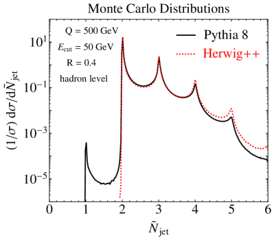
(a)

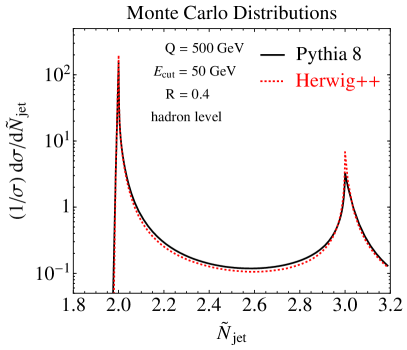
(b)

Figure 1: The $\widetilde{N}_{\rm jet}$ distribution in $e^{+}e^{-}$ collisions from Pythia 8 and Herwig++, over a wide range of multiplicities (left plot) and for $2\lesssim\widetilde{N}_{\rm jet}\lesssim 3$ (right plot). The distribution peaks at integer values, and near-integer values are enhanced relative to intermediate values between integers. It is this enhancement that we will understand quantitatively through our calculations.

The $\widetilde{N}_{\rm jet}$ distribution is peaked at integer values, with substantial support in the near-integer regime. These different parts of the $\widetilde{N}_{\rm jet}$ distribution can be qualitatively studied with Monte Carlo generators. We generate events for $e^{+}e^{-}\to$ hadrons at a center-of-mass energy of $Q=500$ GeV in Pythia 8.183 Sjostrand:2007gs and Herwig++ 2.7.1 Bahr:2008pv , including showering and hadronization. In Fig. 1a, we plot the distribution of $\widetilde{N}_{\rm jet}$ across a wide range of values, showing the circus-tent-like peak and fall-off behavior of the cross section. In Fig. 1b, we focus on the distribution in the range $2\lesssim\widetilde{N}_{\rm jet}\lesssim 3$, which is the region we aim to quantitatively describe in this paper. In Fig. 2, we plot the $\widetilde{N}_{\rm jet}$ distribution in a “triptych” form that shows in more detail the near-integer behavior in $\Delta_{2-}$, $\Delta_{2+}$, and $\Delta_{3-}$, in particular the logarithmic enhancement as $\Delta_{n\pm}\to 0$.

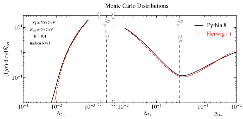
Figure 2: The same $\widetilde{N}_{\rm jet}$ distributions as Fig. 1, now plotted in “triptych” form to show the near-integer behavior in $\Delta_{2-}$, $\Delta_{2+}$, and $\Delta_{3-}$. Note that the $\Delta_{2-}$ and $\Delta_{3-}$ axes run backwards. The $\Delta_{2-}$ and $\Delta_{2+}$ distributions interface at $\widetilde{N}_{\rm jet}=2$ (where $\Delta_{2\pm}=0$), indicated by the left-hand dashed vertical line. Since we do not plot $\Delta_{2\pm}$ all the way to 0, we put a gap over the region around $\widetilde{N}_{\rm jet}=2$. The $\Delta_{2+}$ and $\Delta_{3-}$ distributions are connected at $\widetilde{N}_{\rm jet}=2.5$ (where $\Delta_{2+}=\Delta_{3-}=0.5$), indicated by the right-hand dashed vertical line.

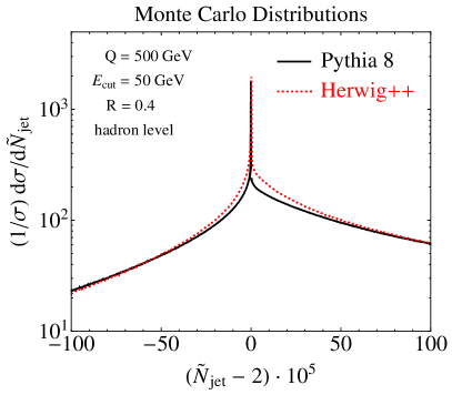
(a)

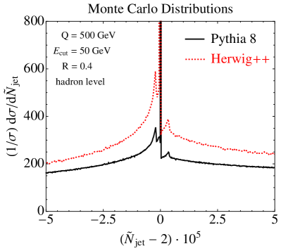
(b)

Figure 3: The same $\widetilde{N}_{\rm jet}$ distributions as Fig. 1, now plotted in the very near vicinity of $\widetilde{N}_{\rm jet}=2$. Note the scale on the $x$-axis and the fact that the $y$-axis is logarithmic on the left plot but linear on the right one. At $\widetilde{N}_{\rm jet}=2$, there is a spike in the distribution from the jet algorithm behavior of the fractional jet multiplicity. At non-integer values, the continuous distribution is more similar to event shapes. We show the near-integer values in two different ranges, and for the closer range (right plot) one can see bumps in the Monte Carlo distributions from multiple emission and hadronization effects.

As mentioned in the introduction, the cross section at exact integer values has a different behavior than at near-integer values, a feature related to the hybrid jet algorithm/event shape nature of the observable. Like a jet algorithm, the cross section at integer values $\widetilde{N}_{\rm jet}=n$ has a non-zero value. Like an event shape, the non-integer cross section is suppressed by all-orders emissions as $\widetilde{N}_{\rm jet}\to n$. The behavior can be seen in Fig. 3, where we plot the distribution in the very near vicinity of $\widetilde{N}_{\rm jet}=2$.

The reason why integer values $\widetilde{N}_{\rm jet}=n$ have a finite cross section is that they receive contributions from regions of phase space with non-zero measure. This can be seen easily at $\mathcal{O}\!\left(\alpha_{s}\right)$ for $e^{+}e^{-}\to q\overline{q}g$, where the entire cross section lies at $\widetilde{N}_{\rm jet}=2$ or $3$. More generally, any collection of particles within a mutual radius of $R$ will give an integer contribution to $\widetilde{N}_{\rm jet}$. This means that the differential distribution at integer values has the form

$$\frac{\text{d}\sigma}{\text{d}\widetilde{N}_{\rm jet}}(\widetilde{N}_{\rm jet}=n)\propto\delta(n)\,.$$ (6)

In contrast, the distribution for near-integer values $\Delta_{n\pm}>0$ is dominated by logarithms of $\Delta_{n\pm}$. We will later show that the logarithms of $\Delta_{n\pm}$ arise from soft emissions, and the most important terms scale single logarithmically as $(\alpha_{s}\ln\Delta_{n\pm})^{k}$. These logarithms combine at all orders to suppress the cross section as $\Delta_{n\pm}\to 0$, leading to the disjoint behavior at integer $\widetilde{N}_{\rm jet}$. Note that single-logarithmic suppression is not as strong as the more familiar double-logarithmic suppression, so there are no Sudakov peaks in the $\Delta_{n\pm}$ distributions.

2.2 Soft and Collinear Limits of Fractional Jets

To understand the leading near-integer behavior of $\widetilde{N}_{\rm jet}$, we can focus on the soft and collinear limits. As discussed further in Sec. 5, the all-orders structure of the cross section does not satisfy standard soft-collinear factorization, but a soft-collinear analysis is still fruitful at fixed order. The essential physics appears already in the three-parton phase space, where the near-integer behavior is dominated by soft physics. We will focus on a single jet region here; to describe $e^{+}e^{-}\to\text{dijets}$, we sum over the contributions to $\widetilde{N}_{\rm jet}$ from both jet regions (see Eq. (61)).

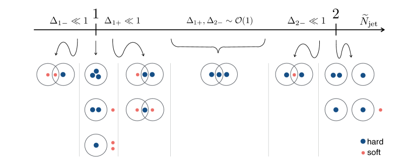
Figure 4: Schematic representation of the different phase space configurations with three merged partons. The numbered line shows the corresponding range of $\widetilde{N}_{\rm jet}$. Here, we are considering just a single jet region; an $e^{+}e^{-}\to\text{dijet}$ event has two such jet regions. Circles represent cones of radius $R$, large blue dots represent energetic partons, and small red dots represent soft partons with $z<z_{\text{cut}}$. The near-integer regions $\Delta_{1-}$, $\Delta_{1+}$, and $\Delta_{2-}$ get contributions from single- and/or double-soft emissions.

We call a group of particles merged if their contribution to $\widetilde{N}_{\rm jet}$ is connected, such that removing a subset of particles affects the contribution to $\widetilde{N}_{\rm jet}$ from other particles. For a single isolated particle, its contribution to $\widetilde{N}_{\rm jet}$ is 1. For a merged pair of particles with separation less than $R$, one still obtains an integer value of $\widetilde{N}_{\rm jet}$:

$$\widetilde{N}_{\rm jet}=\frac{E_{1}}{E_{1}+E_{2}}+\frac{E_{2}}{E_{1}+E_{2}}=1.$$ (7)

Because a single soft/collinear emission does not contribute to the value of $\widetilde{N}_{\rm jet}$, it is not linear in soft and collinear momenta in the singular region of phase space, and hence it is a non-additive observable.

Now consider three merged partons. As shown in Fig. 4, there are various different phase space configurations that lead to different values of $\widetilde{N}_{\rm jet}$. To achieve non-integer values, one needs a phase space configuration with

$$\theta_{12}>R\,,\qquad\theta_{13},\theta_{23}<R,$$ (8)

or permutations of the parton labels. If all $E_{i}>E_{{\rm cut}}$, then the contribution to the jet multiplicity is

$$\widetilde{N}_{\rm jet}=\frac{E_{1}}{E_{1}+E_{3}}+\frac{E_{2}}{E_{2}+E_{3}}+\frac{E_{3}}{E_{1}+E_{2}+E_{3}}\in(1,2)\,.$$ (9)

In terms of energy fractions

$$z_{i}\equiv\frac{E_{i}}{E_{1}+E_{2}+E_{3}}\,,\qquad z_{1}+z_{2}+z_{3}=1\,,\qquad z_{\rm cut}\equiv\frac{E_{{\rm cut}}}{E_{1}+E_{2}+E_{3}}\,,$$ (10)

which removes the overall energy scale of the jet as a degree of freedom, the observable takes the value

$$\widetilde{N}_{\rm jet}=\frac{z_{1}}{z_{1}+z_{3}}+\frac{z_{2}}{z_{2}+z_{3}}+z_{3}\,.$$ (11)

For this merged triplet, near-integer behavior is obtained when one or two of the partons goes soft, as shown in Fig. 4. In these soft limits, the observable may depend on a single soft momentum or a product of soft momenta. For example, if particle 1 is soft,

$$\widetilde{N}_{\rm jet}\xrightarrow[\;z_{1}\,\ll\,1\;]{}\;1+z_{1}\frac{z_{2}(2-z_{2})}{1-z_{2}}+\mathcal{O}\!\left(z_{1}^{2}\right)\,.$$ (12)

Or, if particles 1 and 2 are both soft,

$$\widetilde{N}_{\rm jet}\xrightarrow[\;z_{1,2}\,\ll\,1\;]{}\;1+2z_{1}z_{2}+\mathcal{O}\!\left(z_{1,2}^{3}\right)\,.$$ (13)

The first case is typical of event shape observables, as the near-integer behavior is linear in the soft particle’s energy. The second case, however, is unusual—it goes as the product of soft momenta, another demonstration of the non-additive nature of $\widetilde{N}_{\rm jet}$. This feature creates a novel structure in the perturbative series, reminiscent of rapidity divergences in SCET_II Chiu:2009yx ; Chiu:2011qc . We discuss this further in Sec. 3, using a toy observable $\Delta=z_{1}z_{2}$ that exhibits the same analytic features.

With more emissions, near-integer behavior requires the soft limit of one or more particles. As mentioned above, an arbitrary collection of energetic particles will yield an integer $\widetilde{N}_{\rm jet}$ if the particles can be grouped into merged clusters where each particle in the cluster is within $R$ of all other particles in the cluster (such that each cluster has $\widetilde{N}_{\rm jet}=1$). Non-integer values are obtained when this is not satisfied (as in the merged triplet example above), though generically the resulting values are far from integers. Near-integer values are obtained by starting from an integer $\widetilde{N}_{\rm jet}$ configuration and then adding any number of soft particles which are not within the mutual radius $R$ of the cluster. The contribution of these soft particles to $\widetilde{N}_{\rm jet}$ will be suppressed by

$$\frac{E_{\rm soft}}{E_{{\rm soft},R}}\,,$$ (14)

and the deviation of $\widetilde{N}_{\rm jet}$ from integer values is similarly suppressed by this ratio as long as $E_{{\rm soft},R}>E_{\text{cut}}$. In this way, the near-integer behavior is determined by soft emissions in the vicinity of hard clusters, and soft emissions will generate logarithms of $\Delta_{n\pm}$.

By contrast, collinear splittings cannot generate near-integer behavior of $\widetilde{N}_{\rm jet}$ and hence do not generate logarithms of $\Delta_{n\pm}$. For collinear splittings of angle $R_{c}$, the only effect on $\widetilde{N}_{\rm jet}$ comes from particles who are within $R$ of either of the two daughters or the parent, but not within $R$ of all three. For small $R_{c}$, this is a power-suppressed region of phase space and not logarithmically enhanced. Said another way, the effect on $\widetilde{N}_{\rm jet}$ from a small-angle splitting is not smooth, as it either preserves the value of $\widetilde{N}_{\rm jet}$ or discretely changes it by including or excluding particles from the various $E_{i,R}$ terms; this behavior cannot generate logarithms of $\Delta_{n\pm}$. So unlike standard jet shapes (like jet mass) which depend on both the softness and collinearity of a splitting, the near-integer $\widetilde{N}_{\rm jet}$ value depends only on the softness of emissions.

2.3 Non-Global yet Local Structure

We have argued that soft emissions contribute to near-integer values of $\widetilde{N}_{\rm jet}$, but this is only the case if the soft emissions lie within a restricted phase space of size $\lesssim 2R$ around the jet. Wide-angle soft radiation does not contribute to $\widetilde{N}_{\rm jet}$, since those emissions yield $E_{i,R}<E_{{\rm cut}}$. This angular restriction on soft radiation produces non-global logarithms of $\Delta_{n\pm}$, which are logarithms that arise from emissions in a restricted angular region of phase space Dasgupta:2001sh ; Dasgupta:2002bw .

At leading order, non-global logarithms are often associated with correlated soft emissions from non-Abelian matrix elements and are therefore proportional to $C_{F}C_{A}$. For the case of fractional jet multiplicity, however, the measurement itself introduces a correlation between different emissions, and this effect appears for both non-Abelian and Abelian matrix elements. As we discuss in detail in Sec. 4.1, the allowed phase space for a soft emission to change $\widetilde{N}_{\rm jet}$ depends on the phase space of other soft emissions and on the phase space of the hard partons, similarly to what happens for clustering logarithms Banfi:2005gj ; Delenda:2006nf ; KhelifaKerfa:2011zu ; Kelley:2012kj . In this regard, all soft logarithms of $\widetilde{N}_{\rm jet}$, including those proportional to $C_{F}^{2}$, can be considered non-global.

Moreover, the fact that the allowed phase space for soft emissions to change $\widetilde{N}_{\rm jet}$ depends on the phase space of the hard partons means that one cannot consider how $\widetilde{N}_{\rm jet}$ depends on soft emissions without also considering collinear emissions, and vice versa. Because the contributions to $\widetilde{N}_{\rm jet}$ from soft and collinear emissions are inextricably linked, we will show in Sec. 5.2 that $\widetilde{N}_{\rm jet}$ does not obey standard soft-collinear factorization Bauer:2001yt ; Bauer:2008jx ; Ellis:2010rwa ; Walsh:2011fz . As mentioned above, collinear emissions by themselves do not generate logarithms of $\widetilde{N}_{\rm jet}$, but they do alter the allowed phase space for soft radiation within a jet region. Thus, collinear emissions will modify the coefficients of soft logarithms of $\widetilde{N}_{\rm jet}$, which is a sign of collinear-soft non-factorization.

While the $\Delta_{n\pm}$ dependence is non-global, it is also local to each jet. Emissions affecting $\widetilde{N}_{\rm jet}$ are restricted to an angular region of $\lesssim 2R$ around each jet direction. Additional emissions away from all jets can also create their own jets, changing $\widetilde{N}_{\rm jet}$ by an integer or near-integer amount, but an emission far from all jets cannot change $\widetilde{N}_{\rm jet}$ by a small amount. Because of color coherence, this implies that the contribution to $\widetilde{N}_{\rm jet}$ from a given jet is, to leading power, independent of all other jets in the event. The $\widetilde{N}_{\rm jet}$ distribution is therefore a sum of contributions from jet regions that are to a good approximation independently determined. We will formalize this “local” factorization structure in Sec. 5.4, and see how it could simplify LHC calculations in Sec. 6.

3 Rapidity-like Divergences

As mentioned in Sec. 2.2, the calculation of $\widetilde{N}_{\rm jet}$ at $\mathcal{O}(\alpha_{s}^{2})$ features divergences not regulated by dimensional regularization (dim reg) when the calculation is divided into unique soft limits. These divergences have a strong resemblance to rapidity divergences in SCET_II, where the large rapidities of soft and collinear modes in the effective theory generate divergent integrals not regulated by dim reg Chiu:2009yx ; Chiu:2011qc ; Chiu:2012ir . The similar divergences appearing in the $\widetilde{N}_{\rm jet}$ calculation are not from physical rapidities, but instead originate from the energy sharing between particles and are easily cast in terms of a “rapidity” of this energy sharing:

$$y=\frac{1}{2}\ln\frac{z_{1}}{z_{2}}\,.$$ (15)

In this section, we show how these divergences arise in the $\widetilde{N}_{\rm jet}$ calculation and how we can adapt standard rapidity regulators to our case.

Instead of the complete $\widetilde{N}_{\rm jet}$ calculation, consider the simplified observable

$$\Delta=z_{1}z_{2}\,,$$ (16)

where particles 1 and 2 are particles that may be soft. $\Delta$ has the same soft scaling properties as the near-integer behavior of $\widetilde{N}_{\rm jet}$ (see Eqs. (12) and (13)), and the other complications from the complete $\widetilde{N}_{\rm jet}$ calculation are irrelevant for the discussion here. Like $\Delta_{2+}$ to be calculated in Sec. 4.1, $\Delta$ receives contributions from both single-soft and double-soft regions of phase space. Also like $\Delta_{2+}$, $\Delta$ is a non-additive observable that does not get a linear contribution from each soft emission.

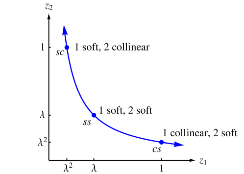
Figure 5: The single- and double-soft modes depicted in the $z_{1}$-$z_{2}$ plane for the simplified observable $\Delta=z_{1}z_{2}$ (similar to $\Delta_{2+}$). We assign the power counting $\Delta\sim\lambda^{2}$. In the case with only one soft particle, the soft energy scales as $\lambda^{2}$, whereas in the case with two soft particles, the soft energies scale as $\lambda$. These modes are connected by the hyperbola shown, which can be thought of as tracing out the rapidity in the energies of the two partons (see Eq. (15)). In our calculation, we encounter divergences in this rapidity variable for each mode depicted. This picture has a strong analog in the divergences in physical rapidity of single particles in SCET_II.

The interplay between the single- and double-soft limits is illustrated in Fig. 5. In order to have a consistent power counting for $\Delta$, we need to consider two different scalings of the soft modes. Let $\lambda\ll 1$ be the power counting parameter, with $\Delta\sim\lambda^{2}$. The phase space regions with the same parametric contribution to $\Delta$ are:

1 soft, 2 collinear ($$sc z_{1}\sim\lambda^{2}\,,\;z_{2}\sim 1\,,$$):

1 soft, 2 soft ($$ss z_{1}\sim\lambda\,,\;z_{2}\sim\lambda\,,$$):

1 collinear, 2 soft ($$cs z_{1}\sim 1\,,\;z_{2}\sim\lambda^{2}\,.$$): (17)

Thus, there are two types of soft modes — single-soft modes scale as $\lambda^{2}$, whereas double-soft modes scale as $\lambda$ — and there is a unique soft power counting within each sector. This relative scaling is the same as ultrasoft modes in SCET_I (which scale as $\lambda^{2}$) and soft modes in SCET_II (which scale as $\lambda$). This indicates that the calculation has contributions to the observable from soft modes in both SCET_I and SCET_II. The “energy rapidity” variable $y$ in Eq. (15) separates these phase space regions by measuring the relative energy sharing between particles 1 and 2. Like an ordinary rapidity, the range is $y\in(-\infty,\infty)$. The $sc$ region has $z_{1}\ll z_{2}$ ($y\to-\infty$), the $ss$ region has $z_{1}\simeq z_{2}$ ($\lvert y\rvert\simeq 1$), and the $cs$ region has $z_{1}\gg z_{2}$ ($y\to\infty$). Each of the $sc$/$cs$/$ss$ sectors gives an independent contribution to the $\Delta$ distribution at $\mathcal{O}(\alpha_{s}^{2})$ which should be properly summed (i.e. one has to remove potential double-counting). As we will now see, unbounded integrals in $y$ produce divergences, not regulated by dim reg.

In full QCD with dim reg in $d=4-2\epsilon$ dimensions, the soft divergences of $\Delta$ are encapsulated by the integral

$$I_{\rm full}(\Delta) =\int_{0}^{1}\frac{\text{d}z_{1}}{z_{1}}\frac{\text{d}z_{2}}{z_{2}}\,(z_{1}z_{2})^{-2\epsilon}\,\delta(\Delta-z_{1}z_{2})$$

$$=\Delta^{-1-2\epsilon}\int_{-\infty}^{\infty}\text{d}y\,\Theta\Bigl{(}-\frac{1}{2}\ln(1/\Delta)<y<\frac{1}{2}\ln(1/\Delta)\Bigr{)}$$

$$=\frac{1}{4\epsilon^{2}}\delta(\Delta)-\mathcal{L}_{1}(\Delta)\,\Theta(\Delta<1)+\mathcal{O}\!\left(\epsilon\right)\,,$$ (18)

where $\mathcal{L}_{1}$ is a logarithmic plus-function defined in Eq. (91). If we take soft limits of the phase space, where the boundaries scale as $[0,1]\to[0,\infty]$, we get:

$$\text{1 soft: }\;I_{sc}(\Delta) =\int_{0}^{\infty}\frac{\text{d}z_{1}}{z_{1}}\int_{0}^{1}\frac{\text{d}z_{2}}{z_{2}}\,(z_{1}z_{2})^{-2\epsilon}\,\delta(\Delta-z_{1}z_{2})$$

$$=\Delta^{-1-2\epsilon}\int_{-\infty}^{\infty}\text{d}y\,\Theta\Bigl{(}-\frac{1}{2}\ln(1/\Delta)<y\Bigr{)}\,,$$

$$\text{2 soft: }\;I_{cs}(\Delta) =\int_{0}^{1}\frac{\text{d}z_{1}}{z_{1}}\int_{0}^{\infty}\frac{\text{d}z_{2}}{z_{2}}\,(z_{1}z_{2})^{-2\epsilon}\,\delta(\Delta-z_{1}z_{2})$$

$$=\Delta^{-1-2\epsilon}\int_{-\infty}^{\infty}\text{d}y\,\Theta\Bigl{(}y<\frac{1}{2}\ln(1/\Delta)\Bigr{)}\,,$$

$$\text{1, 2 soft: }\;I_{ss}(\Delta) =\int_{0}^{\infty}\frac{\text{d}z_{1}}{z_{1}}\int_{0}^{\infty}\frac{\text{d}z_{2}}{z_{2}}\,(z_{1}z_{2})^{-2\epsilon}\,\delta(\Delta-z_{1}z_{2})$$

$$=\Delta^{-1-2\epsilon}\int_{-\infty}^{\infty}\text{d}y\,.$$ (19)

Each integral is divergent and unregulated, but the $\Delta<1$ regime of full QCD is reproduced by the combination

$$I_{\rm full}(\Delta)=\bigl{[}I_{sc}(\Delta)+I_{cs}(\Delta)-I_{ss}(\Delta)\bigr{]}\Theta(\Delta<1).$$ (20)

This result is as expected, since the double-soft limit should remove the double-counting of the single-soft limits, even if each contribution is not well-defined individually. Note that the unregulated divergences appear only in $y$.

This structure of divergences in $y$ is identical to those in physical rapidities of single particles in SCET_II. These divergences may be handled in a number of ways, and we will use the rapidity renormalization group (rapidity RG) Chiu:2011qc ; Chiu:2012ir . In the rapidity RG, divergences are regulated analogously to dim reg, using a scale $\nu$ and infinitesimal parameter $\eta$ that correspond to the usual $\mu$ and $\epsilon$ in dim reg. At one loop, these regulator factors are Chiu:2011qc ; Chiu:2012ir

$$\text{1 soft: }\;R^{sc}_{\eta} =\Bigl{(}\frac{\nu}{E_{J}}\Bigr{)}^{\eta}z_{2}^{-\eta}=\Bigl{(}\frac{\nu}{E_{J}}\Bigr{)}^{\eta}s^{-\eta/2}e^{y\eta}\,,$$

$$\text{2 soft: }\;R^{cs}_{\eta} =\Bigl{(}\frac{\nu}{E_{J}}\Bigr{)}^{\eta}z_{1}^{-\eta}=\Bigl{(}\frac{\nu}{E_{J}}\Bigr{)}^{\eta}s^{-\eta/2}e^{-y\eta}\,,$$

$$\text{1, 2 soft: }\;R^{ss}_{\eta} =\Bigl{(}\frac{\nu}{E_{J}}\Bigr{)}^{\eta}\lvert z_{1}-z_{2}\rvert^{-\eta}=\Bigl{(}\frac{\nu}{E_{J}}\Bigr{)}^{\eta}s^{-\eta/2}\lvert 2\sinh y\rvert^{-\eta}\,,$$ (21)

where $s=z_{1}z_{2}$, and $E_{J}$ is the total jet energy such that $z_{i}=E_{i}/E_{J}$. These regulators give well-defined terms for each soft limit,

$$\text{1 soft: }\;I_{sc}(\Delta) =\int_{0}^{\infty}\frac{\text{d}z_{1}}{z_{1}}\int_{0}^{1}\frac{\text{d}z_{2}}{z_{2}}\,(z_{1}z_{2})^{-2\epsilon}\,\delta(\Delta-z_{1}z_{2})\,R^{sc}_{\eta}$$

$$=-\Bigl{(}\frac{\nu}{E_{J}}\Bigr{)}^{\eta}\Delta^{-1-2\epsilon}\,\frac{1}{\eta}\,,$$

$$\text{2 soft: }\;I_{cs}(\Delta) =\int_{0}^{1}\frac{\text{d}z_{1}}{z_{1}}\int_{0}^{\infty}\frac{\text{d}z_{2}}{z_{2}}\,(z_{1}z_{2})^{-2\epsilon}\,\delta(\Delta-z_{1}z_{2})\,R^{cs}_{\eta}$$

$$=-\Bigl{(}\frac{\nu}{E_{J}}\Bigr{)}^{\eta}\Delta^{-1-2\epsilon}\,\frac{1}{\eta}\,,$$

$$\text{1, 2 soft: }\;I_{ss}(\Delta) =\int_{0}^{\infty}\frac{\text{d}z_{1}}{z_{1}}\int_{0}^{\infty}\frac{\text{d}z_{2}}{z_{2}}\,(z_{1}z_{2})^{-2\epsilon}\,\delta(\Delta-z_{1}z_{2})\,R^{ss}_{\eta}$$

$$=\Bigl{(}\frac{\nu}{E_{J}}\Bigr{)}^{\eta}\Delta^{-1-2\epsilon-\eta/2}\biggl{[}\frac{2}{\eta}+\mathcal{O}\!\left(\eta\right)\biggr{]}\,.$$ (22)

Now the sum of contributions is independent of the rapidity regulator and matches the full QCD results for $\Delta<1$:

$$\bigl{[}I_{sc}(\Delta)+I_{cs}(\Delta)+I_{ss}(\Delta)\bigr{]}\Theta(\Delta<1)=\frac{1}{4\epsilon^{2}}\delta(\Delta)-\mathcal{L}_{1}(\Delta)\,\Theta(\Delta<1)+\mathcal{O}\!\left(\epsilon,\eta\right)=I_{\rm full}(\Delta)\,.$$ (23)

Comparing Eq. (23) to Eq. (20), we see that with the rapidity regulator, the full result is reproduced by the sum of single- and double-soft contributions, instead of the difference. This happens because the single- and double-soft limits produce canceling poles in the large positive and negative rapidity regions. For example, the large rapidity limit is allowed in both the $sc$ and $ss$ contributions, where the rapidity regulators scale as

$$\text{1 soft: }\;R^{sc}_{\eta}(y\to\infty) \sim e^{y\eta}\,,$$

$$\text{1, 2 soft: }\;R^{ss}_{\eta}(y\to\infty) \sim e^{-y\eta}\,,$$ (24)

which lead to canceling poles:

1 soft: $$\;\int_{0}^{\infty}\text{d}y\,e^{y\eta}=-\frac{1}{\eta}\,,$$

1, 2 soft: $$\;\int_{0}^{\infty}\text{d}y\,e^{-y\eta}=\frac{1}{\eta}\,.$$ (25)

Thus the cancellation of the large rapidity regimes happens at the level of the sum of contributions, instead of the difference.

Not only does the rapidity RG make the various soft contributions well defined, but it also separates the double-soft limit from the zero-bin subtraction (needed to remove double counting Manohar:2006nz ) of the single-soft limits. Because the rapidity regulators in the single- and double-soft limits are not related by scaling in rapidities, the double-soft contribution is not the zero-bin of the single-soft limit. In fact, the zero-bin limit is scaleless; the rapidity regulator is unchanged in the zero-bin limit but now all rapidities are allowed, leading to the scaleless integral Chiu:2012ir

$$\int_{-\infty}^{\infty}\text{d}y\,e^{\pm y\eta}=0\,.$$ (26)

In SCET_II applications where the collinear and soft contributions to the distribution can be factorized into separated jet/beam and soft functions, this factorization allows these rapidity divergences to be divided into the collinear and soft functions and the resulting logarithms to be resummed using standard techniques (see, e.g., Chiu:2011qc ; Chiu:2012ir ).

The features of rapidity divergences in this simple example of $\Delta$ repeat themselves in the calculation of near-integer behavior of $\widetilde{N}_{\rm jet}$ (specifically, $\Delta_{2+}$) in Sec. 4.1 below.

4 Calculating the Near-Integer Behavior

As seen in Fig. 4, fractional values of $\widetilde{N}_{\rm jet}$ arise when radiation in a jet region extends beyond a radius $R$. In particular, near-integer values of $\widetilde{N}_{\rm jet}$ come from soft radiation beyond $R$, and the deviation from integer values grows as emissions become harder. In this section, we study the leading-order near-integer behavior of $\widetilde{N}_{\rm jet}$ in $e^{+}e^{-}\to\text{jets}$ at a center-of-mass energy of $Q$, which first occurs for $e^{+}e^{-}\to 4$ partons.

Let $\Delta_{2\pm}$ be the jet multiplicity near the 2-jet peak as defined in Eq. (5); we take the power counting $\Delta_{2\pm}\sim\lambda^{2}$, with $\lambda\ll 1$. We will first derive an analytic expression for the cross section at leading order in $\lambda$ (i.e. the singular contributions), including a discussion of the aforementioned rapidity-like divergences. We will then calculate the full $\mathcal{O}\!\left(\alpha_{s}^{2}\right)$ result using the Monte Carlo program Event2 Catani:1996jh ; Catani:1996vz , which allows us to include non-singular terms as well as cross check our results for the singular contributions. We will also calculate the $\mathcal{O}\!\left(\alpha_{s}^{2}\right)$ contributions to $\Delta_{3-}$, though this is not the focus of our studies.

4.1 Singular Contributions using Splitting Functions

The cross section for $\Delta_{2\pm}$ can be written as

$$\frac{\text{d}\sigma}{\text{d}\Delta_{2\pm}}=\int\text{d}\Phi_{4}\,\mathcal{T}(e^{+}e^{-}\to 4\,\text{ partons})\,\mathcal{F}(\Delta_{2\pm},\Phi_{4}),$$ (27)

where $\Phi_{4}$ represents four-body phase space, $\mathcal{T}$ is the matrix element for $e^{+}e^{-}\to 4\text{ partons}$, and $\mathcal{F}(\Delta_{2\pm},\Phi_{4})$ is the measurement function, which projects out the slice of phase space corresponding to a constant value of $\Delta_{2\pm}$. The allowed values of $\widetilde{N}_{\rm jet}$ for four partons are:

Four isolated partons: $$\widetilde{N}_{\rm jet}=4,$$ (28)

Two isolated partons and one merged pair: $$\widetilde{N}_{\rm jet}=3,$$ (29)

One isolated parton and one merged triplet: $$\widetilde{N}_{\rm jet}\in\left(2-(E_{{\rm cut}}/Q)^{2},3\right),$$ (30)

Two merged pairs: $$\widetilde{N}_{\rm jet}=2.$$ (31)

The only non-integer behavior is obtained for the merged triplet in Eq. (30), which requires three particles to be within an angular distance $\lesssim 2R$. Thus, for sufficiently small $R$, we can use the matrix element in the limit where three partons are collinear, allowing us to take advantage of collinear factorization Ellis:1978sf ; Ellis:1978ty ; Catani:1996jh ; Catani:1996vz ; Campbell:1997hg :

$$\mathcal{T}(e^{+}e^{-}\to 4\,\text{ partons}) \simeq\mathcal{T}(e^{+}e^{-}\to q\bar{q})\cdot\sum_{k}\mathcal{T}_{k}^{\text{coll}}(1\to 3)$$ (32)

$$=\mathcal{T}(e^{+}e^{-}\to q\bar{q})\cdot\frac{(8\pi\alpha_{s}\mu^{2\epsilon})^{2}}{s_{123}^{2}}\sum_{k}\langle\hat{P}^{k}_{1\to 3}\rangle\,,$$ (33)

where $k$ labels one of the parton channels $q\to ggq\,,\bar{q}\to gg\bar{q}\,,q\to q^{\prime}\bar{q}^{\prime}q\,,\text{or }\bar{q}\to q^{\prime}\bar{q}^{\prime}\bar{q}$, $s_{123}$ is the squared invariant mass of the three parton system, and $\langle\hat{P}^{k}_{1\to 3}\rangle$ is the spin-averaged $1\to 3$ splitting function Catani:1998nv ; Catani:1999ss . The factorization in Eq. (32) implies that the relevant phase space for the collinear splitting is 3-body, meaning we decompose the 4-body phase space of the whole event into the 2-body $q\bar{q}$ system of the hard interaction and the 3-body phase space of the $1\to 3$ splitting. In the collinear limit, the 4-body phase space factorizes as $\text{d}\Phi_{4}=\text{d}\Phi_{2}(q\bar{q})\times\text{d}s_{123}/(2\pi)\times\text{d}\Phi_{3}(1\to 3)$.

The collinear matrix elements can be further decomposed according to their color structure. The channel $q\to ggq$ (and $\bar{q}\to gg\bar{q}$) can be written as a sum of Abelian (“ab”) and non-Abelian (“nab”) contributions:

$$\mathcal{T}^{\text{coll}}(q\to ggq)=C_{F}^{2}\mathcal{T}_{\rm ab}^{\rm coll}(q\to ggq)+C_{F}C_{A}\mathcal{T}_{\rm nab}^{\rm coll}(q\to ggq),$$ (34)

while the $q\to q^{\prime}\bar{q}^{\prime}q$ (and $\bar{q}\to q^{\prime}\bar{q}^{\prime}\bar{q}$) channels will give contributions proportional to the $C_{F}T_{R}$ color structure. At $\mathcal{O}\!\left(\alpha_{s}^{2}\right)$ the cross section for $\Delta_{2\pm}$ is obtained by summing over all channels and color structures. In the rest of this subsection we will discuss the calculation of the Abelian piece of the cross section; results for the other color structures can be found in App. A.

The Abelian contribution comes from a $q\to ggq$ or $\bar{q}\to gg\bar{q}$ splitting. The two channels give identical contributions and we will focus on the $q\to ggq$ case for definiteness, labeling the final state as:

$$g_{1}g_{2}q_{3}.$$ (35)

As discussed in Sec. 2.2, at leading power we can take the soft limit of our observable, which corresponds to either one or both gluons becoming soft. As in the toy calculation in Sec. 3, we will label the limit where gluon 1 (gluon 2) is soft as $sc$ ($cs$) and the double-soft limit as $ss$. We again use the energy sharing variables $z_{i}=E_{i}/E_{J}$ and scaled veto variable $z_{\rm cut}=E_{\text{cut}}/E_{J}$ in Eq. (10), where here $E_{J}$ is the energy of one jet region (with $E_{J}\simeq Q/2$ for a collision at center-of-mass energy $Q$). We generally assume $z_{\rm cut}\ll 1$, which allows us to neglect power-suppressed contributions from soft quarks, and if some $z_{i}<z_{\rm cut}$ then that particle may be treated as soft.

Observable	$\mathcal{R}_{A}$	$\mathcal{R}_{B}$	$\mathcal{R}_{C}$
$\Delta_{2-}$			–
$\Delta_{2+}$
$\Delta_{3-}$			–

Table 1: Representation of the phase space configurations contributing to the near-integer jet multiplicities $\Delta_{2-}$, $\Delta_{2+}$, and $\Delta_{3-}$. Compared to Fig. 4, the value of $\widetilde{N}_{\rm jet}$ is 1 unit higher, because the event contains an additional isolated parton (not shown). For each observable, we show the corresponding contributions from different angular regions and soft limits. Circles represent cones of radius $R$, large blue dots represent energetic partons, small red dots soft partons with $z<z_{\text{cut}}$. The angular regions $\mathcal{R}_{A}$, $\mathcal{R}_{B}$, and $\mathcal{R}_{C}$ are defined in Eq. (36).

Observable	Region	Expression	Limit	Cuts
$\Delta_{2-}$	$\mathcal{R}_{A}$	$z_{1}z_{2}$	1, 2 soft	$z_{1}+z_{2}<z_{\text{cut}}$
$\Delta_{2-}$	$\mathcal{R}_{B}$	$z_{1}z_{2}$	1, 2 soft	$z_{1}+z_{2}<z_{\text{cut}}$
$\Delta_{2+}$	$\mathcal{R}_{A}$	$z_{1}(1-z_{2}^{2})/z_{2}$	1 soft	$z_{2}>z_{\text{cut}}$
$\Delta_{2+}$	$\mathcal{R}_{B}$	$z_{2}(1-z_{1}^{2})/z_{1}$	2 soft	$z_{1}>z_{\text{cut}}$
$\Delta_{2+}$	$\mathcal{R}_{C}$	$z_{1}z_{2}(2-z_{2})/(1-z_{2})$	1 soft	–
$\Delta_{2+}$	$\mathcal{R}_{C}$	$z_{1}z_{2}(2-z_{1})/(1-z_{1})$	2 soft	–
$\Delta_{2+}$	$\mathcal{R}_{C}$	$2z_{1}z_{2}$	1, 2 soft	–
$\Delta_{3-}$	$\mathcal{R}_{A}$	$z_{2}[1-z_{1}(1-z_{1})]/[z_{1}(1-z_{1})]$	2 soft	$z_{1}>z_{\text{cut}}$
$\Delta_{3-}$	$\mathcal{R}_{B}$	$z_{1}[1-z_{2}(1-z_{2})]/[z_{2}(1-z_{2})]$	1 soft	$z_{2}>z_{\text{cut}}$

Table 2: Near-integer behavior of $\widetilde{N}_{\rm jet}$, shown for various phase space regions as depicted in Table 1. In each case, the expression for the observable is given along with the relevant limits and phase space cuts.

In Tables 1 and 2 we collect contributions to $\Delta_{2\pm}$ in the relevant soft limits and regions of phase space. At this order, we also get a contribution to $\Delta_{3-}=3-\widetilde{N}_{\rm jet}$, and we will carry out the calculation for $\Delta_{3-}$ as well.

We now gather the relevant pieces to evaluate Eq. (27) in the collinear limit. There are three relevant regions of phase space:

$$\mathcal{R}_{A} =\Theta(\theta_{13}>R)\,\Theta(\theta_{23}<R)\,\Theta(\theta_{12}<R),$$ (36)

$$\mathcal{R}_{B} =\mathcal{R}_{A}(1\leftrightarrow 2),$$ (37)

$$\mathcal{R}_{C} =\Theta(\theta_{13}<R)\,\Theta(\theta_{23}<R)\,\Theta(\theta_{12}>R),$$ (38)

where $\theta_{ij}$ labels the opening angle between partons $i$ and $j$. In Table 1 we show a schematic representation of the angular phase space regions and soft limits which are explicitly listed in Table 2. From Table 2, the measurement functions are given by

$$\mathcal{F}(\Delta_{2-},\Phi_{4}) =\mathcal{F}_{\Delta_{2-}}^{\,ss},$$ (39)

$$\mathcal{F}(\Delta_{2+},\Phi_{4}) =\mathcal{F}_{\Delta_{2+}}^{\,sc}+\mathcal{F}_{\Delta_{2+}}^{\,cs}+\mathcal{F}_{\Delta_{2+}}^{\,ss},$$ (40)

$$\mathcal{F}(\Delta_{3-},\Phi_{4}) =\mathcal{F}_{\Delta_{3-}}^{\,sc}+\mathcal{F}_{\Delta_{3-}}^{\,cs},$$ (41)

where

$$\mathcal{F}_{\Delta_{2-}}^{\,ss} =\delta(\Delta_{2-}-z_{1}z_{2})\,\Theta(z_{1}+z_{2}<z_{\text{cut}})\,\mathcal{R}_{A}+(1\leftrightarrow 2),$$ (42)

$$\begin{split}\mathcal{F}_{\Delta_{2+}}^{\,sc}&=\,\delta\left[\Delta_{2+}-z_{1}\left(1/z_{2}-z_{2}\right)\right]\,\Theta(z_{2}>z_{\text{cut}})\mathcal{R}_{A}\\ &\quad+\delta[\Delta_{2+}-z_{1}z_{2}(2-z_{2})/(1-z_{2})]\,\mathcal{R}_{C},\end{split}$$ (43)

$$\mathcal{F}_{\Delta_{2+}}^{\,cs} =\mathcal{F}_{\Delta_{2+}}^{\,sc}(1\leftrightarrow 2),$$ (44)

$$\mathcal{F}_{\Delta_{2+}}^{\,ss} =\delta(\Delta_{2+}-2z_{1}z_{2})\,\mathcal{R}_{C},$$ (45)

$$\mathcal{F}_{\Delta_{3-}}^{\,sc} =\delta\left(\Delta_{3-}-z_{1}[1-z_{2}(1-z_{2})]/[z_{2}(1-z_{2})]\right)\,\Theta(z_{2}>z_{\text{cut}})\mathcal{R}_{B},$$ (46)

$$\mathcal{F}_{\Delta_{3-}}^{\,cs} =\mathcal{F}_{\Delta_{3-}}^{\,sc}(1\leftrightarrow 2).$$ (47)

The single- and double-soft limits for the $1\to 3$ matrix elements are

$$\mathcal{T}_{\rm ab}(q\to g_{1}g_{2}q_{3})\simeq\begin{cases}\mathcal{T}_{\rm ab}^{sc}=\dfrac{4(4\pi\alpha_{s}\mu^{2\epsilon})^{2}}{E_{J}^{4}}\dfrac{2-2z_{2}+z_{2}^{2}(1-\epsilon)}{\theta_{13}^{2}\theta_{23}^{2}z_{1}^{2}z_{2}^{2}(1-z_{2})},&\mbox{(1 soft, 2 collinear)}\vspace{1ex}\\ \mathcal{T}_{\rm ab}^{cs}=\mathcal{T}_{\rm ab}^{sc}(1\leftrightarrow 2),&\mbox{(1 collinear, 2 soft)}\vspace{1ex}\\ \mathcal{T}_{\rm ab}^{ss}=\dfrac{8(4\pi\alpha_{s}\mu^{2\epsilon})^{2}}{E_{J}^{4}}\dfrac{1}{\theta_{13}^{2}\theta_{23}^{2}z_{1}^{2}z_{2}^{2}},&\mbox{(1 soft, 2 soft)}\end{cases}$$ (48)

where we have included a symmetry factor of $1/2!$ for identical gluons. Notice that in the double-soft limit, the Abelian matrix element simply reduces to the product of two eikonal factors. In the collinear regime, the 3-body phase space can be written as GehrmannDeRidder:1997gf

$$\text{d}\Phi_{3}^{\rm coll}=\frac{E_{J}^{4-4\epsilon}}{(4\pi)^{4-2\epsilon}\Gamma(1-2\epsilon)}\,\text{d}\Phi_{\Omega}\,\text{d}\Phi_{z},$$ (49)

where the angular phase space $\text{d}\Phi_{\Omega}$ is given by

$$\text{d}\Phi_{\Omega}=\text{d}\theta_{13}^{2}\text{d}\theta_{23}^{2}\text{d}\theta_{12}^{2}\Theta(\Delta)\Delta^{-1/2-\epsilon},\quad\Delta=4\theta_{13}^{2}\theta_{23}^{2}-(\theta_{12}^{2}-\theta_{23}^{2}-\theta_{13}^{2})^{2},$$ (50)

and the energy phase space $\text{d}\Phi_{z}$ is given by

$$\text{d}\Phi_{z}\simeq\begin{cases}\text{d}\Phi_{z}^{sc}=\Theta(z_{1}<\infty)\Theta(z_{2}<1)[z_{1}z_{2}(1-z_{2})]^{1-2\epsilon}\text{d}z_{1}\text{d}z_{2},&\mbox{(1 soft, 2 collinear)}\\ \text{d}\Phi_{z}^{cs}=\text{d}\Phi_{z}^{sc}(1\leftrightarrow 2),&\mbox{(1 collinear, 2 soft)}\\ \text{d}\Phi_{z}^{ss}=\Theta(z_{1}<\infty)\Theta(z_{2}<\infty)(z_{1}z_{2})^{1-2\epsilon}\text{d}z_{1}\text{d}z_{2}.&\mbox{(1 soft, 2 soft)}\end{cases}$$ (51)

As discussed in Sec. 3, for certain contributions to the observable, these energy integrals give rise to rapidity divergences which require special regularization to make each term well defined. We use the rapidity regulator to do this, and the sum of all contributions is regulator independent. Specifically, the contribution to $\Delta_{2+}$ from $\mathcal{R}_{C}$ is the only one with both single- and double-soft limits (see Tables 1 and 2), and hence the only contribution which requires this extra regulator. While $\Delta_{2-}$ does receive contributions from the double-soft region of phase space, the constraints on the gluon energies from $z_{\rm cut}$ implies that both gluons must be soft, and hence the single-soft limits do not contribute. The limit on the gluon energies also implies there is a kinematic limit on the observable, $\Delta_{2-}<(z_{\rm cut}/2)^{2}$.

By combining the measurement function with the proper limits of the matrix elements, we get an analytic expression for the Abelian contribution to the $\Delta_{2\pm}$ and $\Delta_{3-}$ distributions at leading power in $\lambda$. Including the identical contribution from $\bar{q}\to\bar{q}gg$ yields

$$\left[\frac{\text{d}\sigma}{\text{d}\Delta_{2-}}\right]_{\rm ab} =C_{F}^{2}\left(\frac{\alpha_{s}}{\pi}\right)^{2}\mathcal{I}_{\Omega}\bigl{\{}-2\mathcal{L}_{1}(\Delta_{2-})+4\ln z_{\text{cut}}\,\mathcal{L}_{0}(\Delta_{2-})\bigr{\}}\Theta(\Delta_{2-}<z_{\rm cut}^{2}/4)\,,$$ (52)

$$\left[\frac{\text{d}\sigma}{\text{d}\Delta_{2+}}\right]_{\rm ab} =C_{F}^{2}\left(\frac{\alpha_{s}}{\pi}\right)^{2}\mathcal{I}_{\Omega}\biggl{\{}-\frac{14}{5}\mathcal{L}_{1}(\Delta_{2+})+\biggl{(}-\frac{57}{10}+\frac{14}{5}\ln 2-2\ln z_{\text{cut}}\biggr{)}\mathcal{L}_{0}(\Delta_{2+})\biggr{\}}\,,$$ (53)

$$\left[\frac{\text{d}\sigma}{\text{d}\Delta_{3-}}\right]_{\rm ab} =C_{F}^{2}\left(\frac{\alpha_{s}}{\pi}\right)^{2}\mathcal{I}_{\Omega}\biggl{(}-\frac{3}{2}-2\ln z_{\text{cut}}\biggr{)}\mathcal{L}_{0}(\Delta_{3-})\,,$$ (54)

where the distributions $\mathcal{L}_{n}$ are the usual logarithmic plus distributions, defined in App. B. The integral over the angular phase space is given by

$$\mathcal{I}_{\Omega}=\frac{4}{\pi}\int\frac{\text{d}\Phi_{\Omega}}{\theta_{13}^{2}\theta_{23}^{2}}\mathcal{R}_{A}=\frac{5\pi^{2}}{54}\,.$$ (55)

Eqs. (52), (53), and (54) represent the leading order distributions in the small $R$ and $z_{\text{cut}}$ limits. Notice that at this order there is no dependence on $R$, as the $1/\theta_{ij}^{2}$ factors in the denominator of the angular integral provide a logarithmic scaling which can be used to explicitly remove the $R$ dependence. Since we are focused on the non-integer behavior of $\widetilde{N}_{\rm jet}$, we have suppressed contributions proportional to $\delta(\Delta_{n\pm})$ in our results (see, however, Eq. (64)).

The calculation of the $C_{F}C_{A}$ and $C_{F}T_{R}n_{f}$ contributions are very similar to the Abelian case, albeit more involved as the matrix elements do not simply factorize into separate angular and energy functions as in Eq. (48). In App. A, we give the full set of results for the different color structures.

In the $\mathcal{O}\!\left(\alpha_{s}^{2}\right)$ calculation performed above, double logarithms of $\Delta_{n\pm}$ (appearing as $\mathcal{L}_{1}(\Delta_{n\pm})$) arose when both emitted gluons became soft, and single logarithms ($\mathcal{L}_{0}(\Delta_{n\pm})$) arose when a single gluon became soft. This correspondence holds true with more soft emissions: each soft emission results in a single logarithm of $\Delta_{n\pm}$ (in certain regions of phase space). Therefore, in general the largest logarithm at $\mathcal{O}\!\left(\alpha_{s}^{k}\right)$ appears when all emissions are soft gluons, and the contribution to the cross section is of the form $\alpha_{s}^{k}\mathcal{L}_{k-1}(\Delta_{n\pm})$.

4.2 Nonsingular Contributions from Event2

To go beyond leading power in $\lambda$, we need to incorporate the $\mathcal{O}\!\left(\alpha_{s}^{2}\right)$ matrix elements from full QCD. For fixed-order calculations of $e^{+}e^{-}\to\text{partons}$ at low multiplicity, the program Event2 is a particularly useful tool Catani:1996jh ; Catani:1996vz . Event2 performs next-to-leading order calculations of $e^{+}e^{-}\to$ 2 and 3 partons, so it includes the needed $e^{+}e^{-}\to 4$ parton tree-level matrix elements. Conveniently, it allows for the decomposition of its results order-by-order in $\alpha_{s}$ and by color structure. Crucially, Event2 can probe the far infrared regions of phase space, meaning the (singular) logarithmic terms of $\Delta_{2\pm}$ and $\Delta_{3-}$ are enhanced. This allows us to perform a robust comparison and cross check of our splitting function calculations above. Having verified the singular logarithmic contributions to $\Delta_{2\pm}$ and $\Delta_{3-}$, we can then extract the nonsingular $\mathcal{O}\!\left(\alpha_{s}^{2}\right)$ contributions directly from Event2.

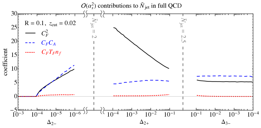
Figure 6: The $\Delta_{2\pm}$ and $\Delta_{3-}$ distributions extracted from Event2. Shown are the separate $C_{F}^{2}$, $C_{F}C_{A}$, and $C_{F}T_{F}n_{f}$ contributions to the cross section, plotted as the coefficient of $(\alpha_{s}/2\pi)^{2}\,C$, where $C$ is the relevant color factor. Note that the $\Delta_{2-}$ and $\Delta_{3-}$ axes run backwards.

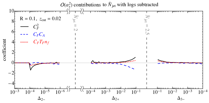
Figure 7: Same as Fig. 6, but subtracting our calculations for the singular contributions in each region. The residuals vanish in the logarithmic ($\Delta_{n\pm}\to 0$) regime, indicating that the only remaining terms are nonsingular.

In Fig. 6, we show the $\mathcal{O}\!\left(\alpha_{s}^{2}\right)$ contributions to $\Delta_{2\pm}$ and $\Delta_{3-}$ extracted from Event2. We plot the coefficients of the $(\alpha_{s}/2\pi)^{2}\,C$ terms in the cross section as a function of $\ln\Delta_{n\pm}$, where $C$ is the relevant color factor ($C_{F}^{2}$, $C_{F}C_{A}$, or $C_{F}T_{F}n_{f}$). To enhance the logarithmic contributions and minimize the power corrections in $R$ and $z_{\rm cut}$, we choose the small values $R=0.1$ and $z_{\rm cut}=0.02$. Plotted this way, double logarithms $\bigl{(}\mathcal{L}_{1}(\Delta_{n\pm})\bigr{)}$ appear as lines of constant non-zero slope, single logarithms $\bigl{(}\mathcal{L}_{0}(\Delta_{n\pm})\bigr{)}$ appear as lines with zero slope and non-zero offset, and nonsingular contributions vanish as $\Delta_{n\pm}\to 0$. It is clear that logarithmically-enhanced terms are indeed present in the full QCD result from Event2.

To make sure the logarithmic behavior from Event2 matches our analytic calculations in Sec. 4.1 and App. A, we can extract the nonsingular contribution to the cross section, which are the residual fixed-order terms after the logarithmic contributions are subtracted:

$$\frac{\text{d}\sigma_{\rm ns}}{\text{d}\Delta_{n\pm}}=\frac{\text{d}\sigma_{\rm full}}{\text{d}\Delta_{n\pm}}-\frac{\text{d}\sigma_{\rm sing}}{\text{d}\Delta_{n\pm}}\,.$$ (56)

These are shown in Fig. 7, again separated by color structure, and confirm that our splitting function calculation, which includes the leading contributions in a small $R$ and $z_{\text{cut}}$ expansion, captures the leading-order near-integer behavior of $\widetilde{N}_{\rm jet}$ correctly.

For $\widetilde{N}_{\rm jet}<2$, the singular terms tend to dominate over the nonsingular ones. The reason is that the $\Delta_{2-}$ distribution has a kinematic endpoint at $(z_{\rm cut}/2)^{2}\ll 1$ at this order, so the distribution only has support in the singular region of phase space.

For $2<\widetilde{N}_{\rm jet}<3$, there is an ambiguity in determining the nonsingular terms in the cross section, related to the fact that singular terms exist at multiple points in the $\widetilde{N}_{\rm jet}$ spectrum. In this range, there are singular terms from $\Delta_{2+}$ that dominate near $\widetilde{N}_{\rm jet}=2$ and singular terms from $\Delta_{3-}$ that dominate near $\widetilde{N}_{\rm jet}=3$. In Fig. 7, we defined the nonsingular term by removing the singular terms from the nearest singular point in the $\widetilde{N}_{\rm jet}$ distribution, using $\widetilde{N}_{\rm jet}=2.5$ as an arbitrary dividing line. Alternatively, we could define the nonsingular term by removing both sets of singular terms over the entire spectrum. This is a valid approach as well, since the singular $\Delta_{2+}$ and $\Delta_{3-}$ distributions are governed by different soft limits of phase space, hence there is no double-counting by including both singularities.

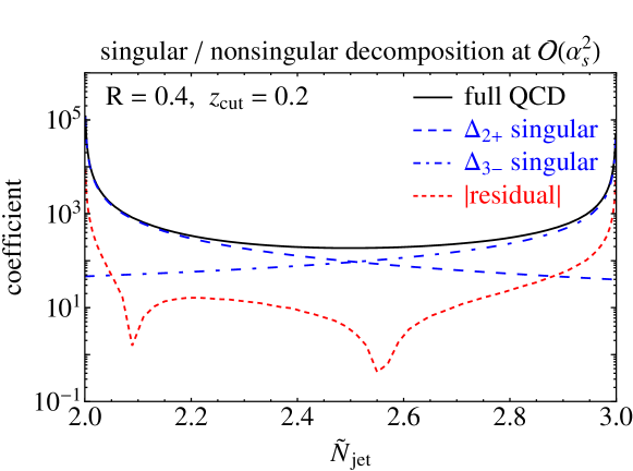
Figure 8: The $2<\widetilde{N}_{\rm jet}<3$ distribution in full QCD (black, solid), decomposed into singular contributions from $\Delta_{2+}$ and $\Delta_{3-}$ (blue, dashed/dot-dashed) and residual nonsingular contributions (red, dotted). The coefficient of $(\alpha_{s}/2\pi)^{2}$ is plotted for each contribution. Note that the sum of singular contributions is numerically dominant over the entire range.

Since we are mainly interested in describing the behavior in the vicinity of $\widetilde{N}_{\rm jet}=2$, though, for the rest of the paper we will simply adopt the nonsingular definition in Eq. (56), even in the vicinity of $\widetilde{N}_{\rm jet}=3$:

$$\frac{\text{d}\sigma_{\rm ns}}{\text{d}\widetilde{N}_{\rm jet}}(2<\widetilde{N}_{\rm jet}<3)=\frac{\text{d}\sigma_{\rm ns}}{\text{d}\Delta_{2+}}=\frac{\text{d}\sigma_{\rm full}}{\text{d}\widetilde{N}_{\rm jet}}-\frac{\text{d}\sigma_{\rm sing}}{\text{d}\Delta_{2+}}\,.$$ (57)

That said, this non-singular term turns out to be dominated by the singular $\Delta_{3-}$ piece. Writing the nonsingular term as

$$\frac{\text{d}\sigma_{\rm ns}}{\text{d}\Delta_{2+}}=\frac{\text{d}\sigma_{\rm sing}}{\text{d}\Delta_{3-}}+\frac{\text{d}\sigma_{\rm res}}{\text{d}\Delta_{2+}},$$ (58)

the residual term is quite small, even in the vicinity of $\widetilde{N}_{\rm jet}=2.5$. This is shown in Fig. 8, where the full QCD result between $2<\widetilde{N}_{\rm jet}<3$ is decomposed into the $\Delta_{2+}$ singular, $\Delta_{3-}$ singular, and residual terms for $R=0.4$ and $z_{\rm cut}=0.2$. The fact that the $\Delta_{2+}$ nonsingular term is nearly saturated by the $\Delta_{3-}$ singular term suggests that higher-order logarithmic terms can play an important role in determining the shape of the $\widetilde{N}_{\rm jet}$ distribution, even for large deviations from integer values of the observable.

4.3 Complete Results to Order $\alpha_{s}^{2}$

Summarizing the results from Secs. 4.1 and 4.2, the full $\mathcal{O}\!\left(\alpha_{s}^{2}\right)$ result for the near-integer $\Delta_{2\pm}$ distributions can be written as

$$\frac{\text{d}\sigma}{\text{d}\Delta_{2\pm}}=\underbrace{\left[\frac{\text{d}\sigma}{\text{d}\Delta_{2\pm}}\right]_{\rm ab}+\left[\frac{\text{d}\sigma}{\text{d}\Delta_{2\pm}}\right]_{\rm nab}+\left[\frac{\text{d}\sigma}{\text{d}\Delta_{2\pm}}\right]_{C_{F}T_{R}n_{f}}}_{\rm singular}\,+\;\frac{\text{d}\sigma_{\rm ns}}{\text{d}\Delta_{2\pm}}.$$ (59)

The first three terms in Eq. (59) are the singular contributions to the cross section. The Abelian terms are given in Eqs. (52) and (53), while the contributions of non-Abelian and $C_{F}T_{R}n_{f}$ color structures can be found in App. A. The last term in Eq. (59) is the nonsingular contribution that we extract numerically from Event2 as discussed above.

As discussed in Eq. (57), the entirety of the $\Delta_{3-}$ singular distribution in Eq. (54) has been absorbed into the $\Delta_{2+}$ nonsingular distribution. Thus, when we plot $\Delta_{3-}$ in Sec. 7, we are in effect plotting the prediction for $\Delta_{3-}=1-\Delta_{2+}$.

5 Towards a Factorization Theorem

In the previous section, we have seen that soft and collinear matrix elements govern the near-integer behavior of $\widetilde{N}_{\rm jet}$ in fixed-order QCD. In this section, we explore the all-orders behavior at and near $\widetilde{N}_{\rm jet}=2$, building a candidate factorization theorem to describe the logarithmically-enhanced contributions to the cross section.

Near $\widetilde{N}_{\rm jet}=2$, energetic collinear modes must be confined to two jet regions of diameter $R$, such that no two energetic particles are more than $R$ apart. This suggests that the collinear radiation may be described by jet functions. Additional radiation must be sufficiently soft so as not to create an additional jet, meaning there is a local veto of size $z_{\rm cut}$ outside of the primary jets. This suggests that additional radiation may be described by a soft function. However, while one might hope that a factorization theorem of the form

$$\sigma(\Delta_{2\pm})\sim\sigma_{0}\,H_{q\bar{q}}\Bigl{[}J_{q}(\Delta_{2\pm})\otimes J_{\bar{q}}(\Delta_{2\pm})\otimes S_{q\bar{q}}(\Delta_{2\pm})\Bigr{]}$$ (60)

would hold, it fails on several fronts. First, this standard factorization picture is challenged by both the non-additivity of the observable and soft-collinear non-factorization (discussed in Sec. 2.3 and examined in more detail below). Additionally, the logarithms of $\Delta_{2\pm}$ are non-global, and may not be summed with the above factorization into jet and soft functions. Furthermore, the cross section at $\widetilde{N}_{\rm jet}=2$ $(\Delta_{2\pm}=0)$ behaves similarly to a dijet cross section from a standard discrete jet algorithm, for which a convolution structure does not apply.

We will discuss these issues below, en route to a candidate “local” factorization theorem which applies in the small $R$ limit. This factorization theorem will take the form

$$\frac{\text{d}\sigma}{\text{d}\Delta_{2\pm}}=\sigma(\widetilde{N}_{\rm jet}=2)\Bigl{[}C_{q}(\Delta_{2\pm})\otimes C_{\bar{q}}(\Delta_{2\pm})\Bigr{]}\,,$$ (61)

where $\sigma(\widetilde{N}_{\rm jet}=2)$ is the cross section exactly at $\widetilde{N}_{\rm jet}=2$ (see Sec. 5.1) and $C_{q,\bar{q}}$ are “collinear functions” (see Sec. 5.3). This form satisfies a number of plausibility checks, but a formal proof of its validity is beyond the scope of the present paper.

5.1 The Cross Section at $\widetilde{N}_{\rm jet}=2$

We begin by considering the cross section at exactly $\widetilde{N}_{\rm jet}=2$. At $\mathcal{O}\!\left(\alpha_{s}\right)$, the constraints to obtain $\widetilde{N}_{\rm jet}=2$ are the same as for obtaining two jets from a discrete jet algorithm, namely that either two of the three partons must lie within a mutual radius of $R$ or one of the partons must be below $E_{{\rm cut}}$. At leading power, the phase space restrictions on the $q\overline{q}g$ final state are

$$\Theta(\theta_{qg}<R)+\Theta(\theta_{\bar{q}g}<R)+\Theta(\theta_{qg}>R)\Theta(\theta_{\bar{q}g}>R)\Theta(z_{g}<z_{\rm cut})\,.$$ (62)

At higher orders, the phase space restrictions differ from discrete jet algorithms (which also differ among themselves), and the $\widetilde{N}_{\rm jet}=2$ cross section has unique features. Consider an $\mathcal{O}\!\left(\alpha_{s}^{2}\right)$ configuration contributing to the near-integer behavior, as discussed in the Sec. 4.1. A concrete example is the $\Delta_{2+}$-$\mathcal{R}_{C}$ configuration in Table 1, which has a collinear $q\to qg$ splitting with another soft gluon (labeled $s$) emitted such that

$$\theta_{qg}<R\,,\quad\theta_{qs}>R\,,\quad\theta_{gs}<R\,.$$ (63)

This event will give a non-integer contribution to $\widetilde{N}_{\rm jet}$, and its contribution to the cross section is of the form

$$\sim\alpha_{s}^{2}\biggl{[}\frac{1}{\epsilon^{2}}\delta(\widetilde{N}_{\rm jet}-2)+\zeta\delta(\widetilde{N}_{\rm jet}-2)+\kappa_{0}\,\mathcal{L}_{0}(\Delta_{2+})+\kappa_{1}\,\mathcal{L}_{1}(\Delta_{2+})\biggr{]}\,.$$ (64)

The plus distribution terms were already calculated in Eq. (53). The $\delta(\Delta_{2+})$ terms were suppressed in our previous discussion (since we were focused on the non-integer behavior), but both the $1/\epsilon^{2}$ term and the $\zeta$ term follow directly from the calculations in Sec. 4.1.

The structure of Eq. (64) reflects the hybrid jet algorithm/event shape behavior of $\widetilde{N}_{\rm jet}$. The plus distribution terms have no support at $\widetilde{N}_{\rm jet}=2$, since the plus function prescription removes any divergence there. This feature is similar to other event shape variables with a singular limit, such as thrust, where there is zero cross section in the singular limit at higher orders. By contrast, the delta function terms behave more like a jet algorithm, as anticipated in Eq. (6), with a finite cross section at exactly $\widetilde{N}_{\rm jet}=2$. The IR pole from the real radiation at $\widetilde{N}_{\rm jet}=2$ will cancel divergences from virtual matrix elements, such that the $\widetilde{N}_{\rm jet}=2$ cross section is IR finite. The additional finite $\zeta$ term at $\widetilde{N}_{\rm jet}=2$ implies that the non-global structure in the near-integer part of the cross section is also contributing at $\widetilde{N}_{\rm jet}=2$.

5.2 Soft-Collinear Non-Factorization

The non-global nature of the near-integer behavior of $\widetilde{N}_{\rm jet}$ is suggestive of a non-standard picture of factorization. In fact, the $\widetilde{N}_{\rm jet}$ observable does not obey soft-collinear factorization, meaning separate soft and collinear functions cannot be easily (or usefully) defined. This was foreshadowed in Sec. 2.3 and can be illustrated with a simple example at $\mathcal{O}\!\left(\alpha_{s}^{2}\right)$.

Consider the same phase space configuration as Eq. (63), which has a single soft gluon and a pair of collinear (energetic) partons. The soft gluon is in the region of phase space where it is in the jet region of only one of the collinear partons, and the value of the observable is dependent on this fact. This implies that the observable receives contributions that intrinsically depend on the soft and collinear modes in a non-factorizable way; the measurement function cannot be separated into separate soft and collinear pieces that do not depend on each other (see Fig. 4). Therefore, soft-collinear factorization does not hold. We note that, unlike other cases where soft-collinear factorization is not straightforward (see, e.g., Walsh:2011fz ; Tackmann:2012bt ), here the leading non-integer behavior does not factorize.

Because the non-global structure of $\Delta_{2\pm}$ feeds into the $\widetilde{N}_{\rm jet}=2$ cross section through the $\zeta$ term in Eq. (64), the same non-factorization is also true of the integer value. Of course, for the exact $\widetilde{N}_{\rm jet}=2$ case, non-factorization of the soft and collinear modes happens only at $\mathcal{O}\!\left(\alpha_{s}^{2}\right)$. Therefore, one can write the $\widetilde{N}_{\rm jet}=2$ cross section as the sum of terms, one with global contributions that can consistently be resummed and one with non-factorizing contributions. Such a form is

$$\sigma(\widetilde{N}_{\rm jet}=2) =\sigma_{0}H_{q\bar{q}}(Q,\mu)J_{q}(Q,R,z_{\rm cut},\mu)J_{\bar{q}}(Q,R,z_{\rm cut},\mu)S_{q\bar{q}}(R,z_{\rm cut},\mu)$$

$$\quad+\sigma_{2}^{\rm non-fac}(Q,R,z_{\rm cut},\mu)\,.$$ (66)

The factorized part of the cross section is similar to dijet (or, generally, exclusive jet) cross sections. In $e^{+}e^{-}$ collisions, such cross sections are known to contain non-global logarithms that spoil a standard effective theory picture of the dynamics. These non-global logarithms span the jet and soft functions, affecting the RG evolution in nontrivial ways. Similar to the non-factorizing terms, the non-global contributions start at $\mathcal{O}\!\left(\alpha_{s}^{2}\right)$.

5.3 Introducing Collinear Functions

Let us now try to simultaneously describe the near-integer and exact-integer behavior of $\widetilde{N}_{\rm jet}$. We have established that the logarithms of $\Delta_{2\pm}$ are purely non-global, and there is no standard soft-collinear factorization. As mentioned in Sec. 2.3, however, the contributions from each jet region are independent, meaning they can be separated:

$$\frac{\text{d}\sigma}{\text{d}\Delta_{2\pm}}\sim\sigma_{0}\,C_{q}(\Delta_{2\pm})\otimes C_{\bar{q}}(\Delta_{2\pm})\,,$$ (67)

where $\sigma_{0}$ is an overall prefactor and $\otimes$ refers to the standard convolution in Eq. (94). Here, we have introduced “collinear functions” $C_{q}$ and $C_{\bar{q}}$ for the two jet regions, which give the contribution to $\Delta_{2\pm}$ for each jet region separately.

The collinear functions contain only the singular terms and have the general form

$$C_{q,\bar{q}}(\Delta_{2\pm}) =\delta(\Delta_{2\pm})+\sum_{n=2}^{\infty}\Bigl{(}\frac{\alpha_{s}}{\pi}\Bigr{)}^{n}\sum_{k=-1}^{n-1}\Bigl{[}\kappa_{k,+}^{(n)}\,\mathcal{L}_{k}(\Delta_{2+})+\kappa_{k,-}^{(n)}\,\mathcal{L}_{k}(\Delta_{2-})\Bigr{]}\,,$$ (68)

where $\kappa_{k,\pm}^{(n)}$ are coefficients which in general depend on $z_{\rm cut}$ (except for the leading coefficient $\kappa_{n-1,\pm}^{(n)}$). Recall that $\mathcal{L}_{-1}(x)=\delta(x)$, and these delta functions are needed to describe the $\widetilde{N}_{\rm jet}=2$ cross section. Since $\Delta_{2\pm}$ describe different regimes of the same observable ($\widetilde{N}_{\rm jet}$ just above/below 2), each term in the expansion has support for one term or the other.

The convolution between the collinear functions in Eq. (67) mixes the distributions for $\Delta_{2+}$ and $\Delta_{2-}$. Therefore, we require not only the usual convolutions between distributions of either $\Delta_{2+}$ or $\Delta_{2-}$ (which we refer to as convolutions of one-sided distributions, e.g. $\mathcal{L}_{0}(\Delta_{2+})\otimes\mathcal{L}_{0}(\Delta_{2+})$), but also convolutions between distributions of $\Delta_{2+}$ and $\Delta_{2-}$ (which we refer to as convolutions of two-sided distributions, e.g. $\mathcal{L}_{0}(\Delta_{2+})\otimes\mathcal{L}_{0}(\Delta_{2-})$). Details about the definitions of one- and two-sided distributions and convolutions between them are presented in App. B.

We can now reinterpret the calculation in Sec. 4.1 directly as a calculation of $C_{q}$ and $C_{\bar{q}}$ to $\mathcal{O}\!\left(\alpha_{s}^{2}\right)$ (see App. C). The convolution between $C_{q}$ and $C_{\bar{q}}$ in Eq. (67) then gives part of the higher-order $\mathcal{O}\!\left(\alpha_{s}^{4}\right)$ cross section. In addition, we can estimate the $\mathcal{O}\!\left(\alpha_{s}^{4}\right)$ structure of an individual collinear function by performing naïve (Abelian) exponentiation to capture some of the multiple emission terms. That is, we assume that each of the collinear functions in Eq. (68) has the form

$$\begin{split}C_{q,\bar{q}}(\Delta_{2\pm})&=\delta(\Delta_{2\pm})+\Bigl{(}\frac{\alpha_{s}(\mu)}{\pi}\Bigr{)}^{2}\Bigl{[}\mathcal{K}_{+}(\Delta_{2+})+\mathcal{K}_{-}(\Delta_{2-})\Bigl{]}\\ &\quad+\frac{1}{2}\Bigl{(}\frac{\alpha_{s}(\mu)}{\pi}\Bigr{)}^{4}\Bigl{[}\mathcal{K}_{+}(\Delta_{2+})+\mathcal{K}_{-}(\Delta_{2-})\Bigl{]}\otimes\Bigl{[}\mathcal{K}_{+}(\Delta_{2+})+\mathcal{K}_{-}(\Delta_{2-})\Bigl{]}\,,\end{split}$$ (69)

where

$$\mathcal{K}_{+}(\Delta_{2+}) =\kappa_{0,+}^{(2)}\mathcal{L}_{0}(\Delta_{2+})+\kappa_{1,+}^{(2)}\mathcal{L}_{1}(\Delta_{2+})\,,$$ (70)

$$\mathcal{K}_{-}(\Delta_{2-}) =\kappa_{0,-}^{(2)}\mathcal{L}_{0}(\Delta_{2-})+\kappa_{1,-}^{(2)}\mathcal{L}_{1}(\Delta_{2-})\,.$$ (71)

The convolution terms at $\mathcal{O}(\alpha_{s}^{4})$ are those coming from naïve Abelian exponentiation in one jet region. Note that this does not fully capture the correct higher-order terms (for example, we do not get any term at $\mathcal{O}(\alpha_{s}^{3})$ from this exponentiation), but we will see in Sec. 7 that it is enough to reproduce some of the higher-order effects observed in parton shower Monte Carlo generators. In defining Eq. (69), we have used the fact that one can absorb corrections to the $\widetilde{N}_{\rm jet}=2$ cross section into the $\sigma_{0}$ prefactor (see further discussion below).

5.4 A “Local” Factorization Theorem

Via Eq. (67), we can capture the impact on $\widetilde{N}_{\rm jet}$ of soft and collinear emissions within the two jet regions. But soft emissions away from the jet regions can still give logarithmically-enhanced contributions to the cross section, even if they do not change the value of $\widetilde{N}_{\rm jet}$. For example, a soft gluon well-separated from the jets with energy fraction less than $z_{\rm cut}$ will not change $\widetilde{N}_{\rm jet}$, but it will contribute to the cross section. For $e^{+}e^{-}\to q\bar{q}g$, this wide-angle soft radiation is part of the $\widetilde{N}_{\rm jet}=2$ phase space. Going to higher orders, there is a contribution to both the exact-integer and near-integer cross sections from wide-angle soft radiation, and up to power corrections for small $R$, both contributions are identical.

This logic implies that the $\widetilde{N}_{\rm jet}=2$ cross section should multiply the near-integer contributions, leading to the candidate factorization theorem from Eq. (61), repeated for convenience:

$$\frac{\text{d}\sigma}{\text{d}\Delta_{2\pm}}=\sigma(\widetilde{N}_{\rm jet}=2)\Bigl{[}C_{q}(\Delta_{2\pm})\otimes C_{\bar{q}}(\Delta_{2\pm})\Bigr{]}\,.$$ (72)

This is the same structure as Eq. (67), but we have identified $\sigma_{0}$ with $\sigma(\widetilde{N}_{\rm jet}=2)$. As discussed in Eq. (5.2), $\sigma(\widetilde{N}_{\rm jet}=2)$ itself has its own quasi-factorization theorem. If this candidate factorization theorem is indeed true, then the definition of $C_{q,\bar{q}}(\Delta_{2\pm})$ in Eq. (69) should be revised such that the coefficient of the $\delta(\Delta_{2\pm})$ piece is always 1 (i.e. the sum over $k$ should start at $0$ instead of $-1$).

We stress here that Eq. (61) is only a candidate factorization theorem, and we have not proven that such a form exists. In particular, we do not have an operator definition of the collinear functions $C_{q,\bar{q}}$, and without such a definition, the extraction of $C_{q,\bar{q}}$ is ambiguous from fixed-order calculations alone. The reason is that the structure of $C_{q}(\Delta_{2\pm})\otimes C_{\bar{q}}(\Delta_{2\pm})$ is single-logarithmic order-by-order, without any definite relation between coefficients, so higher-order terms can absorb corrections from lower-order ones. For example, the leading nontrivial terms in $\sigma(\widetilde{N}_{\rm jet}=2)$ (the $\mathcal{O}\!\left(\alpha_{s}\right)$ term) and $C_{q}(\Delta_{2\pm})\otimes C_{\bar{q}}(\Delta_{2\pm})$ (the $\mathcal{O}\!\left(\alpha_{s}^{2}\mathcal{L}_{1}\right)$ terms) will contribute to $\kappa_{1,\pm}^{(3)}$ (the $\mathcal{O}\!\left(\alpha_{s}^{3}\right)\mathcal{L}_{1}(\Delta_{2\pm})$ terms), but cannot unambiguously determine that coefficient.

Despite these limitations, our candidate factorization theorem does describe important effects (like convolutions between the two jet regions) that go beyond a simple perturbative, log series expansion, which is why we will use Eq. (61) in our comparison studies in Sec. 7. One thing we can say unambiguously is that if the factorization theorem in Eq. (61) is valid, then the collinear functions must be RG independent. The reason is that the prefactor $\sigma(\widetilde{N}_{\rm jet}=2)$ is itself a cross section, so it must be RG independent, and therefore $C_{q}\otimes C_{\bar{q}}$ must be RG independent. Similarly, the modes that contribute to $C_{q}$ and $C_{\bar{q}}$ are completely disjoint, so there is no possibility that RG-scale-dependence could cancel between $C_{q}$ and $C_{\bar{q}}$. This does not rule out, however, a further factorization of the collinear functions.

5.5 Complete Results

Let us summarize our final prediction for the $\Delta_{2\pm}$ distributions using the candidate factorization theorem in Eq. (61). Beyond the calculation summarized in Sec. 4.3, we can include two higher-order effects.

First, as described in Sec. 5.3, the collinear function approach allows us to capture $\mathcal{O}\!\left(\alpha_{s}^{4}\right)$ terms coming from convolutions. There are two types of convolutions: convolutions between $C_{q}$ and $C_{\bar{q}}$ given by the factorization theorem, and convolutions within an individual collinear function coming from naïve Abelian exponentiation. Though the naïve exponentiation can in principle give results to all orders in $\alpha_{s}$, we will truncate the convolutions to order $\mathcal{O}\!\left(\alpha_{s}^{4}\right)$, especially since there are known $\mathcal{O}\!\left(\alpha_{s}^{3}\right)$ terms missed by this approach.

Second, we can include running coupling effects by evaluating $\alpha_{s}(\mu)$ at an energy scale $\mu=Q\sqrt{\Delta_{2\pm}}$. To see why this is the correct scale, note that in Sec. 4.1, the fixed-order expansion in dim reg had a prefactor of

$$\biggl{(}\frac{\mu^{2}}{E_{J}^{2}\Delta_{2\pm}}\biggr{)}^{2\epsilon}\,,$$ (73)

where $E_{J}\simeq Q/2$ is the jet energy. This implies that at higher orders, the fixed-order calculation generates terms like $\ln(\mu^{2}/E_{J}^{2}\Delta_{2\pm})$ where $\mu$ is the renormalization scale, suggesting that $Q\sqrt{\Delta_{2\pm}}$ is a relevant running coupling energy scale.

As in Sec. 4.3, the nonsingular contributions to the cross section enter at fixed $\mathcal{O}\!\left(\alpha_{s}^{2}\right)$ and can be simply included additively. Like in Sec. 4.3, we absorb the entirety of the $\Delta_{3-}$ singular distribution into the $\Delta_{2+}$ nonsingular distribution. To try to capture some higher-order effects in $\Delta_{3-}$, though, we make use of the nonsingular decomposition in Eq. (58), repeated for convenience:

$$\frac{\text{d}\sigma_{\rm ns}}{\text{d}\Delta_{2+}}=\frac{\text{d}\sigma_{\rm sing}}{\text{d}\Delta_{3-}}+\frac{\text{d}\sigma_{\rm res}}{\text{d}\Delta_{2+}}.$$ (74)

We evaluate the singular $\Delta_{3-}$ piece at the scale $\mu=Q\sqrt{\Delta_{3-}}$ and the small $\Delta_{2+}$ residual term at a fixed scale $\mu=Q$. While this approach misses out on genuine $\mathcal{O}\!\left(\alpha_{s}^{3}\right)$ fixed-order corrections from 3-jet events, they have an endpoint at $\Delta_{3-}=(z_{\rm cut}/2)^{2}$ analogous to Eq. (30), so we will simply not make a prediction for $\Delta_{3-}<(z_{\rm cut}/2)^{2}$.

Finally, while the singular terms for $\Delta_{2\pm}$ come with an overall prefactor of $\sigma(\widetilde{N}_{\rm jet}=2)$, the nonsingular terms do not. However, since the nonsingular terms start at $\mathcal{O}\!\left(\alpha_{s}^{2}\right)$, we can multiply them by $\sigma(\widetilde{N}_{\rm jet}=2)/\sigma_{0}$, which introduces corrections beyond the order to which we are working. This allows us to factor out a global $\sigma(\widetilde{N}_{\rm jet}=2)$ from our final predictions.

Putting these pieces together, our final analytic prediction for the $\Delta_{2\pm}$ distribution is:

$$\frac{\text{d}\sigma}{\text{d}\Delta_{2\pm}} =\sigma(\widetilde{N}_{\rm jet}=2)\,\Bigl{\{}C_{q}(\Delta_{2\pm})\otimes C_{\bar{q}}(\Delta_{2\pm})+\frac{1}{\sigma_{0}}\frac{\text{d}\sigma_{\rm ns}}{\text{d}\Delta_{2\pm}}\Bigr{\}}$$ (75)

$$=\sigma(\widetilde{N}_{\rm jet}=2)\biggl{\{}\delta(\Delta_{2\pm})+2\Bigl{(}\frac{\alpha_{s}(Q\sqrt{\Delta_{2\pm}})}{\pi}\Bigr{)}^{2}\Bigl{[}\mathcal{K}_{+}(\Delta_{2+})+\mathcal{K}_{-}(\Delta_{2-})\Bigl{]}$$

$$\quad+2\Bigl{(}\frac{\alpha_{s}(Q\sqrt{\Delta_{2\pm}})}{\pi}\Bigr{)}^{4}\Bigl{[}\mathcal{K}_{+}(\Delta_{2+})+\mathcal{K}_{-}(\Delta_{2-})\Bigl{]}\otimes\Bigl{[}\mathcal{K}_{+}(\Delta_{2+})+\mathcal{K}_{-}(\Delta_{2-})\Bigl{]}$$

$$\quad+\frac{1}{\sigma_{0}}\frac{\text{d}\sigma_{\rm ns}}{\text{d}\Delta_{2\pm}}\biggl{\}}\,.$$

In Fig. 9, we compare the pure fixed $\mathcal{O}\!\left(\alpha_{s}^{2}\right)$ distributions for $\Delta_{2\pm}$ and $\Delta_{3-}$ from Eq. (59) with the final prediction from Eq. (75). At small values of $\Delta_{n\pm}$, the dominant differences come from the higher-order logarithms included in our final prediction, while at larger values of $\Delta_{n\pm}$ the running effects from our $\Delta_{n\pm}$-dependent scale choice give most of the difference from the fixed-order prediction. Since we do not have a candidate factorization theorem for the $\widetilde{N}_{\rm jet}=3$ region of phase space, the $\Delta_{3-}$ distribution is really just Eq. (75) evaluated at $\Delta_{3-}=1-\Delta_{2+}$.

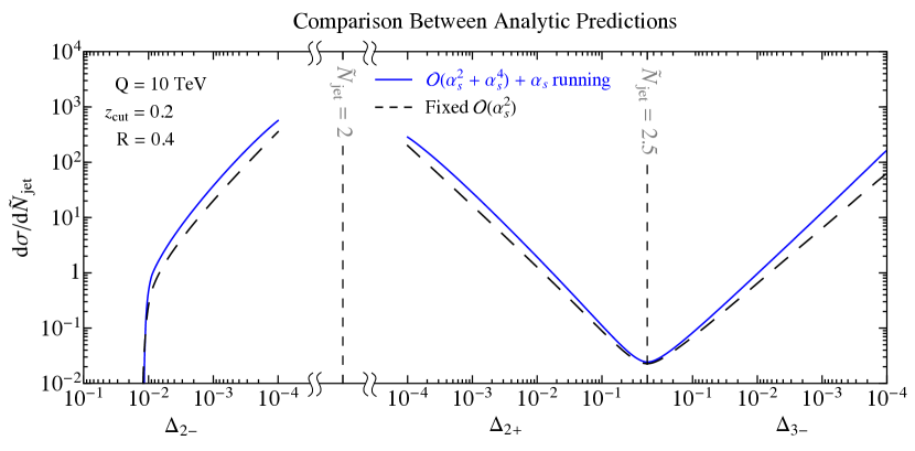
Figure 9: A comparison between analytic predictions for the $\widetilde{N}_{\rm jet}$ distribution. Shown in dashed black are the fixed $\mathcal{O}\!\left(\alpha_{s}^{2}\right)$ calculations from Eq. (59). Shown in solid blue are our final predictions from Eq. (75), which include an estimate of higher-order $\mathcal{O}\!\left(\alpha_{s}^{4}\right)$ terms as well as $\Delta_{2\pm}$-dependent running of $\alpha_{s}$. Note that the $\Delta_{2-}$ and $\Delta_{3-}$ axes run backwards.

6 Looking Towards the LHC

Given the interesting features of $\widetilde{N}_{\rm jet}$ and the wide-ranging and robust measurements of jet substructure at the LHC Abdesselam:2010pt ; Altheimer:2012mn ; Altheimer:2013yza , a natural consideration is the $\widetilde{N}_{\rm jet}$ distribution in hadronic collisions. In this case, it is more convenient to use the original definition of $\widetilde{N}_{\rm jet}$ from Eq. (1) based on transverse momenta and rapidity-azimuth distances (instead of energies and angles):

$$\widetilde{N}_{\rm jet}(p_{T{\rm cut}},R)=\sum_{i\in\text{event}}\frac{p_{Ti}}{p_{Ti,R}}\,\Theta(p_{Ti,R}-p_{T{\rm cut}}),$$ (76)

where $p_{Ti,R}=\sum_{j}p_{Tj}\,\Theta(R-R_{ij})$ and $R_{ij}=\sqrt{\Delta y_{ij}^{2}+\Delta\phi_{ij}^{2}}$.

At first glance, the calculation of $\widetilde{N}_{\rm jet}$ at the LHC would seem to be much more difficult than at an $e^{+}e^{-}$ collider. After all, $\widetilde{N}_{\rm jet}$ depends sensitively on soft radiation, and soft QCD is notoriously complicated at a hadron collider. However, $\widetilde{N}_{\rm jet}$ only depends on soft radiation in a region of size $\lesssim 2R$ around energetic partons. To the extent that we can exploit color coherence at small $R$, we can make predictions for $\widetilde{N}_{\rm jet}$ by simply knowing the collinear functions for quark- and gluon-initiated jets, $C_{q}$ and $C_{g}$. In particular, the $1\to 3$ splitting function formalism that we used in Sec. 4.1 to calculate the collinear function for quarks in $e^{+}e^{-}$ may also be used to calculate the quark and gluon collinear functions for LHC processes.

Conveniently, when switching between the $e^{+}e^{-}$ and hadronic definitions of $\widetilde{N}_{\rm jet}$, the collinear functions $C_{q,g}$ only differ by terms of $\mathcal{O}(R)$. For small jet radii, one can therefore neglect those corrections and use the $e^{+}e^{-}$ collinear functions calculated in this paper also for the hadronic case, though one has to be careful to match the $z_{\rm cut}$ value to the outgoing parton momentum. To see why this is the case, notice that

$$z_{i}=\frac{E_{i}}{E_{J}}\simeq\frac{p_{Ti}}{p_{TJ}}[1+\mathcal{O}(R)],\qquad z_{\rm cut}=\frac{E_{{\rm cut}}}{E_{J}}\simeq\frac{p_{T{\rm cut}}}{p_{TJ}}[1+\mathcal{O}(R)],$$ (77)

where $p_{TJ}$ is the scalar sum of transverse momenta in a jet region. Thus, the energy integrals in $C_{q,g}$ would differ at most by $\mathcal{O}(R)$ terms. The angular phase space regions in Eq. (36) would be written as constraints on $R_{ij}$ instead of $\theta_{ij}$, but notice that

$$R_{ij}=\theta_{ij}(\cosh y_{i}\cosh y_{j})^{1/2}\simeq\theta_{ij}\cosh y_{J}[1+\mathcal{O}(R)],$$ (78)

where $y_{J}$ is some characteristic rapidity associated with the jet region, for example the rapidity of the summed jet region momenta. At leading power, the logarithmic scaling of the angular integrals can be used to remove any dependence on $\cosh y_{J}$, so that the differences in the angular integrals are again at most an $\mathcal{O}(R)$ effect.

In order to extend the candidate dijet factorization formula in Eq. (61) to dijet events from hadronic collisions, we have to sum over all relevant partonic channels:

$$\frac{\text{d}\sigma}{\text{d}\Delta_{2\pm}}=\sum_{k,\ell}\sigma_{h_{1}h_{2}\to k\ell}(\widetilde{N}_{\rm jet}=2)\,C_{k}(\Delta_{2\pm})\otimes C_{\ell}(\Delta_{2\pm})\,,$$ (79)

where $k,\ell=q$, $\bar{q}$, or $g$, and $h_{1,2}$ represents the colliding hadrons. In general, $\sigma_{h_{1}h_{2}\to k\ell}$, $C_{k}$, and $C_{\ell}$ depend on the outgoing parton kinematics, though we have suppressed that dependence in Eq. (79) for readability. Note that the incoming beams only create additional high-$p_{T}$ jets through hard, perturbative emissions. We can write the total rate $\sigma_{h_{1}h_{2}\to k\ell}(\widetilde{N}_{\rm jet}=2)$ schematically as

$$\sigma_{h_{1}h_{2}\to k\ell}(\widetilde{N}_{\rm jet}=2)=\sum_{a,b}\int_{0}^{1}\text{d}x_{a}\,\text{d}x_{b}\,f_{a/h_{1}}(x_{a})f_{b/h_{2}}(x_{b})\,\sigma_{ab\to k\ell}(\widetilde{N}_{\rm jet}=2),$$ (80)

where $f_{a/h_{1}}$ and $f_{b/h_{2}}$ are parton distribution functions for partons $a$ and $b$ carrying momentum fractions $x_{a,b}$ of the initial hadrons $h_{1,2}$, and $\sigma_{ab\to k\ell}(\widetilde{N}_{\rm jet}=2)$ is the total rate at $\widetilde{N}_{\rm jet}=2$ for the partonic channel $ab\to k\ell$. As in the $e^{+}e^{-}$ case, this cross section can have large logarithms of $R$ and $p_{T{\rm cut}}$ that require resummation to obtain reliable predictions.

Compared to the $e^{+}e^{-}$ case, the main new ingredient is the collinear function $C_{g}(\Delta_{2\pm})$ for a gluon-initiated jet. For completeness, we have calculated the gluon collinear function using the same approach as Sec. 4.1, and we present both $C_{q}$ and $C_{g}$ in App. C. The structure in Eq. (79) can be easily extended to handle the $\Delta_{n\pm}$ cross section for $n$-jet processes by using $n$ collinear functions multiplied by the $\widetilde{N}_{\rm jet}=n$ cross section, appropriately summed over the various partonic channels.

At a hadron collider, there is also a new potential source of non-global logarithms from initial state partons. In general, non-global logarithms of $\Delta_{n\pm}$ only appear in the collinear functions $C_{q,g}$ for each final state jet, and are associated with correlated emissions from final state partons. For events with well-separated jets, the collinear functions are universal and independent of other jets in the event. However, there are also non-global logarithms of $z_{\rm cut}$ and $R$ which appear both in the collinear functions and in the exact integer $\widetilde{N}_{\rm jet}$ cross section (e.g. $\sigma_{h_{1}h_{2}\to k\ell}(\widetilde{N}_{\rm jet}=2)$, see Eq. (5.2)). For the exact integer cross section at a hadron collider, one also has to include correlated emissions from initial state partons, which may introduce super-leading logarithms Forshaw:2006fk ; Forshaw:2008cq ; Keates:2009dn at sufficiently high $\alpha_{s}$ order. Ideally, one would want to understand the resummation of non-global effects in the collinear functions and the exact integer cross section to achieve accurate predictions.

Because a detailed study for the LHC is beyond the scope of this paper, we will not present any results for hadronic collisions. An important effect to account for in future LHC predictions and comparisons with measurements is hadronization, which we have not considered here. Additionally, for hadronic collisions, effects from the underlying event and initial state radiation are not present in the $e^{+}e^{-}$ case. To lowest order in $R$, we expect those effects to be captured by color coherence, and one could imagine using the techniques of Ref. Stewart:2014nna to understand the $R$ dependence. A similar concern is pileup contamination, though the closed-form nature of $\widetilde{N}_{\rm jet}$ makes it well-suited to analytic studies using area subtraction Cacciari:2007fd ; Cacciari:2008gn ; Soyez:2012hv . One could further mitigate the impact of pileup by using a version of $\widetilde{N}_{\rm jet}$ that includes jet trimming Krohn:2009th in closed form Bertolini:2013iqa , and we expect the collinear function for the trimmed $\widetilde{N}_{\rm jet}$ version could be calculated using the same techniques used here.

7 Monte Carlo Comparisons

We now compare our analytic prediction in Eq. (75) with parton shower Monte Carlo generators. As discussed in Sec. 5.4, the rate $\sigma(\widetilde{N}_{\rm jet}=2)$ only enters as an overall normalization factor, and it in principle requires resummation of logarithms of $R$ and $z_{\rm cut}$ to obtain a reliable prediction. Since we are mainly interested in describing only the near-integer (and not the exact-integer) behavior, we will divide out by an overall normalization factor and perform only a shape comparison. In all of the plots below, we normalize the cross section to the region $\Delta_{2+}\in(10^{-4},10^{-2})$.

To make an apples-to-apples comparison of our analytic results to Pythia 8 and Herwig++, we turn off hadronization in the Monte Carlo generators. In principle, the collinear functions $C_{q}$ and $C_{\bar{q}}$ should get hadronization corrections, but the non-factorizing nature of $\widetilde{N}_{\rm jet}$ means that we cannot adopt a standard shape function analysis Korchemsky:1999kt ; Korchemsky:2000kp . We run at a sufficiently high energy to allow for a comparison over a wide logarithmic range in $\Delta_{2\pm}$. The large collision energy we choose, $Q=10$ TeV, also mitigates the effect of low energy cutoffs ($\simeq 1$ GeV) on the parton shower.

Because the singular terms in our calculation are numerically dominant for small $\Delta_{2\pm}$, higher-order logarithms may be important in determining the shape of the distribution in this regime. Some of the $\mathcal{O}\!\left(\alpha_{s}^{4}\right)$ effects are captured by the convolution structure in Eq. (75), but they are not fully reliable. Therefore, we include an uncertainty in our predictions derived from the addition of $\mathcal{O}\!\left(\alpha_{s}^{3}\mathcal{L}_{2}(\Delta_{2\pm})\right)$ and $\mathcal{O}\!\left(\alpha_{s}^{4}\mathcal{L}_{3}(\Delta_{2\pm})\right)$ terms with unknown coefficients that we vary. These terms represent the leading logarithms at each order, and are an estimate of missing higher-order terms. The form we use to determine the uncertainty is

$$\frac{\text{d}\sigma}{\text{d}\Delta_{2\pm}}\supset\Bigl{(}\frac{\alpha_{s}}{\pi}\Bigr{)}^{3}\kappa^{(3)}_{2,\pm}\mathcal{L}_{2}(\Delta_{2\pm})+\Bigl{(}\frac{\alpha_{s}}{\pi}\Bigr{)}^{4}\kappa^{(4)}_{3,\pm}\mathcal{L}_{3}(\Delta_{2\pm}),$$ (81)

and we vary independently the coefficients in the ranges $\kappa^{(3)}_{2,\pm}\in(-5,5)$ and $\kappa^{(4)}_{3,\pm}\in(-15,15)$. These coefficients are of similar size as the leading coefficients $\kappa^{(2)}_{1,\pm}$ in our calculation, and the $\mathcal{O}\!\left(\alpha_{s}^{4}\right)$ term generated by the naïve exponentiation in Eq. (75) has $\kappa^{(4)}_{3,\pm}\sim\mathcal{O}\!\left(10\right)$. The uncertainty band is given by the envelope of these variations, including effects both on the cross section normalization (where we just add Eq. (81)) and on the cross section shape (where we add Eq. (81) and readjust the normalization in the $\Delta_{2+}\in(10^{-4},10^{-2})$ window).

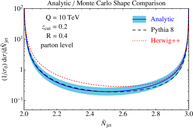
Figure 10: A shape comparison between our analytic predictions for the $2<\widetilde{N}_{\rm jet}<3$ distribution with the Monte Carlo generators Pythia 8 and Herwig++. Our calculation is summarized in Eq. (75) with uncertainties given in Eq. (81). To make an apples-to-apples comparison, we include showering but not hadronization in the Monte Carlo samples. All cross sections are normalized to have the same value in the $\Delta_{2+}\in(10^{-4},10^{-2})$ window.

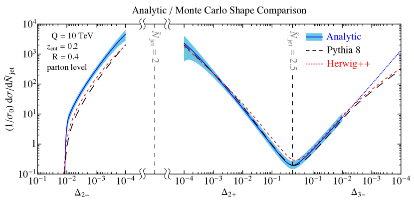
Figure 11: Same distributions as Fig. 10, but in triptych form to highlight the near integer behavior. Because we normalize only to the $\Delta_{2+}\in(10^{-4},10^{-2})$ window, the normalization differences in the $\Delta_{2-}$ region are accentuated; the shape agreement is much better. For the $\Delta_{3-}$ distribution, we extend our central prediction (with a dotted blue line) to $\Delta_{3-}<(z_{\rm cut}/2)^{2}$, where genuine 3-jet events, whose contribution we have not calculated, contribute to the observable. Note that the $\Delta_{2-}$ and $\Delta_{3-}$ axes run backwards.

In Fig. 10, we show the shape comparison between our result and Pythia 8/Herwig++ over the range $2<\widetilde{N}_{\rm jet}<3$. The singular cross section for $\Delta_{3-}$ is included as part of the nonsingular correction to the $\Delta_{2+}$ distribution (see Eq. (74)). Overall, we find good agreement with the Monte Carlo generators within uncertainties. It is amusing that there is such close agreement with Pythia 8 in the $\widetilde{N}_{\rm jet}\to 2$ region and with Herwig++ in the $\widetilde{N}_{\rm jet}\to 3$ region, with the analytic result effectively interpolating between the two. Given that the $\Delta_{2+}$ and $\Delta_{3-}$ parts of the distribution are dominated by different phase space configurations (see Table 1), it is possible that we are seeing the impact of different shower ordering variables in Pythia 8 ($p_{\perp}$-ordered) versus Herwig++ (angular-ordered). Of course, the theoretical uncertainties in our calculation are too large to make a definitive statement.

In Fig. 11, we compare distributions of $\Delta_{2\pm}$ over the range $(10^{-4},1)$, using the triptych format to also see the $\Delta_{3-}$ region. Again, our analytic prediction reproduces the shape of the Pythia 8 and Herwig++ distributions remarkably well over the whole range. The Monte Carlo distributions, which include higher-order logarithms of $\Delta_{2\pm}$ through multiple emissions, generally lie within the uncertainty band of our prediction for $\widetilde{N}_{\rm jet}>2$. This indicates that we have made a reasonable estimate of the higher-order corrections not included in our calculation. Because we normalize to the window $\Delta_{2+}\in(10^{-4},10^{-2})$, it is not surprising that there is a normalization discrepancy in $\Delta_{2-}$, though one can see that the shape agreement for $\widetilde{N}_{\rm jet}<2$ is excellent. We suspect that the normalization issues for $\widetilde{N}_{\rm jet}<2$ may be due to the treatment of correlated soft radiation (and angular ordering) in the Monte Carlo generators, since the $\Delta_{2-}$ distribution is dominated by double-soft emissions with a $C_{F}C_{A}$ color structure. The overall shape agreement between Pythia 8 and Herwig++ is quite surprising, given that they exhibit a factor of 3 difference (not shown) in their predicted value of $\sigma(\widetilde{N}_{\rm jet}=2)$, suggesting that the shape of the non-integer distributions is more robust than the cross section at integer values.

8 Conclusions

In this paper, we studied the analytic properties of $\widetilde{N}_{\rm jet}$, a jets-without-jets event shape that can return a fractional value of jet multiplicity. Focusing on $e^{+}e^{-}\to\text{jets}$, we calculated the distribution of $\widetilde{N}_{\rm jet}$ in the vicinity of a dijet configuration at $\mathcal{O}\!\left(\alpha_{s}^{2}\right)$. A fractional number of jets requires at least three collimated partons, such that for $e^{+}e^{-}\to\text{jets}$, the first non-trivial contribution requires at least two emissions. The singular parts of this emission structure can be captured using $1\to 3$ splitting functions, and we validated this approach (and included nonsingular contributions) using the fixed-order code Event2. To partially capture higher-order effects out to $\mathcal{O}\!\left(\alpha_{s}^{4}\right)$, we included convolutions from different phase space regions and running coupling effects. We found very good agreement between our calculation and Monte Carlo distributions from both Pythia 8 and Herwig++.

Fractional jet multiplicity exhibits unique analytic features that are not shared by other jet observables. At $\mathcal{O}\!\left(\alpha_{s}^{2}\right)$, we showed how rapidity-like divergences, related to the energy sharing between emissions, appear when one or two partons become soft, and we explained how to regulate them. Beyond the fixed-order result, we proposed a candidate local factorization theorem and used it to predict a hybrid jet algorithm/event shape behavior for the $\widetilde{N}_{\rm jet}$ distribution in the vicinity of an integer. At exact-integer values, $\widetilde{N}_{\rm jet}$ behaves much like a standard jet algorithm, yielding spikes in the $\widetilde{N}_{\rm jet}$ cross section. The near-integer behavior of $\widetilde{N}_{\rm jet}$ is more characteristic of event shapes, where towers of higher-order logarithms give rise to (single-logarithmic) suppression of the singular phase space, yielding shoulders in the $\widetilde{N}_{\rm jet}$ cross section. Finally, as opposed to typical event shapes, collinear emissions do not generate logarithms of $\widetilde{N}_{\rm jet}$, so the shape of the near-integer distribution is entirely determined by soft logarithms. These soft logarithms are purely non-global, as near-integer values force soft partons to lie in a restricted angular region of phase space and correlate different emissions (even if generated from an Abelian matrix element).

Beyond our present understanding of $\widetilde{N}_{\rm jet}$, there are three key directions to pursue. The first is to extend our calculations to $\mathcal{O}\!\left(\alpha_{s}^{3}\right)$. Though the differential cross section shapes were largely within our uncertainty estimates, the normalization differences seen between our analytic calculations and Monte Carlo generators suggest that higher-order terms might be relevant. While we were able to estimate some $\mathcal{O}\!\left(\alpha_{s}^{4}\right)$ effects through convolutions, there are genuine $\mathcal{O}\!\left(\alpha_{s}^{3}\right)$ effects that may get a phase space enhancement in the merged jet region (relative to the $\mathcal{O}\!\left(\alpha_{s}^{2}\right)$ phase space) to partially overcome the $\alpha_{s}$ suppression. The second is to attempt an understanding of logarithmic resummation. Because of the non-global nature of the observable, standard renormalization group methods will not work, but there may be a way to exploit the rapidity-like divergences seen in Sec. 3 or the techniques introduced in Refs. Larkoski:2015zka ; Caron-Huot:2015bja . The third is to perform a detailed study for hadron colliders like the LHC, as discussed in Sec. 6, including the important effect of hadronization. Fractional jets offer a more nuanced understanding of jet formation than is possible with standard jet algorithms, and a measurement of $\widetilde{N}_{\rm jet}$ seems feasible given the increasingly sophisticated approach to jet physics at the LHC.

Appendix A Results for Non-Abelian Contributions

Following the Abelian results in Sec. 4.1, here we show the singular $C_{F}C_{A}$ and $C_{F}T_{R}n_{f}$ contributions to the $\Delta_{2\pm}$ and $\Delta_{3-}$ cross sections. The $C_{F}C_{A}$ terms are

$$\left[\frac{\text{d}\sigma}{\text{d}\Delta_{2-}}\right]_{\rm nab} =\left(\frac{\alpha_{s}}{\pi}\right)^{2}C_{F}C_{A}\biggl{\{}-\frac{14}{5}\mathcal{I}_{\Omega}\mathcal{L}_{1}(\Delta_{2-})$$ (82)

$$\qquad\qquad\qquad\qquad+\biggl{[}\frac{28}{5}\mathcal{I}_{\Omega}\ln z_{\rm cut}+\mathcal{I}_{\Omega}^{(a)}\biggr{]}\mathcal{L}_{0}(\Delta_{2-})\biggr{\}}\Theta(\Delta_{2-}<z_{\rm cut}^{2}/4)\,,$$

$$\left[\frac{\text{d}\sigma}{\text{d}\Delta_{2+}}\right]_{\rm nab} =\left(\frac{\alpha_{s}}{\pi}\right)^{2}C_{F}C_{A}\biggl{\{}\frac{2}{5}\mathcal{I}_{\Omega}\mathcal{L}_{1}(\Delta_{2+})$$ (83)

$$\qquad\qquad\qquad\qquad+\biggl{[}\biggl{(}-\frac{3}{2}-\frac{2}{5}\ln 2-\frac{14}{5}\ln z_{\rm cut}\biggr{)}\mathcal{I}_{\Omega}+\mathcal{I}_{\Omega}^{(b)}\biggr{]}\mathcal{L}_{0}(\Delta_{2+})\biggr{\}}\,,$$

$$\left[\frac{\text{d}\sigma}{\text{d}\Delta_{3-}}\right]_{\rm nab} =\left(\frac{\alpha_{s}}{\pi}\right)^{2}C_{F}C_{A}\mathcal{I}_{\Omega}\biggl{(}-\frac{21}{10}-\frac{14}{5}\ln z_{\rm cut}\biggr{)}\mathcal{L}_{0}(\Delta_{3-})\,,$$ (84)

where $\mathcal{I}_{\Omega}$ is defined in Eq. (55), and the remaining angular integrals can only be done numerically:

$$\mathcal{I}_{\Omega}^{(a)}=-2.44393\,,\qquad\mathcal{I}_{\Omega}^{(b)}=-0.035397\,.$$ (85)

The $C_{F}T_{R}n_{f}$ terms are

$$\left[\frac{\text{d}\sigma}{\text{d}\Delta_{2-}}\right]_{C_{F}T_{R}n_{f}} =\left(\frac{\alpha_{s}}{\pi}\right)^{2}C_{F}T_{R}n_{f}\mathcal{I}_{\Omega}^{(c)}\mathcal{L}_{0}(\Delta_{2-})\Theta(\Delta_{2-}<z_{\rm cut}^{2}/4)\,,$$ (86)

$$\left[\frac{\text{d}\sigma}{\text{d}\Delta_{2+}}\right]_{C_{F}T_{R}n_{f}} =\left(\frac{\alpha_{s}}{\pi}\right)^{2}C_{F}T_{R}n_{f}\mathcal{I}_{\Omega}^{(d)}\mathcal{L}_{0}(\Delta_{2+})\,,$$ (87)

with the angular integrals

$$\mathcal{I}_{\Omega}^{(c)}=0.724689\,,\qquad\mathcal{I}_{\Omega}^{(d)}=0.251525\,.$$ (88)

The $C_{F}T_{R}n_{f}$ contribution to $\Delta_{3-}$ is purely power suppressed.

Appendix B Properties of Distributions

In this appendix we collect useful formulae for the convolution of one-sided distributions, and then discuss two-sided distributions and their convolutions. The relations given here are straightforwardly derived from the results and techniques in Ref. Ligeti:2008ac .

Throughout this paper, we use the standard plus distribution notation. For a function $q$,

$$[q(x)]_{+}=\lim_{\beta\to 0}\frac{\text{d}}{\text{d}x}\bigl{[}\Theta(x-\beta)Q(x)\bigr{]}\,,\qquad Q(x)=\int_{1}^{x}\text{d}x^{\prime}q(x^{\prime})\,.$$ (89)

This distribution has a boundary at 1, so that

$$\int_{-\infty}^{1}\text{d}x\,[q(x)]_{+}=0\,.$$ (90)

We also use the shorthand

$$\mathcal{L}_{n}(x)=\biggl{[}\frac{\ln^{n}x}{x}\Theta(x)\biggr{]}_{+}\text{ for }n\text{ an integer }\geq 0\,,\qquad\mathcal{L}_{-1}(x)=\delta(x)\,,$$ (91)

as well as the distribution

$$\bigl{[}\Theta(x)\,x^{-1+\beta}\bigr{]}_{+}^{[\infty]}=\frac{1}{\beta}\delta(x)+\sum_{n=0}^{\infty}\frac{1}{n!}\beta^{n}\mathcal{L}_{n}(x)\,.$$ (92)

The $[\infty]$ notation on the plus distribution indicates that the boundary is at $\infty$ (instead of 1), so that

$$\int_{-\infty}^{\infty}\bigl{[}\Theta(x)\,x^{-1+\beta}\bigr{]}_{+}^{[\infty]}=0\,.$$ (93)

B.1 One-Sided Distributions and their Convolutions

For many applications, one often makes use of convolutions between plus distributions, especially $\mathcal{L}_{n}$. The convolution is defined as

$$(f\otimes g)(x)\equiv\int_{-\infty}^{\infty}\text{d}x^{\prime}\,\text{d}x^{\prime\prime}\,\delta(x-x^{\prime}-x^{\prime\prime})\,f(x^{\prime})\,g(x^{\prime\prime})\,.$$ (94)

We can take the Fourier transform $\mathcal{F}$ to make the convolution multiplicative, and also use the Fourier transform and its inverse to determine a convolution:

$$\mathcal{F}\bigl{\{}f\otimes g\bigr{\}}=\mathcal{F}\bigl{\{}f\bigr{\}}\mathcal{F}\bigl{\{}g\bigr{\}}\qquad\Rightarrow\qquad f\otimes g=\mathcal{F}^{-1}\bigl{\{}\mathcal{F}\bigl{\{}f\bigr{\}}\mathcal{F}\bigl{\{}g\bigr{\}}\bigr{\}}\,.$$ (95)

It is straightforward to determine the convolution between two plus functions $\mathcal{L}_{k}$ and $\mathcal{L}_{n}$ by relating it to Eq. (92):

$$\bigl{(}\mathcal{L}_{k}\otimes\mathcal{L}_{n}\bigr{)}(x)=\text{the }\mathcal{O}\!\left(\frac{\alpha^{k}}{k!}\frac{\beta^{n}}{n!}\right)\text{ coefficient of }\Bigl{(}\bigl{[}\Theta(x)\,x^{-1+\alpha}\bigr{]}_{+}^{[\infty]}\Bigr{)}\otimes\Bigl{(}\bigl{[}\Theta(x)\,x^{-1+\beta}\bigr{]}_{+}^{[\infty]}\Bigr{)}.$$ (96)

Using the Fourier transform

$$\mathcal{F}\bigl{\{}\bigl{[}\Theta(x)\,x^{-1+\beta}\bigr{]}_{+}^{[\infty]}\bigr{\}}=\Gamma[\beta](-is)^{-\beta}\,,$$ (97)

with $s$ as the conjugate variable, it is straightforward to show

$$\bigl{(}\mathcal{L}_{k}\otimes\mathcal{L}_{n}\bigr{)}(x)=\text{the }\mathcal{O}\!\left(\frac{\alpha^{k}}{k!}\frac{\beta^{n}}{n!}\right)\text{ coefficient of }\frac{\Gamma(\alpha)\Gamma(\beta)}{\Gamma(\alpha+\beta)}\,\bigl{[}\Theta(x)\,x^{-1+\alpha+\beta}\bigr{]}_{+}^{[\infty]}$$ (98)

$$\qquad\qquad=\text{the }\mathcal{O}\!\left(\frac{\alpha^{k}}{k!}\frac{\beta^{n}}{n!}\right)\text{ coefficient of }\frac{\Gamma(\alpha)\Gamma(\beta)}{\Gamma(\alpha+\beta)}\biggl{[}\frac{1}{\alpha+\beta}\delta(x)+\sum_{m=0}^{\infty}\frac{1}{m!}(\alpha+\beta)^{m}\mathcal{L}_{m}(x)\biggr{]}\,.$$

This approach is similar to the one used in Ref. Ligeti:2008ac to give the general form of the convolution $(\mathcal{L}_{k}\otimes\mathcal{L}_{n})(x)$, where an equivalent result to Eq. (98) is given.

We give the first few convolutions here for convenience:

$$\mathcal{L}_{0}(x)\otimes\mathcal{L}_{0}(x) =2\mathcal{L}_{1}(x)-\frac{\pi^{2}}{6}\delta(x)\,,$$

$$\mathcal{L}_{0}(x)\otimes\mathcal{L}_{1}(x) =\frac{3}{2}\mathcal{L}_{2}(x)-\frac{\pi^{2}}{6}\mathcal{L}_{0}(x)+\zeta_{3}\delta(x)\,,$$

$$\mathcal{L}_{1}(x)\otimes\mathcal{L}_{1}(x) =\mathcal{L}_{3}(x)-\frac{\pi^{2}}{3}\mathcal{L}_{1}(x)+2\zeta_{3}\mathcal{L}_{0}(x)-\frac{\pi^{4}}{360}\delta(x)\,.$$ (99)

These distributions only have support for $x>0$, and appear in many applications.

B.2 Two-Sided Distributions and their Convolutions

In this work, we encountered observables whose cross sections have support for all $x$ and behave like distributions as $x\to 0^{\pm}$. We will refer to them as two-sided distributions (one may think of the usual distributions as one-sided), and we now discuss convolutions of them.

Consider an observable $x$ with singular behavior for $x\to 0^{\pm}$. The fixed-order singular behavior of $x$ is described by distributions $\mathcal{L}_{n}(x_{\pm})$, where $x_{+}=x$ for $x\geq 0$ and $x_{-}=-x$ for $x\leq 0$, so that

$$\mathcal{L}_{n}(x_{+}) =\mathcal{L}_{n}(x)=\biggl{[}\frac{\ln^{n}x}{x}\,\Theta(x)\biggr{]}_{+}\,,$$

$$\mathcal{L}_{n}(x_{-}) =\mathcal{L}_{n}(-x)=\biggl{[}\frac{\ln^{n}(-x)}{-x}\,\Theta(-x)\biggr{]}_{+}\,.$$ (100)

Convolutions between various $\mathcal{L}_{n}(x_{\pm})$ will mix the $x_{\pm}$ distributions.

First, we note that convolutions between two $x_{+}$ distributions or two $x_{-}$ distributions are effectively one-sided, meaning the above results can be used without modification. Convolutions between an $x_{+}$ and an $x_{-}$ distribution are the novel ones we derive here, adapting the technique in App. B.1 to find the general form of two-sided convolutions.

Using the Fourier transforms of the $x_{\pm}$ distributions

$$\mathcal{F}\bigl{\{}\bigl{[}\Theta(x_{\pm})\,x_{\pm}^{-1+\beta}\bigr{]}_{+}^{[\infty]}\bigr{\}}=\Gamma(\beta)(\mp is)^{-\beta}\,,$$ (101)

we have

$$\mathcal{F}\biggl{\{}\Bigl{(}\bigl{[}\Theta(x_{+})\,x_{+}^{-1+\alpha}\bigr{]}_{+}^{[\infty]}\Bigr{)}\otimes\Bigl{(}\bigl{[}\Theta(x_{-})\,x_{-}^{-1+\beta}\bigr{]}_{+}^{[\infty]}\Bigr{)}\biggr{\}}=\Gamma(\alpha)\Gamma(\beta)(-is)^{-\alpha}(is)^{-\beta}$$ (102)

$$\qquad\qquad=\frac{\Gamma(b)\Gamma(1-(a+b))}{\Gamma(1-a)}\,\Gamma(a+b)(-is)^{-(\alpha+\beta)}+\frac{\Gamma(a)\Gamma(1-(a+b))}{\Gamma(1-b)}\,\Gamma(a+b)(is)^{-(\alpha+\beta)}\,.$$

We can easily Fourier invert the right-hand side given Eq. (101). This implies

$$\bigl{(}\mathcal{L}_{k}(x_{+})\otimes\mathcal{L}_{n}(x_{-})\bigr{)}(x_{\pm})$$

$$\qquad=\text{the }\mathcal{O}\!\left(\frac{\alpha^{k}}{k!}\frac{\beta^{n}}{n!}\right)\text{ coefficient of }$$ (103)

$$\qquad\qquad\frac{\Gamma(b)\Gamma(1-(a+b))}{\Gamma(1-a)}\bigl{[}\Theta(x_{+})\,x_{+}^{-1+\alpha+\beta}\bigr{]}_{+}^{[\infty]}+\frac{\Gamma(a)\Gamma(1-(a+b))}{\Gamma(1-b)}\bigl{[}\Theta(x_{-})\,x_{-}^{-1+\alpha+\beta}\bigr{]}_{+}^{[\infty]}$$

$$\qquad=\text{the }\mathcal{O}\!\left(\frac{\alpha^{k}}{k!}\frac{\beta^{n}}{n!}\right)\text{ coefficient of }$$

$$\qquad\qquad\qquad\frac{\Gamma(b)\Gamma(1-(a+b))}{\Gamma(1-a)}\biggl{[}\frac{1}{\alpha+\beta}\delta(x_{+})+\sum_{m=0}^{\infty}\frac{1}{m!}(\alpha+\beta)^{m}\mathcal{L}_{m}(x_{+})\biggr{]}$$

$$\qquad\qquad\quad\!\!+\frac{\Gamma(a)\Gamma(1-(a+b))}{\Gamma(1-b)}\biggl{[}\frac{1}{\alpha+\beta}\delta(x_{-})+\sum_{m=0}^{\infty}\frac{1}{m!}(\alpha+\beta)^{m}\mathcal{L}_{m}(x_{-})\biggr{]}\,.$$ (104)

Using this relation, the first few nontrivial convolutions for two-sided distributions are

$$\mathcal{L}_{0}(x_{+})\otimes\mathcal{L}_{0}(x_{-}) =\mathcal{L}_{1}(x_{+})+\mathcal{L}_{1}(x_{-})+\frac{\pi^{2}}{3}\delta(x)\,,$$

$$\mathcal{L}_{1}(x_{+})\otimes\mathcal{L}_{0}(x_{-}) =\mathcal{L}_{2}(x_{+})+\frac{\pi^{2}}{6}\mathcal{L}_{0}(x_{+})$$

$$\quad+\frac{1}{2}\mathcal{L}_{2}(x_{-})+\frac{\pi^{2}}{6}\mathcal{L}_{0}(x_{-})+\zeta_{3}\,\delta(x)\,,$$

$$\mathcal{L}_{0}(x_{+})\otimes\mathcal{L}_{1}(x_{-}) =\frac{1}{2}\mathcal{L}_{2}(x_{+})+\frac{\pi^{2}}{6}\mathcal{L}_{0}(x_{+})$$

$$\quad+\mathcal{L}_{2}(x_{-})+\frac{\pi^{2}}{6}\mathcal{L}_{0}(x_{-})+\zeta_{3}\,\delta(x)\,,$$

$$\mathcal{L}_{1}(x_{+})\otimes\mathcal{L}_{1}(x_{-}) =\frac{1}{2}\mathcal{L}_{3}(x_{+})+\frac{\pi^{2}}{3}\mathcal{L}_{1}(x_{+})+\zeta_{3}\,\mathcal{L}_{0}(x_{+})$$

$$\quad+\frac{1}{2}\mathcal{L}_{3}(x_{-})+\frac{\pi^{2}}{3}\mathcal{L}_{1}(x_{-})+\zeta_{3}\,\mathcal{L}_{0}(x_{-})+\frac{7\pi^{4}}{180}\delta(x)\,.$$ (105)

Appendix C Quark and Gluon Collinear Functions

We summarize here results for the collinear functions for quark- and gluon-initiated jets through $\mathcal{O}\!\left(\alpha_{s}^{2}\right)$. We express our results for dijet observables ($\Delta_{2\pm}$ and $\Delta_{3-}$), but they can be applied to the more general $n$-jet case of $\Delta_{n\pm}$ as well. The quark collinear function can be derived from the calculations in Sec. 4.1 and App. A. The gluon collinear function calculation proceeds in analogy with the quark case, and there is a strong relation between the quark and gluon results for nearly all coefficients.

To $\mathcal{O}\!\left(\alpha_{s}^{2}\right)$, the quark and gluon collinear functions contribute to $\Delta_{2\pm}$ and $\Delta_{3-}$, with

$$C_{i}(\Delta_{2-}) =\delta(\Delta_{2-})+\Bigl{(}\frac{\alpha_{s}}{\pi}\Bigr{)}^{2}\mathcal{K}^{(i)}_{2-}(\Delta_{2-})\,,$$ (106)

$$C_{i}(\Delta_{2+}) =\delta(\Delta_{2+})+\Bigl{(}\frac{\alpha_{s}}{\pi}\Bigr{)}^{2}\mathcal{K}^{(i)}_{2+}(\Delta_{2+})\,,$$

$$C_{i}(\Delta_{3-}) =\Bigl{(}\frac{\alpha_{s}}{\pi}\Bigr{)}^{2}\mathcal{K}^{(i)}_{3-}(\Delta_{3-})\,,$$

where $i=q,g$ for the different parton types, and the subscripts on $\mathcal{K}^{(i)}$ indicate the contribution of an individual jet region to $\widetilde{N}_{\rm jet}$. The $\mathcal{O}\!\left(\alpha_{s}^{2}\right)$ terms are given by

$$\mathcal{K}^{(q)}_{2-}(\Delta_{2-}) =\biggl{\{}\biggl{(}-C_{F}^{2}-\frac{7}{5}C_{F}C_{A}\biggr{)}\mathcal{I}_{\Omega}\mathcal{L}_{1}(\Delta_{2-})+\biggl{(}2\ln z_{\rm cut}C_{F}^{2}+\frac{14}{5}\ln z_{\rm cut}C_{F}C_{A}\biggr{)}\mathcal{I}_{\Omega}\mathcal{L}_{0}(\Delta_{2-})$$

$$\qquad+\biggl{(}\frac{1}{2}\mathcal{I}_{\Omega}^{(a)}C_{F}C_{A}+\frac{1}{2}\mathcal{I}_{\Omega}^{(c)}C_{F}T_{R}n_{f}\biggr{)}\mathcal{L}_{0}(\Delta_{2-})\biggr{\}}\Theta(\Delta_{2-}<z_{\rm cut}^{2}/4)\,,$$

$$\mathcal{K}^{(g)}_{2-}(\Delta_{2-}) =\biggl{\{}\biggl{(}-\frac{12}{5}C_{A}^{2}\biggr{)}\mathcal{I}_{\Omega}\mathcal{L}_{1}(\Delta_{2-})+\biggl{(}\frac{24}{5}\ln z_{\rm cut}C_{A}^{2}\biggr{)}\mathcal{I}_{\Omega}\mathcal{L}_{0}(\Delta_{2-})$$

$$\qquad+\biggl{(}\frac{1}{2}\mathcal{I}_{\Omega}^{(a)}C_{A}^{2}+\frac{1}{2}\mathcal{I}_{\Omega}^{(c)}C_{A}T_{R}n_{f}\biggr{)}\mathcal{L}_{0}(\Delta_{2-})\biggr{\}}\Theta(\Delta_{2-}<z_{\rm cut}^{2}/4)\,,$$ (107)

and

$$\mathcal{K}^{(q)}_{2+}(\Delta_{2+}) =\biggl{(}-\frac{7}{5}C_{F}^{2}+\frac{1}{5}C_{F}C_{A}\biggr{)}\mathcal{I}_{\Omega}\mathcal{L}_{1}(\Delta_{2+})$$

$$\qquad+\biggl{[}\biggl{(}-\frac{57}{20}+\frac{7}{5}\ln 2-\ln z_{\rm cut}\biggr{)}C_{F}^{2}+\biggl{(}-\frac{3}{4}-\frac{1}{5}\ln 2-\frac{7}{5}\ln z_{\rm cut}\biggr{)}C_{F}C_{A}\biggr{]}\mathcal{I}_{\Omega}\mathcal{L}_{0}(\Delta_{2+})$$

$$\qquad+\biggl{(}\frac{1}{2}\mathcal{I}_{\Omega}^{(b)}C_{F}C_{A}+\frac{1}{2}\mathcal{I}_{\Omega}^{(d)}C_{F}T_{R}n_{f}\biggr{)}\mathcal{L}_{0}(\Delta_{2+})\,,$$

$$\mathcal{K}^{(g)}_{2+}(\Delta_{2+}) =\biggl{(}-\frac{6}{5}C_{A}^{2}\biggr{)}\mathcal{I}_{\Omega}\mathcal{L}_{1}(\Delta_{2+})$$

$$\qquad+\biggl{[}\frac{6}{5}\biggl{(}-\frac{11}{3}+\ln 2-2\ln z_{\rm cut}\biggr{)}C_{A}^{2}+\frac{2}{3}C_{F}T_{R}n_{f}+\frac{2}{3}\cdot\frac{7}{5}C_{A}T_{R}n_{f}\biggr{]}\mathcal{I}_{\Omega}\mathcal{L}_{0}(\Delta_{2+})$$

$$\qquad+\biggl{(}\frac{1}{2}\mathcal{I}_{\Omega}^{(b)}C_{A}^{2}+\frac{1}{2}\mathcal{I}_{\Omega}^{(d)}C_{A}T_{R}n_{f}\biggr{)}\mathcal{L}_{0}(\Delta_{2+})\,,$$ (108)

and

$$\mathcal{K}^{(q)}_{3-}(\Delta_{3-}) =\biggl{[}\biggl{(}-\frac{3}{4}-\ln z_{\rm cut}\biggr{)}C_{F}^{2}+\biggl{(}-\frac{3}{4}-\ln z_{\rm cut}\biggr{)}\frac{7}{5}C_{F}C_{A}\biggr{]}\mathcal{I}_{\Omega}\mathcal{L}_{0}(\Delta_{3-})\,,$$ (109)

$$\mathcal{K}^{(g)}_{3-}(\Delta_{3-}) =\biggl{[}\frac{6}{5}\biggl{(}-\frac{11}{6}-2\ln z_{\rm cut}\biggr{)}C_{A}^{2}+\frac{2}{3}\cdot\frac{7}{5}C_{F}T_{R}n_{f}-\frac{2}{3}\cdot\frac{1}{5}C_{A}T_{R}n_{f}\biggr{]}\mathcal{I}_{\Omega}\mathcal{L}_{0}(\Delta_{3-})\,.$$

The angular integral factor $\mathcal{I}_{\Omega}$ is defined in Eq. (55) and $\mathcal{I}_{\Omega}^{(a,b,c,d)}$ are given in Eqs. (85) and (88).

References

- (1) J. Bjorken and S. J. Brodsky, Statistical Model for electron-Positron Annihilation Into Hadrons, Phys.Rev. D1 (1970) 1416–1420.
- (2) G. Hanson, G. Abrams, A. Boyarski, M. Breidenbach, F. Bulos, et. al., Evidence for Jet Structure in Hadron Production by e+ e- Annihilation, Phys.Rev.Lett. 35 (1975) 1609–1612.
- (3) R. Field and R. Feynman, A Parametrization of the Properties of Quark Jets, Nucl.Phys. B136 (1978) 1.
- (4) G. F. Sterman and S. Weinberg, Jets from Quantum Chromodynamics, Phys.Rev.Lett. 39 (1977) 1436.
- (5) S. Ellis, J. Huston, K. Hatakeyama, P. Loch, and M. Tonnesmann, Jets in hadron-hadron collisions, Prog.Part.Nucl.Phys. 60 (2008) 484–551, [arXiv:0712.2447].
- (6) G. P. Salam, Towards Jetography, Eur.Phys.J. C67 (2010) 637–686, [arXiv:0906.1833].
- (7) M. Dasgupta and G. P. Salam, Event shapes in e+ e- annihilation and deep inelastic scattering, J. Phys. G30 (2004) R143, [hep-ph/0312283].
- (8) J. R. Ellis, M. K. Gaillard, and G. G. Ross, Search for Gluons in e+ e- Annihilation, Nucl.Phys. B111 (1976) 253.
- (9) B. Wiik, First Results from PETRA, Conf.Proc. C7906181 (1979) 113–154.
- (10) TASSO Collaboration, R. Brandelik et. al., Evidence for Planar Events in e+ e- Annihilation at High-Energies, Phys.Lett. B86 (1979) 243.
- (11) MARK-J Collaboration, D. Barber, U. Becker, H. Benda, A. Boehm, J. Branson, et. al., Discovery of Three Jet Events and a Test of Quantum Chromodynamics at PETRA Energies, Phys.Rev.Lett. 43 (1979) 830.
- (12) PLUTO Collaboration, C. Berger et. al., Evidence for Gluon Bremsstrahlung in e+ e- Annihilations at High-Energies, Phys.Lett. B86 (1979) 418.
- (13) JADE Collaboration, W. Bartel et. al., Observation of Planar Three Jet Events in e+ e- Annihilation and Evidence for Gluon Bremsstrahlung, Phys.Lett. B91 (1980) 142.
- (14) E. Farhi, Quantum chromodynamics test for jets, Phys. Rev. Lett. 39 (Dec, 1977) 1587–1588.
- (15) D. Bertolini, T. Chan, and J. Thaler, Jet Observables Without Jet Algorithms, JHEP 1404 (2014) 013, [arXiv:1310.7584].
- (16) C. W. Bauer, S. Fleming, and M. E. Luke, Summing Sudakov logarithms in in effective field theory, Phys.Rev. D63 (2000) 014006, [hep-ph/0005275].
- (17) C. W. Bauer, S. Fleming, D. Pirjol, and I. W. Stewart, An Effective field theory for collinear and soft gluons: Heavy to light decays, Phys.Rev. D63 (2001) 114020, [hep-ph/0011336].
- (18) C. W. Bauer and I. W. Stewart, Invariant operators in collinear effective theory, Phys.Lett. B516 (2001) 134–142, [hep-ph/0107001].
- (19) C. W. Bauer, D. Pirjol, and I. W. Stewart, Soft collinear factorization in effective field theory, Phys.Rev. D65 (2002) 054022, [hep-ph/0109045].
- (20) C. W. Bauer, S. Fleming, D. Pirjol, I. Z. Rothstein, and I. W. Stewart, Hard scattering factorization from effective field theory, Phys.Rev. D66 (2002) 014017, [hep-ph/0202088].
- (21) J.-y. Chiu, A. Jain, D. Neill, and I. Z. Rothstein, The Rapidity Renormalization Group, Phys.Rev.Lett. 108 (2012) 151601, [arXiv:1104.0881].
- (22) J.-Y. Chiu, A. Jain, D. Neill, and I. Z. Rothstein, A Formalism for the Systematic Treatment of Rapidity Logarithms in Quantum Field Theory, JHEP 1205 (2012) 084, [arXiv:1202.0814].
- (23) J. M. Butterworth, A. R. Davison, M. Rubin, and G. P. Salam, Jet substructure as a new Higgs search channel at the LHC, Phys.Rev.Lett. 100 (2008) 242001, [arXiv:0802.2470].
- (24) M. Dasgupta, A. Fregoso, S. Marzani, and G. P. Salam, Towards an understanding of jet substructure, JHEP 1309 (2013) 029, [arXiv:1307.0007].
- (25) A. J. Larkoski, S. Marzani, G. Soyez, and J. Thaler, Soft Drop, JHEP 1405 (2014) 146, [arXiv:1402.2657].
- (26) M. Dasgupta and G. Salam, Resummation of nonglobal QCD observables, Phys.Lett. B512 (2001) 323–330, [hep-ph/0104277].
- (27) M. Dasgupta and G. P. Salam, Accounting for coherence in interjet E(t) flow: A Case study, JHEP 0203 (2002) 017, [hep-ph/0203009].
- (28) T. Sjostrand, S. Mrenna, and P. Z. Skands, A Brief Introduction to PYTHIA 8.1, Comput.Phys.Commun. 178 (2008) 852–867, [arXiv:0710.3820].
- (29) M. Bahr, S. Gieseke, M. Gigg, D. Grellscheid, K. Hamilton, et. al., Herwig++ Physics and Manual, Eur.Phys.J. C58 (2008) 639–707, [arXiv:0803.0883].
- (30) S. Ellis, R. Kleiss, and W. J. Stirling, W’s, Z’s and Jets, Phys.Lett. B154 (1985) 435.
- (31) F. A. Berends, W. Giele, H. Kuijf, R. Kleiss, and W. J. Stirling, Multi - Jet Production in , Events at Colliders, Phys.Lett. B224 (1989) 237.
- (32) F. A. Berends, H. Kuijf, B. Tausk, and W. Giele, On the production of a W and jets at hadron colliders, Nucl.Phys. B357 (1991) 32–64.
- (33) CDF Collaboration, T. Aaltonen et. al., Measurement of inclusive jet cross-sections in + jets production in collisions at = 1.96-TeV, Phys.Rev.Lett. 100 (2008) 102001, [arXiv:0711.3717].
- (34) D0 Collaboration, V. M. Abazov et. al., Measurement of Z/gamma*+jet+X angular distributions in p anti-p collisions at s**(1/2) = 1.96.TeV, Phys.Lett. B682 (2010) 370–380, [arXiv:0907.4286].
- (35) ATLAS Collaboration, G. Aad et. al., Measurement of the production cross section of jets in association with a Z boson in pp collisions at = 7 TeV with the ATLAS detector, JHEP 1307 (2013) 032, [arXiv:1304.7098].
- (36) CMS Collaboration, V. Khachatryan et. al., Differential cross section measurements for the production of a W boson in association with jets in proton-proton collisions at sqrt(s) = 7 TeV, arXiv:1406.7533.
- (37) CMS Collaboration, V. Khachatryan et. al., Measurements of jet multiplicity and differential production cross sections of Z+jets events in proton-proton collisions at sqrt(s)=7 TeV, arXiv:1408.3104.
- (38) ATLAS Collaboration, G. Aad et. al., Measurements of the W production cross sections in association with jets with the ATLAS detector, arXiv:1409.8639.
- (39) M. Bengtsson and T. Sjostrand, Coherent Parton Showers Versus Matrix Elements: Implications of PETRA - PEP Data, Phys.Lett. B185 (1987) 435.
- (40) S. Catani, F. Krauss, R. Kuhn, and B. Webber, QCD matrix elements + parton showers, JHEP 0111 (2001) 063, [hep-ph/0109231].
- (41) L. Lonnblad, Correcting the color dipole cascade model with fixed order matrix elements, JHEP 0205 (2002) 046, [hep-ph/0112284].
- (42) S. Mrenna and P. Richardson, Matching matrix elements and parton showers with HERWIG and PYTHIA, JHEP 0405 (2004) 040, [hep-ph/0312274].
- (43) S. Hoeche, F. Krauss, N. Lavesson, L. Lonnblad, M. Mangano, et. al., Matching parton showers and matrix elements, hep-ph/0602031.
- (44) J. Alwall, S. Hoche, F. Krauss, N. Lavesson, L. Lonnblad, et. al., Comparative study of various algorithms for the merging of parton showers and matrix elements in hadronic collisions, Eur.Phys.J. C53 (2008) 473–500, [arXiv:0706.2569].
- (45) W. T. Giele, D. A. Kosower, and P. Z. Skands, A simple shower and matching algorithm, Phys.Rev. D78 (2008) 014026, [arXiv:0707.3652].
- (46) S. Frixione and B. R. Webber, Matching NLO QCD computations and parton shower simulations, JHEP 0206 (2002) 029, [hep-ph/0204244].
- (47) P. Nason, A New method for combining NLO QCD with shower Monte Carlo algorithms, JHEP 0411 (2004) 040, [hep-ph/0409146].
- (48) N. Lavesson and L. Lonnblad, Extending CKKW-merging to One-Loop Matrix Elements, JHEP 0812 (2008) 070, [arXiv:0811.2912].
- (49) K. Hamilton and P. Nason, Improving NLO-parton shower matched simulations with higher order matrix elements, JHEP 1006 (2010) 039, [arXiv:1004.1764].
- (50) S. Alioli, C. W. Bauer, C. Berggren, F. J. Tackmann, J. R. Walsh, et. al., Matching Fully Differential NNLO Calculations and Parton Showers, JHEP 1406 (2014) 089, [arXiv:1311.0286].
- (51) A. Banfi, G. Marchesini, and G. Smye, Away from jet energy flow, JHEP 0208 (2002) 006, [hep-ph/0206076].
- (52) R. Appleby and G. Salam, Theory and phenomenology of nonglobal logarithms, hep-ph/0305232.
- (53) M. Dasgupta, L. Magnea, and G. P. Salam, Non-perturbative QCD effects in jets at hadron colliders, JHEP 0802 (2008) 055, [arXiv:0712.3014].
- (54) M. Dasgupta, F. Dreyer, G. P. Salam, and G. Soyez, Small-radius jets to all orders in QCD, arXiv:1411.5182.
- (55) M. Cacciari, G. P. Salam, and G. Soyez, FastJet User Manual, Eur.Phys.J. C72 (2012) 1896, [arXiv:1111.6097].
- (56) J.-y. Chiu, A. Fuhrer, A. H. Hoang, R. Kelley, and A. V. Manohar, Soft-Collinear Factorization and Zero-Bin Subtractions, Phys.Rev. D79 (2009) 053007, [arXiv:0901.1332].
- (57) A. Banfi and M. Dasgupta, Problems in resumming interjet energy flows with clustering, Phys.Lett. B628 (2005) 49–56, [hep-ph/0508159].
- (58) Y. Delenda, R. Appleby, M. Dasgupta, and A. Banfi, On QCD resummation with k(t) clustering, JHEP 0612 (2006) 044, [hep-ph/0610242].
- (59) K. Khelifa-Kerfa, Non-global logs and clustering impact on jet mass with a jet veto distribution, JHEP 1202 (2012) 072, [arXiv:1111.2016].
- (60) R. Kelley, J. R. Walsh, and S. Zuberi, Abelian Non-Global Logarithms from Soft Gluon Clustering, JHEP 1209 (2012) 117, [arXiv:1202.2361].
- (61) C. W. Bauer, A. Hornig, and F. J. Tackmann, Factorization for generic jet production, Phys.Rev. D79 (2009) 114013, [arXiv:0808.2191].
- (62) S. D. Ellis, C. K. Vermilion, J. R. Walsh, A. Hornig, and C. Lee, Jet Shapes and Jet Algorithms in SCET, JHEP 1011 (2010) 101, [arXiv:1001.0014].
- (63) J. R. Walsh and S. Zuberi, Factorization Constraints on Jet Substructure, arXiv:1110.5333.
- (64) R. K. Ellis, W. J. Stirling, and B. Webber, QCD and collider physics, Camb.Monogr.Part.Phys.Nucl.Phys.Cosmol. 8 (1996) 1–435.
- (65) A. V. Manohar and I. W. Stewart, The Zero-Bin and Mode Factorization in Quantum Field Theory, Phys.Rev. D76 (2007) 074002, [hep-ph/0605001].
- (66) S. Catani and M. Seymour, The Dipole formalism for the calculation of QCD jet cross-sections at next-to-leading order, Phys.Lett. B378 (1996) 287–301, [hep-ph/9602277].
- (67) S. Catani and M. Seymour, A General algorithm for calculating jet cross-sections in NLO QCD, Nucl.Phys. B485 (1997) 291–419, [hep-ph/9605323].
- (68) R. K. Ellis, H. Georgi, M. Machacek, H. D. Politzer, and G. G. Ross, Factorization and the Parton Model in QCD, Phys.Lett. B78 (1978) 281.
- (69) R. K. Ellis, H. Georgi, M. Machacek, H. D. Politzer, and G. G. Ross, Perturbation Theory and the Parton Model in QCD, Nucl.Phys. B152 (1979) 285.
- (70) J. M. Campbell and E. N. Glover, Double unresolved approximations to multiparton scattering amplitudes, Nucl.Phys. B527 (1998) 264–288, [hep-ph/9710255].
- (71) S. Alioli and J. R. Walsh, Jet Veto Clustering Logarithms Beyond Leading Order, JHEP 1403 (2014) 119, [arXiv:1311.5234].
- (72) M. Field, G. Gur-Ari, D. A. Kosower, L. Mannelli, and G. Perez, Three-Prong Distribution of Massive Narrow QCD Jets, Phys.Rev. D87 (2013), no. 9 094013, [arXiv:1212.2106].
- (73) J. Thaler and L.-T. Wang, Strategies to Identify Boosted Tops, JHEP 0807 (2008) 092, [arXiv:0806.0023].
- (74) L. G. Almeida, S. J. Lee, G. Perez, G. F. Sterman, I. Sung, et. al., Substructure of high- Jets at the LHC, Phys.Rev. D79 (2009) 074017, [arXiv:0807.0234].
- (75) L. G. Almeida, S. J. Lee, G. Perez, I. Sung, and J. Virzi, Top Jets at the LHC, Phys.Rev. D79 (2009) 074012, [arXiv:0810.0934].
- (76) S. Catani and M. Grazzini, Collinear factorization and splitting functions for next-to-next-to-leading order QCD calculations, Phys.Lett. B446 (1999) 143–152, [hep-ph/9810389].
- (77) S. Catani and M. Grazzini, Infrared factorization of tree level QCD amplitudes at the next-to-next-to-leading order and beyond, Nucl.Phys. B570 (2000) 287–325, [hep-ph/9908523].
- (78) A. Gehrmann-De Ridder and E. N. Glover, A Complete O (alpha alpha-s) calculation of the photon + 1 jet rate in e+ e- annihilation, Nucl.Phys. B517 (1998) 269–323, [hep-ph/9707224].
- (79) F. J. Tackmann, J. R. Walsh, and S. Zuberi, Resummation Properties of Jet Vetoes at the LHC, Phys.Rev. D86 (2012) 053011, [arXiv:1206.4312].
- (80) A. Abdesselam, E. B. Kuutmann, U. Bitenc, G. Brooijmans, J. Butterworth, et. al., Boosted objects: A Probe of beyond the Standard Model physics, Eur.Phys.J. C71 (2011) 1661, [arXiv:1012.5412].
- (81) A. Altheimer, S. Arora, L. Asquith, G. Brooijmans, J. Butterworth, et. al., Jet Substructure at the Tevatron and LHC: New results, new tools, new benchmarks, J.Phys. G39 (2012) 063001, [arXiv:1201.0008].
- (82) A. Altheimer, A. Arce, L. Asquith, J. Backus Mayes, E. Bergeaas Kuutmann, et. al., Boosted objects and jet substructure at the LHC. Report of BOOST2012, held at IFIC Valencia, 23rd-27th of July 2012, Eur.Phys.J. C74 (2014) 2792, [arXiv:1311.2708].
- (83) J. R. Forshaw, A. Kyrieleis, and M. Seymour, Super-leading logarithms in non-global observables in QCD, JHEP 0608 (2006) 059, [hep-ph/0604094].
- (84) J. Forshaw, A. Kyrieleis, and M. Seymour, Super-leading logarithms in non-global observables in QCD: Colour basis independent calculation, JHEP 0809 (2008) 128, [arXiv:0808.1269].
- (85) J. Keates and M. H. Seymour, Super-leading logarithms in non-global observables in QCD: Fixed order calculation, JHEP 0904 (2009) 040, [arXiv:0902.0477].
- (86) I. W. Stewart, F. J. Tackmann, and W. J. Waalewijn, Dissecting Soft Radiation with Factorization, arXiv:1405.6722.
- (87) M. Cacciari and G. P. Salam, Pileup subtraction using jet areas, Phys.Lett. B659 (2008) 119–126, [arXiv:0707.1378].
- (88) M. Cacciari, G. P. Salam, and G. Soyez, The Catchment Area of Jets, JHEP 0804 (2008) 005, [arXiv:0802.1188].
- (89) G. Soyez, G. P. Salam, J. Kim, S. Dutta, and M. Cacciari, Pileup subtraction for jet shapes, Phys.Rev.Lett. 110 (2013) 162001, [arXiv:1211.2811].
- (90) D. Krohn, J. Thaler, and L.-T. Wang, Jet Trimming, JHEP 1002 (2010) 084, [arXiv:0912.1342].
- (91) G. P. Korchemsky and G. F. Sterman, Power corrections to event shapes and factorization, Nucl.Phys. B555 (1999) 335–351, [hep-ph/9902341].
- (92) G. Korchemsky and S. Tafat, On power corrections to the event shape distributions in QCD, JHEP 0010 (2000) 010, [hep-ph/0007005].
- (93) A. J. Larkoski, I. Moult, and D. Neill, Non-Global Logarithms, Factorization, and the Soft Substructure of Jets, arXiv:1501.04596.
- (94) S. Caron-Huot, Resummation of non-global logarithms and the BFKL equation, arXiv:1501.03754.
- (95) Z. Ligeti, I. W. Stewart, and F. J. Tackmann, Treating the b quark distribution function with reliable uncertainties, Phys.Rev. D78 (2008) 114014, [arXiv:0807.1926].