On relation between rest frame and light-front descriptions of quarkonium

Abstract

In this paper we study the relation between the light-front (infinite momentum) and rest-frame descriptions of quarkonia. While the former is more convenient for high-energy production, the latter is usually used for the evaluation of charmonium properties. In particular, we discuss the dynamics of a relativistically moving system with nonrelativistic internal motion and give relations between rest frame and light-front potentials used for the description of quarkonium states. We consider two approximations, first the small coupling regime, and next the nonperturbative small binding energy approximation. In both cases we get consistent results. Our results could be relevant for the description of final state interactions in a wide class of processes, including quarkonium production on nuclei and plasma. Moreover, they can be extended to the description of final state interactions in the production of weakly bound systems, such as for example the deuteron.

I Introduction

In the general case, a direct boosting of the wave function components from one frame to another presents a complicated dynamical problem, which mixes states with various parton content Lepage:1980fj . However, for certain systems, for example positronium, heavy quarks systems, or a nucleus with vanishingly small binding energy, the Fock state is dominated by the lowest component with minimal number of partons. The dynamics of such systems is described in potential models, and the wave functions in different reference frames can be related to each other: it is well-known that in the light front quantization approach the wave function is invariant with respect to longitudinal boosts Lepage:1980fj ; Brodsky:2009cf ; Brodsky:1997de , so a transformation of the rest frame wave function requires just to rewrite it in terms of light-front variables  Ivanov:2002kc . This solves a boosting problem for a class of processes, in which due to factorization theorems only the light front wave function of the initial or final hadron is needed. However, in certain cases a more sophisticated approach is necessary: when, for example, processes inside extended objects like nuclei Kopeliovich:2001ee ; Kopeliovich:2002yv and plasmas Kopeliovich:2014uha ; Kopeliovich:2014una are considered. In the evolution of such systems, an effective potential should be taken into account at all stages. In the light front, which is a natural choice for description of high energy processes, usually the quark potentials are much less understood than in the rest frame. For example, nothing is known about the light-front potentials at nonzero temperatures. The main goal of this manuscript is to fill this gap and provide a method which would bridge the light front and rest frame approaches. For this purpose we use the relation between the light front and the so called infinite momentum frame.

In what follows, for the sake of definiteness we will consider the particular case of quarkonium (charmonium or bottomonium), tacitly assuming that results could be extended to other systems. Quarkonium has been very well understood in the rest frame Korner:1991kf ; Brambilla:1999xf ; Arafah:1983 ; Jacobs:1986 ; Gara:1990 ; Ikhdair:1992 ; Brambilla:1992 ; Fulcher:1993 ; Oh:2002 ; Blanck:2011 ; Beneke:2005hg ; Brambilla:2004wf ; Brambilla:2010vq , even for nonzero temperature Matsui:1986dk ; Digal:2005ht ; Eichten:1979ms ; Kaczmarek:2003ph ; Kaczmarek:2004gv ; Kaczmarek:2012ne ; Karsch:1987pv ; Karsch:2005nk . Experimentally there are data for quarkonia production both on the proton and nuclear targets (see e.g. Bedjidian:2004gd ; Brambilla:2004wf ; Kopeliovich:2010jf for review and references therein). In photo- and electroproduction on protons, factorization theorems hold, and as was mentioned above, the final state wave function can be obtained  Ivanov:2002kc . In production on nuclear targets, as was discussed in Kopeliovich:2001ee ; Kopeliovich:2002yv , the contribution of final state interactions (FSI) is important and requires knowledge of the light-front potentials. Recently the relation between the rest frame and light front quarkonium potentials has been studied in AdS/QCD framework Trawinski:2014msa ; Gutsche:2014oua . Basing on equality of the spectra, it was suggested that the transformation could be nonlinear, albeit inclusion of the higher order $\mathcal{O}(1/m_{q})$ terms inevitably has some ambiguity and differs between different authors Trawinski:2014msa ; Gutsche:2014oua . From our point of view, inclusion of such terms is not justified since at the same order there are contributions from the omitted multiparton Fock states.

In this paper we re-visit the problem of bound state of two heavy quarks, where the whole system is moving with relativistic momentum in the laboratory frame. In Section II we analyze the dynamics of the system perturbatively in the moving frame and reduce a Bethe-Salpeter equation to a Schroedinger equation (6) for a nonrelativistic internal motion of a moving dipole. The latter is preferable for many practical applications because the near-onshellness of both heavy quarks in a Bethe-Salpeter equation complicates the numerical treatment Carbonell:2014dwa . The novelty of our approach is that, in contrast to existing treatments, from the very beginning we consider a moving quarkonium. Also, we give a generalization of the pNRQCD lagrangian (II) in a moving frame.

In view of the fact that for charmonium $\alpha_{s}\left(m_{c}\right)\approx 0.25$ is not very small, in Section III we develop a different approach to the non-relativistic system, based on analyticity and unitarity constraints, in which we assume smallness of the parameter $\epsilon/\Lambda_{QCD}$ and which is not based (at least explicitly) on the smallness of the QCD coupling. In this approach, we get exactly the same Schroedinger equation (6). In this method of derivation we pursue a practical aim: to formulate a set of rules on how to use the phenomenology developed for the description of $J/\Psi$-meson in the laboratory frame, in any moving reference frame.

II Schroedinger equation for heavy quarkonium in a moving reference frame, from the Bethe-Salpeter equation

As it is well known Korner:1991kf ; Brambilla:1999xf , in the rest frame there is a natural small parameter, the velocity of the heavy quark $v\ll 1$. A systematic expansion over this parameter leads to an effective theory, NRQCD. In a perturbative pNRQCD, (which requires an additional assumption $\alpha_{s}(m_{q})\ll 1$) the velocity of internal motion of the bound quark $v\sim\alpha_{s}$, so a small-$v$ expansion is equivalent to a systematic perturbative expansion. For asymptotically heavy quarks, there is a hierarchy of scales

$$m_{q}\gg m_{q}\alpha_{s}\gg m_{q}\alpha_{s}^{2}\gg\Lambda_{{\rm QCD}}$$ (1)

where $m_{q}$ is the mass of the heavy (charm or bottom) quark. The scales in this hierarchy have a straightforward physical meaning: the soft scale $m_{q}\alpha_{s}$ corresponds to inverse size of the quarkonium system; the ultrasoft scale $m_{q}\alpha_{s}^{2}$ is the typical binding energy $\epsilon$, etc Korner:1991kf ; Brambilla:1999xf .

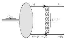
Figure 1: Bethe-Salpeter kernel for the two-parton system.

The dynamics of the system is described by the Bethe-Salpeter equation (BSE), which is explicitly invariant in any system and contains both a rest frame and a light front Schroedinger equations as special limits. In an explicit form, the BSE is written as (see Fig. 1)

$$i\chi_{ab}\left(p_{-},-p_{+}\right)=S_{ac}\left(p_{-}\right)\int\frac{d^{4}q}{(2\pi)^{4}}\tilde{A}_{ce,fd}\left(p_{-},q-p_{+}-p_{-},q-p_{+}\right)\,\chi_{ef}\left(q,\,q-p_{-}-p_{+}\right)S_{db}\left(-p_{+}\right),$$ (2)

where $p_{-}$ and $-p_{+}$ are momenta of the quark and antiquark respectively. In Eq. (2) $\tilde{A}_{ce,fd}$ denotes the 2-quark scattering amplitude. Recall that in this equation all ingredients are relativistic invariants and do not depend on the reference frame.

In a perturbative QCD, the propagator $S$ in the leading order should be replaced by the free quark propagator, and the vertex part $\tilde{A}$ should be replaced by a single-gluon exchange in the $t$-channel, so (2) simplifies to

$$i\chi\left(p_{-},-p_{+}\right)=S\left(p_{-}\right)\int\frac{d^{4}q}{(2\pi)^{4}}\frac{\gamma_{\mu}\chi\left(q,\,q-p_{-}-p_{+}\right)\gamma_{\mu}}{\left(q-p_{-}\right)^{2}+i0}S\left(-p_{+}\right),$$ (3)

where from now on we omit explicit Dirac indices. If we denote $p_{0}=P/2$, where $P$ is the momentum of the quarkonium, and define small deviations as $\delta p_{-}=p_{-}-p_{0},\quad-\delta p_{+}=-p_{+}-p_{0}$, after some well-known algebraic manipulations (see details in Appendix A), we may reduce (3) to

$$i\tilde{\chi}\left(p_{-},-p_{+}\right) = g\left(\delta p_{-}\right)g\left(-\delta p_{+}\right)\int\frac{d^{4}q}{(2\pi)^{4}}\,\frac{\tilde{\chi}\left(q,\,q-p_{-}-p_{+}\right)}{\left(q-p_{-}\right)^{2}+i0},$$ (4)

$$\tilde{\chi} \equiv \Lambda_{+}\gamma_{\mu}\chi\gamma_{\mu}\Lambda_{-}$$ (5)

Note that while $\tilde{\chi}$ is a matrix, equation (4) is a scalar equation (doesn’t mix components), and for this reason in what follows we may omit the spin structure of $\tilde{\chi}$ and treat it as a scalar function. Taking into account that the projection of the vector $q-p$ on $P$ is $\mathcal{O}\left(\alpha_{s}^{2}\right)$ (this corresponds to a generalization of the rest frame instantaneous approximation $k_{0}\approx 0$), after some algebra (see Appendix A) we can obtain a Schroedinger equation for the internal motion in the form

$$\left(i\partial_{\xi}+\frac{\partial_{\zeta}^{2}}{m_{q}}-\frac{p_{\perp}^{2}}{m_{q}}\right)\Psi\left(\zeta,r_{\perp}\right)=\tilde{V}\left(\zeta,r_{\perp}\right)\Psi\left(\zeta,r_{\perp}\right),$$ (6)

where we defined a wave function $\Psi$ as $\Psi=\int d\lambda\,\tilde{\chi}\left(q,\,q-P\right)_{{}_{\lambda=q\cdot P/M}},$ a potential $\tilde{V}$ is proportional to the trace of the gluon propagator, $\tilde{V}=g^{\mu\nu}\Pi_{\mu\nu}/4$, where $\Pi_{\mu\nu}$ is the gluon propagator, and the derivatives are defined as

$$\partial_{\xi} = -\left(\cosh\eta\partial_{0}+\sinh\eta\partial_{3}\right),$$ (7)

$$\partial_{\zeta} = -\left(\sinh\eta\partial_{0}+\cosh\eta\partial_{3}\right).$$ (8)

Here we introduced the shorthand notations $\eta=\ln\left(P^{+}/M\right)$, and $M$ for the mass of quarkonium. The relation of the effective potential $\tilde{V}$ to the rest frame potential will be discussed in the next section. Equation (6) provides a smooth interpolation between the rest frame ($\eta=0$) and light-front frame ($\eta\to\infty$). This equation can be also obtained from the pNRQCD lagrangian Brambilla:1999xf , which in a moving frame gets the form

$$L = \Psi_{S}^{\dagger}\left(i\partial_{\xi}+\frac{\partial_{\zeta}^{2}}{m_{q}}-\frac{p_{\perp}^{2}}{m_{q}}-V_{S}\right)\Psi_{S}+\Psi_{O}^{\dagger}\left(iD_{\xi}+\frac{\partial_{\zeta}^{2}}{m_{q}}-\frac{p_{\perp}^{2}}{m_{q}}-V_{O}\right)\Psi_{O}+$$

$$+ \frac{g}{m_{q}}\,V_{A}(r)\,\left(\Psi_{S}^{\dagger}r_{\perp}^{\mu}P^{\nu}F_{\mu\nu}\Psi_{O}+\Psi_{O}^{\dagger}r_{\perp}^{\mu}P^{\nu}F_{\mu\nu}\Psi_{S}\right)+$$

$$+ g\,\frac{V_{B}(r)}{2m_{q}}\,\left(\Psi_{O}^{\dagger}r_{\perp}^{\mu}P^{\nu}F_{\mu\nu}\Psi_{O}+\Psi_{O}^{\dagger}r_{\perp}^{\mu}P^{\nu}F_{\mu\nu}\Psi_{O}\right)-\frac{1}{4}F^{a,\mu\nu}F_{\mu\nu}^{a},$$

where $\Psi_{S}$ and $\Psi_{O}=\Psi_{O}^{a}t_{a}$ are the fields of the singlet and octet $\bar{q}q$-pair ($\Psi$ in (6) corresponds to $\Psi_{S}$ in (II)), $P_{\mu}$ is the momentum of the moving quarkonium, $D_{\xi}=\partial_{\xi}+ig[A_{\xi},\Psi_{O}]$, $A_{\mu}$ is the gauge field, and $V_{S}(r),\,V_{O}(s),\,V_{A}(r)$ and $V_{B}(r)$ are the potentials for singlet, octet diquarks and a transition matrix elements. While in pQCD they are given by well-known perturbative expressions, for a quarkonium propagating inside matter they become more complicated and get an absorptive part. A detailed study of the absorption mechanism is out of scope of this paper and will be presented elsewhere.

III Schroedinger equation from analyticity and unitarity

Notice that the single-gluon exchange in $t$-channel gives only a Coulomb term in the effective potential. As we have discussed in the introduction, such an approach can be justified only for very heavy quark states (say bottomonium), whereas for the $J/\Psi$ meson higher order corrections are essential. This fact manifests itself in the developed phenomenology  Digal:2005ht ; Eichten:1979ms ; Arafah:1983 ; Jacobs:1986 ; Gara:1990 ; Ikhdair:1992 ; Brambilla:1992 ; Fulcher:1993 ; Oh:2002 ; Blanck:2011 in the rest frame, in which an additional confining potential is added to one gluon exchange. This extra term is generated by nonperturbative interactions and introduced into the Bethe-Salpeter either as additional vector or scalar $t$-channel contribution (see e.g. Resag:1995 ).

Bearing this experience in mind, in this section we are going to obtain the Schroedinger equation for the non-relativistic system without using the explicit form of $\tilde{A}$ in Eq. (2). In the following discussion, it is convenient to write the amplitude $\chi$ as a function of the variables $s=\left(p_{-}-p_{+}\right)^{2}$and $p=p_{-}+p_{+}$ instead of parton momenta $p_{\pm}$ . The amplitude $\chi$ is analytic outside the real axis, so it can be represented as

$$\chi\left(p,\,M^{2}\right)=\frac{1}{2\pi}\int_{M^{2}}^{\infty}ds^{\prime}\,\frac{\mbox{Im}\,\chi(s^{\prime},\,p)}{s^{\prime}-M^{2}+i0},$$ (10)

where $M$ is the mass of the $\bar{q}q$ meson. The imaginary part of the amplitude $\chi$ can be evaluated directly from (2), using the unitarity constraints

$$\mbox{Im}\,\chi(s^{\prime},\,p)=\int d^{3}q\,\chi(s^{\prime},\,q)\,A_{2\to 2}\left(s^{\prime},\,\left(q-p\right)^{2}\right)\delta\left(s^{\prime}-\left(2q-p\right)^{2}\right)+\sum_{n=3}^{\infty}\chi_{1\to n}\bigotimes A_{n\to 2}$$ (11)

In this equation $A_{2\to 2}\left(s^{\prime},\,p-p^{\prime}\right)$ is the 2-particle scattering amplitude. If we neglect the contributions of higher Fock states ($n\geq 3$ in Eq. (11)) in the large-$m_{q}$ limit, we can re-write Eq. (10) and Eq. (11) in the following form

$$\chi\left(p,\,M^{2}\right)=\frac{1}{2\pi}\int d^{3}q\int_{M^{2}}^{\infty}ds^{\prime}\,\frac{\chi(s^{\prime},\,q)}{s^{\prime}-M^{2}+i0}\,A_{2\to 2}\left(s^{\prime},\,\left(q-p\right)^{2}\right)\delta\left(s^{\prime}-\left(2q-p\right)^{2}\right)+\mathcal{O}\left(\frac{\epsilon}{m_{G}}\right),$$ (12)

where $m_{G}\approx$ 1 GeV is the effective mass of gluon Graziani:1984cs . These estimates stem from the assumption that the second term in Eq. (11) has the same order of the magnitude as the first one, but its contribution starts to be essential for $s^{\prime}\,\geq\,(2m_{q}+m_{G})^{2}$. In the dispersion integral the first term shows the enhancement $\propto 1/(M\epsilon)$, while the second has the denominator $\propto 1/(M\,m_{g})$. It is difficult to make better estimates for accuracy of our calculation due to the lack of understanding of non-perturbative QCD.

It should be stressed that for very heavy quark-antiquark systems, at small distances the omitted terms have an additional suppression of the order of $\mathcal{O}(\alpha_{s}^{2}(m_{q}))$. In the case of realistic system such as the $J/\Psi$-meson we cannot use this smallness, and in order to evaluate the highly excited states in Eq. (11) we have to rely on models. It turns out that in phenomenological models for the $J/\Psi$-meson, a substantial contribution stems from the string-like potential. Indeed, $V_{{\rm eff}}(r_{J/\psi})-V_{{\rm pQCD}}(r_{J/\psi})\,\sim\,\sigma\langle r_{J/\psi}\rangle\,\approx\,0.4\,GeV$ for the string tension $\sigma=1\,GeV/fm$. Bearing this fact in mind we can estimate the contribution of the multi-particle states in the unitarity constraint, by comparing the mass of the next string excitation or, in other words, the mass of the next resonance on the $J/\Psi$ Reggeon trajectory with mass $M_{R}$. This contribution is suppressed by the parameter

$$Q=\frac{2\,M\epsilon}{M_{R}^{2}-M^{2}}.$$ (13)

The binding energy $\epsilon$ is a poorly defined object, since the mass of the heavy quark is scheme-dependent. For the case of charm quark, the estimates for the mass $m_{c}$ vary between 1.27 GeV and 1.8 GeV, so as an upper value estimate, we take $\epsilon_{{\rm max}}\approx 2M_{D}-M_{J/\psi}\approx 600\,{\rm MeV}$. Taking $M=M_{J/\psi}$ and $M_{R}=M_{\psi(3686)}$ PDG:2014 for the first excited state in a channel with $J/\psi$ quantum numbers, we get an upper limit for the parameter $Q_{{\rm max}}\approx 1/2$. In the small-$\epsilon$ approximation we may simplify (12) as

$$A_{2\to 2}\left(s^{\prime},\,\left(q-p\right)^{2}\right)\approx A_{2\to 2}\left(M^{2},\,\left(q-p\right)^{2}\right).$$ (14)

It should be mentioned that the assumption of Eq. (14) means that amplitude $A_{2\to 2}\left(s^{\prime},\,\left(q-p\right)^{2}\right)$ has no singularities related to the quark-antiquark state, and this amplitude can be viewed as a sum of quark-antiquark irreducible Feynman diagrams in QCD. Introducing a new function

$$\Psi(s,\,q)=\frac{\chi(s,\,q)}{s-M^{2}+i0},$$ (15)

we may rewrite (12) in the form

$$\left(p^{2}-M^{2}\right)\Psi(M^{2},\,p)=\frac{1}{2\pi}\int d^{3}q\,V(q-p)\Psi(M^{2},\,p).$$ (16)

In the instant form we may split the vector of relative motion $p$ into a part $p_{||}$ collinear to the quarkonium momentum $P$ and part $\delta p$ orthogonal to it. After some trivial algebra, (16) reduces to a simple Schroedinger equation (6). In the front form (16) reduces to the result obtained in Lepage:1980fj ,

$$M^{2}\Psi=\left(\frac{p_{\perp}^{2}+m_{q}^{2}}{x(1-x)}+\hat{U}\right)\Psi,\,$$ (17)

where $M$ is the mass of the meson, $q_{\perp}$ is the quark transverse momentum, $x$ is the light-front fraction of the longitudinal momentum of the quark, and $\hat{U}$ is the operator of the potential energy. In the heavy quark mass limit, there are two natural small parameters, $\mathcal{O}\left(\alpha_{s}\left(m_{q}\right)\right)$ and $\mathcal{O}\left(\Lambda_{{\rm QCD}}/m_{q}\right)$. Typical momenta of the quarks in a nonrelativistic system are of order $m_{q}\mathcal{O}\left(\alpha_{s}\left(m_{q}\right)\right)$, whereas the binding energy is $\epsilon\sim m_{q}\mathcal{O}\left(\alpha_{s}^{2}\left(m_{q}\right)\right)$. Taking into account that the light-front fraction $x\approx 1/2+\delta x$ where $\delta x\approx\mathcal{O}\left(\alpha_{s}\left(m_{q}\right)\right)$, we can see that (17) reduces to

$$\epsilon\Psi=\left(\frac{p_{\perp}^{2}}{m_{q}}+4m_{q}\,\delta x^{2}+\frac{1}{4m_{q}}\hat{U}\right)\Psi.$$ (18)

If we make a Fourier transformation of $\Psi$ to coordinate space according to

$$\phi\left(\zeta,\,r_{\perp}\right)=\int\frac{d\delta x\,d^{2}q_{\perp}}{(2\pi)^{2}}\Psi\left(x=\frac{1}{2}+\delta x,\,q_{\perp}\right)e^{2im_{q}\zeta\,\delta x-iq_{\perp}\cdot r_{\perp}},$$ (19)

where $\zeta$ is a parton separation along the $z^{-}$-axis, and $\phi$ satisfies the ordinary Schroedinger equation

$$\epsilon\phi\left(\zeta,\,r_{\perp}\right)=\left(\frac{-\Delta_{\perp}-\partial_{\zeta}^{2}}{m_{q}}+\hat{V}\right)\phi\left(\zeta,\,r_{\perp}\right),$$ (20)

where $\hat{V}=\hat{U}/(4m_{q})$. We would like to emphasize that in contrast to Gutsche:2014oua the potential $\hat{V}$ is local only in the coordinate space; in a LF frame the interaction has a form of a convolution

$$\hat{V}\phi\left(x,\,r_{\perp}\right)=\int V\left(x-x_{1},\,r_{\perp}\right)\phi\left(x_{1},\,r_{\perp}\right)dx_{1}.$$ (21)

The Green function of the internal motion in the infinite momentum frame satisfies an evolution equation

$$\frac{P^{+}}{M}\frac{\partial}{\partial x^{+}}\,G\left(x^{+},\zeta,\,r_{\perp};x_{1}^{+},\zeta_{1},r_{1,\perp}\right)=$$

$$= \frac{-\Delta_{\perp}-\partial_{\zeta}^{2}+m_{q}^{2}}{m_{q}}G\left(x^{+},\zeta,\,r_{\perp};x_{1}^{+},\zeta_{1},r_{1,\perp}\right)+\hat{V}G\left(x^{+},\zeta,\,r_{\perp};x_{1}^{+},\zeta_{1},r_{1,\perp}\right),$$

Finally, we would like to address how the light front and rest frame potentials are related to each other. From Eq. (14) we see that this amplitude is a function of only four-dimensional transfered momentum. As we can see from (6,16), a relation between the potentials in different frames can be extracted from the transformation of the gluon momentum $k=q-p$. In a rest frame, the vector $k$ has a negligible $k_{0}$ component (instantaneous approximation), so $k^{2}\approx-\vec{k}^{2}+\mathcal{O}\left(\alpha_{s}^{4}\right).$ In an infinite momentum frame, we may rewrite

$$k^{2}=\left(q-p\right)^{2}=\left(x-x_{1}\right)\left(\frac{m_{q}^{2}+p_{\perp}^{2}}{x}-\frac{m_{q}^{2}+q_{\perp}^{2}}{x_{1}}\right)-q_{\perp}^{2}\approx-\frac{m_{q}^{2}}{x\,x_{1}}\left(x-x_{1}\right)^{2}-q_{\perp}^{2}+\mathcal{O}\left(\alpha_{s}^{3}\right),$$ (23)

where light-front fractions are defined as $x=p^{+}/P^{+}$ and $x_{1}=q^{+}/P^{+}$. Note that $x-x_{1}\sim\mathcal{O}\left(q_{\perp}/m_{q}\right)$, so both terms are of the same order of smallness and the omission of the terms in a previous line is justified due to extra $\sim\mathcal{O}\left(q_{\perp}/m_{q}\right)$ suppression. After some lengthy but straightforward evaluations (see details in Appendix B) we may get for the interaction term in the infinite momentum frame

$$\left(\hat{U}\Psi\right)\left(x,\,r_{\perp}\right) = \int dx_{1}K\left(x,\,x_{1},\,r_{\perp}\right)\Psi\left(x_{1},\,r_{\perp}\right),$$ (24)

where the kernel

$$K\left(x,x_{1},r_{\perp}\right) = \int_{-\infty}^{\infty}\frac{dz}{2\pi}\,V\left(\sqrt{r_{\perp}^{2}+z^{2}}\right)\exp\left(2im_{q}\left(x-x_{1}\right)\,z\right).$$ (25)

In Figure 2 we compare the ground state ($J/\psi$) wave function evaluated from (III) with the one obtained with the phenomenological prescription Ivanov:2002kc . For the sake of definiteness, in both cases we used a rest frame potential from Karsch:1987pv . As we can see from the plots, for the symmetric configuration ($x\approx 0.5$) the wave function given by a prescription Ivanov:2002kc coincides within the accuracy of numerical evaluations with the eigenfunction of (III). However, for large-$x$ there is some disagreement between the two wave functions. This could be easily understood, taking into account that $x-1/2$ is a small $\mathcal{O}\left(\alpha_{s}\right)$ parameter which is neglected. The average width of the charmonium wave function is $\left\langle\left|x-\frac{1}{2}\right|\right\rangle\sim\langle p_{3}/2\,m_{q}\rangle\approx 0.2$, which signals that the relativistic effects, albeit small, are not completely negligible.

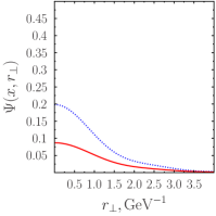
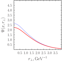
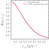
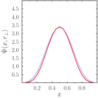
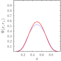
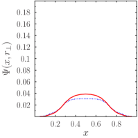
Figure 2: Comparison of the ground state wave functions evaluated with (III) (solid red line) and with a prescription from Ivanov:2002kc (dashed blue line). Upper row: $r_{\perp}$-dependence at fixed $x$. Lower row: $x$-dependence at fixed values of the parameter $r_{\perp}$.

IV Conclusions

In this paper we re-visit the problem of the wave function for the heavy quark-antiquark system in an arbitrary reference frame. In two regions: (i) $m_{q}\,\alpha_{S}\left(m_{q}\right)\,\gg\Lambda_{QCD}$ and (ii) $\epsilon/\Lambda_{QCD}\,\ll\,1$, we constructed a Schroedinger equation for the internal motion of $J/\psi$ moving in the laboratory frame with relativistic center-of-mass momentum (see Eq. (6)). In these cases, this equation reduces to the rest frame and infinite momentum Schroedinger equations, and thus gives a smooth interpolation between the two limits. We studied a relation between the rest frame and light-front potentials of quarkonium. We found that the two are related by a linear transformation (24), which corresponds to a large-$m_{q}$ limit of a nonlinear transformation in Trawinski:2014msa ; Gutsche:2014oua . The omitted terms are of higher order in $\mathcal{O}(\Lambda_{QCD}\Big{/}\left(\alpha_{s}\left(m_{q}\right)\right)$ and $\mathcal{O}\left(\epsilon\Big{/}\Lambda_{QCD}\right)$ and their inclusion is not justified in the two-parton approximation. We checked the phenomenological prescription Ivanov:2002kc and found that in the region $x\approx 0.5$, which is relevant for charmonium-related problems, it is well justified. Also, we got that in the infinite momentum frame a potential is given by a convolution (24,25) in light-front variable $x$, in contrast to what was found in Gutsche:2014oua .

Our results could be relevant for the description of the final state interactions of a wide class of processes including quarkonium production on nuclei or plasma. Besides, they could be extended to the description of final state interactions in the production of weakly bound systems, such as for example the deuteron.

Appendix A Derivation of the Schroedinger equation

The Bethe-Salpeter equation (BSE) has a form

$$i\chi_{ab}\left(p_{-},-p_{+}\right)=S_{ac}\left(p_{-}\right)\int\frac{d^{4}q}{(2\pi)^{4}}\tilde{A}_{ce,fd}\left(p_{-},q-p_{+}-p_{-},q-p_{+}\right)\chi_{ef}\left(q,\,q-p_{-}-p_{+}\right)S_{db}\left(-p_{+}\right),$$ (26)

where $p_{-}$ and $-p_{+}$ are the momenta of the quark and antiquark respectively, and we explicitly have shown lower Dirac/flavour indices. The Bethe-Salpeter amplitude defined as

$$\chi_{ab}\left(p_{1},\,p_{2}\right)=\int d^{4}x_{1}d^{4}x_{2}e^{i\left(p_{1}\cdot x_{1}-p_{2}\cdot x_{2}\right)}\langle 0|\psi_{a}\left(x_{1}\right)\bar{\psi}_{b}\left(x_{2}\right)|P\rangle$$

is not a wave function, but can be projected to a wave function integrating along some time-like curve. The propagator $S$ in leading order may be replaced by the free quark propagator, and the amplitude $\tilde{A}$ is dominated by a single-gluon exchange in the $t$-channel. Note however that single-gluon exchange produces just a Coulomb potential, whereas in realistic models we have also a string, so we assume that the gluon propagator has a form $\Pi_{\mu\nu}=g_{\mu\nu}\tilde{V},$ where $\tilde{V}$ is a Fourier image of the potential. In this case we may rewrite the equation (26) as

$$i\chi\left(p_{-},-p_{+}\right)=S\left(p_{-}\right)\int\frac{d^{4}q}{(2\pi)^{4}}\tilde{V}\left(q-p_{-}\right)\gamma_{\mu}\chi\left(q,\,q-p_{-}-p_{+}\right)\gamma_{\mu}S\left(-p_{+}\right),$$ (27)

Starting from this equation we omit the Dirac indices since we have a matrix identity. If we denote $p_{0}=P_{J/\Psi}/2$ and define small deviations as $\delta p_{-}=p_{-}-p_{0},\quad-\delta p_{+}=-p_{+}-p_{0}$, we may expect that a deviation of quark momenta from $p_{0}$ are small; the terms $\sim\delta p_{i}$ may be neglected in the numerator but should be retained in the denominator, so we get

$$S\left(p_{-}\right)=\frac{\hat{p}_{-}+m_{q}}{p_{-}^{2}-m_{q}^{2}+i0}\approx\frac{\hat{p}_{0}+m_{q}}{2m_{q}}\,\frac{1}{\frac{p_{0}\cdot\delta p_{-}}{m_{q}}-\frac{\delta\vec{p}_{-}^{2}}{2m_{q}}+i0}=\Lambda_{+}g\left(\delta p_{-}\right)$$ (28)

$$S\left(-p_{+}\right)=\frac{-\hat{p}_{+}+m_{q}}{p_{+}^{2}-m_{q}^{2}+i0}\approx\frac{\hat{p}_{0}-m_{q}}{2m_{q}}\,\frac{1}{-\frac{p_{0}\cdot\delta p_{+}}{m_{q}}-\frac{\delta\vec{p}_{+}^{2}}{2m_{q}}+i0}=\Lambda_{-}g\left(-\delta p_{+}\right)$$ (29)

where we introduced a shorthand notation for the projectors

$$\Lambda_{\pm}\equiv\frac{\hat{p}_{0}\pm m_{q}}{2m_{q}}$$

and a new function

$$g\left(\delta p\right)=\frac{1}{\frac{p_{0}\cdot\delta p}{m_{q}}-\frac{\delta\vec{p}^{2}}{2m_{q}}+i0}$$

Multiplying both parts of (27) by $\Lambda_{+}\gamma_{\nu}$ from the left and by $\gamma_{\nu}\Lambda_{-}$ from the right, after some manipulations with Dirac algebra, we get

$$i\tilde{\chi}\left(p_{-},-p_{+}\right) = g\left(\delta p_{-}\right)g\left(-\delta p_{+}\right)\int\frac{d^{4}q}{(2\pi)^{4}}\tilde{V}\left(q-p_{-}\right)\tilde{\chi}\left(q,\,q-p_{-}-p_{+}\right),$$ (30)

$$\tilde{\chi} \equiv \Lambda_{+}\gamma_{\mu}\chi\gamma_{\mu}\Lambda_{-}$$ (31)

In a moving system, a projection of the gluon momentum $q-p$ onto the direction of vector $p_{0}$ is $\mathcal{O}\left(\alpha_{s}^{2}\right)$, whereas all the other components are $\mathcal{O}\left(\alpha_{s}\right)$ so we may assume that the former can be neglected (it is a generalization of the instantaneous approximation in QCD). Let us introduce a vector

$$n_{0}=\left(\sinh\eta,\cosh\eta,\vec{0}_{\perp}\right).$$ (32)

where $\eta=\ln\left(P_{{\rm J/\psi}}^{+}/M_{{\rm J/\psi}}\right)$, and make a Sudakov decomposition of the vector $q$,

$$q=\lambda\frac{p_{0}}{m_{q}}+\tau n_{0}+q_{\perp}$$ (33)

In a rest frame the projection of the vector $q$ onto $p_{0}$ is suppressed as $\mathcal{O}\left(\alpha_{s}\right)$ compared to the other components, for this reason in a moving frame we expect that dependence on $\lambda$ should be negligible, i.e.

$$\tilde{V}=\tilde{V}\left(\tau,\,q_{\perp}\right)$$ (34)

We define a wave function as

$$\Psi(\tau,\,q_{\perp};\,P)=\int d\lambda\,\tilde{\chi}\left(q,\,q-P\right),$$

so (30) can be rewritten as

$$i\tilde{\chi}\left(p_{-},-p_{+}\right)=g\left(\delta p_{-}\right)g\left(-\delta p_{+}\right)\int\frac{d\tau dq_{\perp}}{(2\pi)^{4}}\tilde{V}\left(\tau-\tau_{-},q_{\perp}-p_{\perp}\right)\Psi(\tau,\,q_{\perp};\,P)$$ (35)

and $\tau_{-}=p_{-}\cdot n_{0}$. Defining $\lambda_{-}=p_{-}\cdot p_{0}/m_{q}$ and taking the integral over it in both parts of (35), we may get

$$\left(E-\frac{\tau^{2}}{m_{q}}-\frac{p_{\perp}^{2}}{m_{q}}\right)\Psi=\int\frac{d\tau d^{2}q_{\perp}}{\left(2\pi\right)^{3}}\tilde{V}\left(\tau-\tau_{-},q_{\perp}-p_{\perp}\right)\Psi(\tau,\,q_{\perp};\,P)$$ (36)

where $\tau=-p\cdot\bar{p}_{0}=-\sinh\eta\hat{p}_{0}+\cosh\eta\hat{p}_{3}$. In coordinate space, the corresponding wave function is

$$\Psi\left(\zeta,\,r_{\perp}\right)=\int\frac{d\tau d^{2}q_{\perp}}{(2\pi)^{3}}e^{i\zeta\tau+ir_{\perp}\cdot q_{\perp}}\Psi(\tau,\,q_{\perp};\,P)$$

where the parameter $\zeta$ is related to ordinary coordinates as

$$\zeta=x_{0}\sinh\eta-x_{3}\cosh\eta.$$

and has a meaning of $z$-coordinate in the $J/\Psi$ rest frame. The corresponding eigenvalue equation has a form of a Schroedinger equation in the rest frame,

$$\left(E+\frac{\partial_{\zeta}^{2}}{m_{q}}-\frac{p_{\perp}^{2}}{m_{q}}\right)\Psi\left(\zeta,r_{\perp}\right)=V\left(\zeta,r_{\perp}\right)\Psi\left(\zeta,r_{\perp}\right),$$ (37)

and thus guarantees a correct spectrum. For a nonstationary state, we have to replace $E\to i\partial_{\xi}$, where

$$\xi=x_{3}\sinh\eta-x_{0}\cosh\eta,$$

so the equation of motion is

$$\left(i\partial_{\xi}+\frac{\partial_{\zeta}^{2}}{m_{q}}-\frac{p_{\perp}^{2}}{m_{q}}\right)\Psi\left(\zeta,r_{\perp}\right)=V\left(\zeta,r_{\perp}\right)\Psi\left(\zeta,r_{\perp}\right),$$ (38)

Replacing

$$\partial_{\xi} = -\left(\cosh\eta\partial_{0}+\sinh\eta\partial_{3}\right),$$

$$\partial_{\zeta} = -\left(\sinh\eta\partial_{0}+\cosh\eta\partial_{3}\right),$$

in the lab-frame, we end up with the second order (w.r.t. time) equation

$$\left(-i\left(\cosh\eta\partial_{0}+\sinh\eta\partial_{3}\right)+\frac{\left(\sinh\eta\partial_{0}+\cosh\eta\partial_{3}\right)^{2}}{m_{q}}-\frac{p_{\perp}^{2}}{m_{q}}\right)\Psi=V\left(\zeta,r_{\perp}\right)\Psi.$$ (39)

Appendix B Derivation of (24,25)

As was discussed in section II, in order to find a relation between the rest frame and light front potentials, it is necessary to rewrite the gluon momentum in terms of the light-front components, as (23)

$$k^{2}=\left(q-p\right)^{2}=\left(x-x_{1}\right)\left(\frac{m_{q}^{2}+p_{\perp}^{2}}{x}-\frac{m_{q}^{2}+q_{\perp}^{2}}{x_{1}}\right)-q_{\perp}^{2}\approx-\frac{m_{q}^{2}}{x\,x_{1}}\left(x-x_{1}\right)^{2}-q_{\perp}^{2}+\mathcal{O}\left(\alpha_{s}^{3}\right).$$ (40)

where for the sake of brevity we introduced a notation $k=q-p$ for the gluon momentum. If $\Psi$ is the light-front wave function, and $\tilde{\Psi}\left(x_{1},p_{\perp}\right)$ is its Fourier transform over the transverse components, for the interaction term we get

$$\hat{U}\Psi = \int\frac{d^{2}p_{\perp}}{(2\pi)^{2}}e^{ip_{\perp}\cdot r_{\perp}}\int\frac{dx_{1}}{2\pi}\frac{d^{2}k_{\perp}}{(2\pi)^{2}}\tilde{V}\left(k_{\perp}^{2}+\frac{m_{q}^{2}}{x\,x_{1}}\left(x-x_{1}\right)^{2}\right)\tilde{\Psi}\left(x_{1},p_{\perp}-k_{\perp}\right)=$$

$$= \int\frac{d^{2}p_{\perp}}{(2\pi)^{2}}e^{ip_{\perp}\cdot r_{\perp}}\int\frac{dx_{1}}{2\pi}\frac{d^{2}k_{\perp}}{(2\pi)^{2}}d^{2}\rho_{\perp}e^{-i\left(p_{\perp}-k_{\perp}\right)\cdot\rho_{\perp}}\tilde{V}\left(k_{\perp}^{2}+\frac{m_{q}^{2}}{x\,x_{1}}\left(x-x_{1}\right)^{2}\right)\Psi\left(x_{1},\rho_{\perp}\right)=$$

$$= 2\int dx_{1}\frac{d^{2}k_{\perp}}{(2\pi)^{2}}r^{2}dr\,\frac{\sin\left(r\sqrt{k_{\perp}^{2}+\frac{m_{q}^{2}}{x\,x_{1}}\left(x-x_{1}\right)^{2}}\right)}{r\sqrt{k_{\perp}^{2}+\frac{m_{q}^{2}}{x\,x_{1}}\left(x-x_{1}\right)^{2}}}V(r)e^{-ik_{\perp}\cdot r_{\perp}}\Psi\left(x_{1},r_{\perp}\right)=$$

$$= \int dx_{1}K\left(x,x_{1},r_{\perp}\right)\Psi\left(x_{1},r_{\perp}\right),$$

where we introduced a kernel $K$ defined as

$$K\left(x,x_{1},r_{\perp}\right) = 2\int\frac{k_{\perp}dk_{\perp}}{2\pi}dr\,\frac{r\,\sin\left(r\sqrt{k_{\perp}^{2}+\frac{m_{q}^{2}}{x\,x_{1}}\left(x-x_{1}\right)^{2}}\right)}{\sqrt{k_{\perp}^{2}+\frac{m_{q}^{2}}{x\,x_{1}}\left(x-x_{1}\right)^{2}}}V(r)J_{0}\left(k_{\perp}r_{\perp}\right)$$ (42)

In the nonrelativistic limit we may approximate $x\,x_{1}\approx 1/4$ and simplify the kernel (42) to

$$K\left(x,x_{1},r_{\perp}\right)\approx 2\int_{0}^{\infty}dr\,r\,V(r)\int_{0}^{\infty}\frac{k_{\perp}\,dk_{\perp}}{2\pi}\,\frac{\sin\left(r\sqrt{k_{\perp}^{2}+4m_{q}^{2}\left(x-x_{1}\right)^{2}}\right)}{\sqrt{k_{\perp}^{2}+4m_{q}^{2}\left(x-x_{1}\right)^{2}}}J_{0}\left(r_{\perp}k_{\perp}\right).$$ (43)

The integral over $k_{\perp}$may be taken introducing a new variable $\kappa=\sqrt{k_{\perp}^{2}+4m_{q}^{2}\left(x-x_{1}\right)^{2}}$ and using Integral $6.677.1$ from Ryzhik, Gradstein, as

$$K\left(x,x_{1},r_{\perp}\right)\approx 2\int_{0}^{\infty}dr\,r\,V(r)\int_{2m_{q}\left|x-x_{1}\right|}^{\infty}\frac{d\kappa_{\perp}}{2\pi}\,\sin\left(r\kappa\right)J_{0}\left(r_{\perp}\sqrt{\kappa^{2}-4m_{q}^{2}\left(x-x_{1}\right)^{2}}\right)=$$ (44)

$$= 2\int_{0}^{\infty}dr\,r\,V(r)\times\frac{\theta\left(r>r_{\perp}\right)}{2\pi}\frac{\cos\left(2m_{q}\left|x-x_{1}\right|\sqrt{r^{2}-r_{\perp}^{2}}\right)}{\sqrt{r^{2}-r_{\perp}^{2}}}=$$ (45)

$$= \frac{1}{\pi}\int_{r_{\perp}}^{\infty}dr\,r\,V(r)\frac{\cos\left(2m_{q}\left|x-x_{1}\right|\sqrt{r^{2}-r_{\perp}^{2}}\right)}{\sqrt{r^{2}-r_{\perp}^{2}}}.$$ (46)

Now again change a variable of integration, $z=\sqrt{r^{2}-r_{\perp}^{2}}$, $dz=rdr/\sqrt{r^{2}-r_{\perp}^{2}}$, $z\in(0,\infty)$, $r=\sqrt{r_{\perp}^{2}+z^{2}}$, so we get a result in a very clear and elegant form:

$$\Rightarrow K\left(x,x_{1},r_{\perp}\right)=\frac{1}{\pi}\int_{0}^{\infty}dz\,V\left(\sqrt{r_{\perp}^{2}+z^{2}}\right)\cos\left(2m_{q}\left|x-x_{1}\right|z\right),$$ (47)

$$\left(\hat{U}\Psi\right)\left(x,r_{\perp}\right) = \int dx_{1}K\left(x,x_{1},r_{\perp}\right)\Psi\left(x_{1},r_{\perp}\right).$$ (48)

Notice that since $\cos(...)$ is an even function, we may omit an absolute value sign, $|x-x_{1}|\to x-x_{1}$. Also, using symmetry w.r.t. $z\to-z$, we can extend the integration region from $-\infty$ to $+\infty$, adding an extra prefactor $1/2$, and also adding $i\int_{-\infty}^{+\infty}dz\sin\left(2m\left|x-x_{1}\right|z\right)$, which after integration of a symmetric potential yields zero, so the final result for the kernel $K$ may be cast into an equivalent form

$$K\left(x,x_{1},r_{\perp}\right)=\int_{-\infty}^{\infty}\frac{dz}{2\pi}\,V\left(\sqrt{r_{\perp}^{2}+z^{2}}\right)\exp\left(2im_{q}\left(x-x_{1}\right)z\right).$$ (49)

References

• (1) G. P. Lepage and S. J. Brodsky, Phys. Rev. D 22, 2157 (1980).
• (2) S. J. Brodsky and J.-P. Lansberg, Phys. Rev. D 81, 051502 (2010).
• (3) S. J. Brodsky, H. C. Pauli and S. S. Pinsky, Phys. Rept. 301, 299 (1998) [hep-ph/9705477].
• (4) Y. P. Ivanov, B. Z. Kopeliovich, A. V. Tarasov and J. Hufner, Phys. Rev. C 66, 024903 (2002) [hep-ph/0202216].
• (5) B. Kopeliovich, A. Tarasov and J. Hüfner, Nucl. Phys. A 696, 669 (2001).
• (6) B. Z. Kopeliovich and A. V. Tarasov, Nucl. Phys. A 710, 180 (2002) [hep-ph/0205151].
• (7) B. Z. Kopeliovich, I. K. Potashnikova, I. Schmidt and M. Siddikov, Nucl. Phys. A (2014) [arXiv:1407.8080 [nucl-th]].
• (8) B. Z. Kopeliovich, I. K. Potashnikova, I. Schmidt and M. Siddikov, arXiv:1409.5147 [hep-ph].
• (9) J. G. Korner and G. Thompson, Phys. Lett. B 264, 185 (1991).
• (10) N. Brambilla, A. Pineda, J. Soto and A. Vairo, Nucl. Phys. B 566, 275 (2000) [hep-ph/9907240].
• (11) M. Arafah, R. Bhandari, B. Ram, Lett. Nuov. Cim. 38, 305 (1983).
• (12) S. Jacobs, M. G. Olsson and C. Suchyta, Phys. Rev. D 33, 3338 (1986).
• (13) A. Gara, B. Durand and L. Durand, Phys. Rev. D 42, 1651.
• (14) S. M. Ikhdair, R. Sever, Z. Phys. C 56, 155 (1992).
• (15) N. Brambilla and G. M. Prosperi, Phys. Rev. D 46, 1096 (1992).
• (16) L. P. Fulcher, Z. Chen, and K. C. Yeong, Phys. Rev. D 47, 4122 (1993).
• (17) Y. Oh, S.  Kim, and S. H. Lee, Phys. Rev. C 65, 067901 (2002).
• (18) M. Blank and A. Krassnigg, Phys. Rev. D 84, 096014 (2011).
• (19) M. Beneke, Y. Kiyo and K. Schuller, Nucl. Phys. B 714 (2005) 67 [hep-ph/0501289].
• (20) N. Brambilla et al. [Quarkonium Working Group Collaboration], hep-ph/0412158.
• (21) N. Brambilla, M. A. Escobedo, J. Ghiglieri, J. Soto and A. Vairo, JHEP 1009, 038 (2010) [arXiv:1007.4156 [hep-ph]].
• (22) T. Matsui and H. Satz, Phys. Lett. B 178, 416 (1986).
• (23) S. Digal, O. Kaczmarek, F. Karsch and H. Satz, Eur. Phys. J. C 43 (2005) 71 [hep-ph/0505193].
• (24) E. Eichten, K. Gottfried, T. Kinoshita, K. D. Lane and T. -M. Yan, Phys. Rev. D 21, 203 (1980).
• (25) O. Kaczmarek, S. Ejiri, F. Karsch, E. Laermann and F. Zantow, Prog. Theor. Phys. Suppl.  153, 287 (2004) [hep-lat/0312015].
• (26) O. Kaczmarek, F. Karsch, F. Zantow and P. Petreczky, Phys. Rev. D 70, 074505 (2004) [Erratum-ibid. D 72, 059903 (2005)] [hep-lat/0406036].
• (27) O. Kaczmarek, “Recent Developments in Lattice Studies for Quarkonia,” arXiv:1208.4075 [hep-lat].
• (28) F. Karsch, M. T. Mehr and H. Satz, Z. Phys. C 37, 617 (1988).
• (29) F. Karsch, D. Kharzeev and H. Satz, Phys. Lett. B 637, 75 (2006).
• (30) M. Bedjidian, D. Blaschke, G. T. Bodwin, N. Carrer, B. Cole, P. Crochet, A. Dainese and A. Deandrea et al., hep-ph/0311048.
• (31) B. Z. Kopeliovich, Nucl. Phys. A 854, 187 (2011).
• (32) A. P. Trawiński, S. ła. D. Głazek, S. J. Brodsky, G. F. de Téramond and H. G. Dosch, arXiv:1403.5651 [hep-ph].
• (33) T. Gutsche, V. E. Lyubovitskij, I. Schmidt and A. Vega, Phys. Rev. D 90, no. 9, 096007 (2014) [arXiv:1410.3738 [hep-ph]].
• (34) J. Carbonell and V. A. Karmanov, arXiv:1408.3761 [hep-ph].
• (35) J. Resag, C.R. Münz, Nuclear Physics A 590, 735 (1995)
• (36) K.A. Olive et al. (Particle Data Group), Chin. Phys. C, 38, 090001 (2014).
• (37) F. R. Graziani, Z. Phys. C 33, 397 (1987).