Two–photon lasing by a superconducting qubit

Abstract

We study the response of a magnetic-field-driven superconducting qubit strongly coupled to a superconducting coplanar waveguide resonator. We observed a strong amplification/damping of a probing signal at different resonance points corresponding to a one and two-photon emission/absorption. The sign of the detuning between the qubit frequency and the probe determines whether amplification or damping is observed. The larger blue detuned driving leads to two-photon lasing while the larger red detuning cools the resonator. Our experimental results are in good agreement with the theoretical model of qubit lasing and cooling at the Rabi frequency.

Motivated by the first experiment demonstrating the energy exchange between a strongly driven superconducting qubit and a resonator at the Rabi frequency $\Omega_{R}$Il’ichev et al. (2003), Hauss et al.Hauss et al. (2008) elaborated a theoretical model to quantify this phenomenon. Their model predicts large resonant effects for the one- and two-photon resonance conditions $\Omega_{R}=\omega_{r}-g_{3}\bar{n}$ and $\Omega_{R}=2\omega_{r}-g_{3}\bar{n}$, where $\omega_{r}$ is the fundamental frequency of the resonator, $g_{3}$ is the effective coupling energy, and $\bar{n}$ is the average number of photons in the resonator at frequency $\omega_{r}$. Depending on the detuning between the driving frequency $\omega_{d}$ and the qubit eigenfrequency $\omega_{q}$, either a lasing behavior (blue detuning $\omega_{d}$ - $\omega_{q}>0$) of the oscillator can be realized or the qubit can cool the oscillator (red detuning $\omega_{d}$ - $\omega_{q}<0$). According to the theory, one-photon lasing/cooling effects vanish at the symmetry (degeneracy) point of the qubit. However, the two-photon processes persist at the symmetry point where the qubit-oscillator coupling is quadratic and decoherence effects are minimized. There, the system realizes a “single-atom-two-photon laser”. Note a similar two-photon lasing by a quantum dot in a microcavity, which was investigated theoretically in Ref. del Valle et al., 2010.

Experimentally, a single qubit one-photon lasing was demonstrated by the NEC group Astafiev et al. (2007). Here, a single charge qubit was used and a population inversion was provided by single-electron tunneling. Later on, the amplification/deamplification of a transmitted signal trough a coplanar waveguide resonator was achieved by a strongly driven single flux qubit.Oelsner et al. (2013) However, the two-photon lasing has not been experimentally demonstrated yet. In this paper, we demonstrate the two-photon lasing, as well as considerable enhancement of one-photon lasing of a superconducting qubit by one order of magnitude in comparison with Ref. Oelsner et al., 2013. This enhancement was achieved by a much stronger coupling of the superconducting qubit to the resonator.

The lasing effect was investigated by making use of a standard arrangement: a superconducting qubit placed in the middle of a niobium $\lambda/2$ coplanar waveguide resonator. The latter was fabricated by conventional sputtering and dry etching of a 150-nm-thick niobium film. The patterning uses an electron beam lithography and a CF₄ ion etching process. The aluminum qubits were fabricated by the shadow evaporation technique. The coupling between the qubit and the resonator was implemented by a shared Josephson junction (Fig. 1). The dimensions of the qubit’s Josephson junctions are $0.2\times 0.3~{}\mu$m², $0.2\times 0.2~{}\mu$m² and $0.2\times 0.3~{}\mu$m², the critical current density is about 200 A/cm², and the area of the qubit loop is $5\times 4.5~{}\mu$m². The resonance frequency and the quality factor of the resonator’s fundamental mode taken for a weak probing (-141 dBm) are $\omega_{r}=2\pi\times 2.482$ GHz, $Q_{0}=18\;000$. The same parameters of the third harmonics taken at the same power are $\omega_{r3}=2\pi\times 7.446$ GHz, $Q_{3}=3750$. These values were determined from the transmission spectra of the coplanar waveguide resonator.

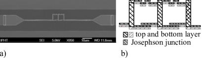
Figure 1: a) Scanning electron microscope image of the qubits incorporated into the coplanar waveguide resonator. b) Detailed scheme of the qubits. The qubits share a Josephson junction with each other as well as with the resonator.

In practice, we measured a two-qubit sample which represents a unit cell of a one-dimensional array of ferromagnetically coupled qubits exhibiting a large Kerr nonlinearity.Rehák et al. (2014) However, by applying a certain energy bias, one qubit can be set to a localized state, while the second is in the vicinity of its degeneracy point. This way, we can measure the qubits separately to reconstruct their parametersIl’ichev et al. (2004), and the dynamics of the system is defined by a single qubit only. Therefore, to describe our findings, we will use the one-qubit model elaborated in Ref. Hauss et al., 2008, in which the corresponding Hamiltonian reads in the flux basis of the qubit:

$$H = -\frac{1}{2}\epsilon\sigma_{z}-\frac{1}{2}\Delta\sigma_{x}-\hbar\Omega_{R0}\cos(\omega_{d}t)\sigma_{z}$$

$$+ \hbar\omega_{r}a^{\dagger}a+g\sigma_{z}(a^{\dagger}+a)$$

where $\Delta$ is the energy level separation of the two level system at zero energy bias $\epsilon=0$, $\Omega_{R0}$ is the driving amplitude of the applied microwave magnetic flux with frequency $\omega_{d}$, and $g$ is the coupling energy between the qubit and the resonator. The coupling energy scales with the ratio of the magnitude of the persistent current in the qubit $I_{q}$ and the critical current of the coupling Josephson junction $I_{c0}$ as

$$g\equiv\hbar\omega_{g}=\frac{\hbar\omega_{r}}{2\pi}\frac{I_{q}}{I_{c0}}\sqrt{\frac{1}{G_{0}Z_{r}}}$$ (2)

where $Z_{r}=50\Omega$ is the wave impedance of the coplanar waveguide resonator and $G_{0}\equiv 2e^{2}/h$ is the quantum conductance.

This Hamiltonian can be transformed by the Schrieffer-Wolff transformation $U=\exp(iS)$ with the generator $S=(g/\hbar\omega_{q})\cos\eta(a+a^{\dagger})\sigma_{y}$ and a rotating wave approximation $U_{R}=\exp(-i\omega_{d}\sigma_{z}t/2)$ to the HamiltonianHauss et al. (2008)

$$\tilde{H} = \hbar\omega_{r}a^{\dagger}a+\frac{1}{2}\hbar\Omega_{R}\sigma_{z}$$

$$+ g\sin\eta[\sin\beta\sigma_{z}-\cos\beta\sigma_{x}](a+a^{\dagger})$$

$$- \frac{g^{2}}{\hbar\omega_{q}}\cos^{2}\eta[\sin\beta\sigma_{z}-\cos\beta\sigma_{x}](a+a^{\dagger})^{2}$$

Here, $\hbar\omega_{q}=\sqrt{\epsilon^{2}+\Delta^{2}}$, $\Omega_{R}=\sqrt{\Omega_{R0}^{2}\cos^{2}\eta+\delta\omega^{2}}$, $\tan\eta=\epsilon/\Delta$, $\tan\beta=\delta\omega/(\Omega_{R0}\cos\eta)$ and $\delta\omega=\omega_{d}-\omega_{q}$. The transmission of the resonator

$$t\propto\langle a\rangle$$ (3)

where

$$\langle a\rangle=tr(\tilde{\rho}a)$$ (4)

was calculated numerically by the quantum toolbox Qutip,Johansson et al. (2013) solving the Liouville equation for the density matrix of the system in the rotating frame

$$\dot{\tilde{\rho}}=-\frac{i}{\hbar}\left[\tilde{H},\tilde{\rho}\right]+\tilde{L}_{q}\tilde{\rho}+\tilde{L}_{r}\tilde{\rho}$$ (5)

where $\tilde{L}_{q}$ and $\tilde{L}_{r}$ are Lindblad superoperators

$$\tilde{L}_{q}\tilde{\rho} = \frac{\tilde{\Gamma}_{\downarrow}}{2}(2\sigma_{-}\tilde{\rho}\sigma_{+}-\tilde{\rho}\sigma_{+}\sigma_{-}-\sigma_{+}\sigma_{-}\tilde{\rho})$$ (6)

$$+ \frac{\tilde{\Gamma}_{\uparrow}}{2}(2\sigma_{+}\tilde{\rho}\sigma_{-}-\tilde{\rho}\sigma_{-}\sigma_{+}-\sigma_{-}\sigma_{+}\tilde{\rho})$$

$$+ \frac{\tilde{\Gamma}_{\varphi}}{2}(\sigma_{z}\tilde{\rho}\sigma_{z}-\tilde{\rho}),$$

$$\tilde{L}_{r}\tilde{\rho} = \frac{\kappa}{2}(N_{th}+1)(2a\tilde{\rho}a^{\dagger}-\tilde{\rho}a^{\dagger}a-a^{\dagger}a\tilde{\rho})$$ (7)

$$+ \frac{\kappa}{2}N_{th}(2a^{\dagger}\tilde{\rho}a-aa^{\dagger}\tilde{\rho}-\tilde{\rho}aa^{\dagger}).$$

Here $N_{th}=1/\,[exp(\hbar\omega_{T}/k_{B}T)-1]$ is the thermal distribution function of photons in the resonator, $\kappa$ is resonator loss rate, $\tilde{\Gamma}_{\downarrow,\uparrow}$ and $\tilde{\Gamma}_{\varphi}$ are the relaxation, excitation and dephasing rates in the rotating frame derived in Ref. Hauss et al., 2008

$$\tilde{\Gamma}_{\uparrow,\downarrow} = \frac{\Gamma_{0}}{4}\cos^{2}\eta(1\pm\sin\beta)^{2}+\frac{\Gamma_{\varphi}}{2}\sin^{2}\eta\cos^{2}\beta$$

$$\tilde{\Gamma}_{\varphi} = \frac{\Gamma_{0}}{2}\cos^{2}\eta\cos^{2}\beta+\Gamma_{\varphi}\sin^{2}\eta\sin^{2}\beta$$ (8)

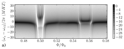
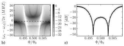
Figure 2: (a) Resonator transmission as a function of the magnetic flux and the detuning of the resonator from the third harmonic resonance frequency $\omega_{r3}/2\pi$. The anticrossings of qubit A and B are separated by a magnetic flux of about $55\times 10^{-3}\Phi_{0}$. (b) Close view of the transmission in the vicinity of the left qubit’s (A) degeneracy point and (c) the cut of the transmission map along the dashed line in (b). The crosses are experimental data and the solid line is a theoretical curve calculated from Eq. 9.

The qubit parameters used for the numerical calculations were determined independently from the transmission of the resonator $t$ coupled to the undriven qubit. For a weak microwave signal with frequency $\omega_{s}$, the transmission can be expressed in simple form Omelyanchouk et al. (2010)

$$t=-i\dfrac{\kappa_{ext}}{2}\dfrac{\delta\omega_{q}+i\gamma}{\omega_{g}^{2}\cos^{2}\eta-\left(\delta\omega_{r}+i\kappa/2\right)\left(\delta\omega_{q}+i\gamma\right)}$$ (9)

where $\delta\omega_{q}=\omega_{q}-\omega_{s}$, $\delta\omega_{r}=\omega_{r}-\omega_{s}$, $\kappa_{ext}$ is the external loss rate of the resonator and $\gamma$ is the qubit decoherence rate. The experimental data was fitted by Eq.9 (see Fig. 2) and the qubit parameters obtained from the fitting procedure are given in the table 1.

Qubit	Ip	$\Delta$/2$\pi$	g/2$\pi$	$\gamma$/2$\pi$
	(nA)	(GHz)	(MHz)	(MHz)
A	208	6.39	109	15
B	138	5.28	77	20

Table 1: Qubit parameters determined from the fitting procedure.

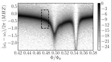
Figure 3: a) Resonator transmission in dB units as a function of the magnetic flux and the detuning of the resonator from the resonance frequency 2.482 GHz.

We have investigated the stimulated emission effect observed when strongly driving the system at a frequency $\omega_{d}/2\pi=9\omega_{r}/2\pi=22.338$ GHz for qubit A. The resonator transmission was measured by a network analyzer at resonance $\omega_{r}$ for magnetic fluxes marked by the black rectangular area in Fig. 3 and is shown in Fig. 4a.

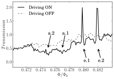
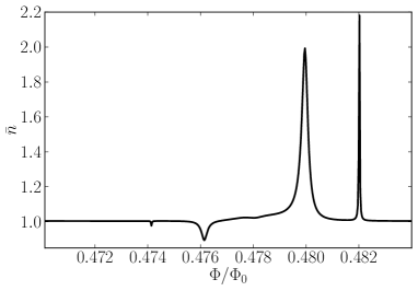
Figure 4: Transmission of the resonator at fixed frequency $\omega_{s}/2\pi$ for a driving signal with frequency $\omega_{d}/2\pi=9\omega_{r}/2\pi=22.338$ GHz and power $p_{d}=-102$ dBm for the driving switched off and on (a). Regions $e.1$, $e.2$ and $a.1$, $a.2$ exhibit amplification and attenuation of the signal, respectively. Panel (b) shows the simulated average photon number in the resonator obtained for the qubit parameters.

At a driving power $P_{d}=-103$ dBm, two emission peaks ($e.1$, $e.2$) accompanied by two attenuation dips ($a.1$, $a.2$) appear in the transmission spectra. The increase of the transmission is accompanied by a narrowing of the resonance curve. The one-photon ($a.1$, $e.1$) and two photon ($a.2$, $e.2$) processes are enhanced at resonance with the Rabi frequency of the qubit $\Omega_{R}=\omega_{r}-g_{3}\bar{n}$ and $\Omega_{R}=2\omega_{r}-g_{3}\bar{n}$, respectively. These results are in good agreement with the theoretical modelHauss et al. (2008) described above for parameters given in Table 1. By a strong coupling of the qubit to the resonator, we have achieved a considerable enhancement of the lasing, nearly one order of magnitude, in comparison with the results presented in Ref. Oelsner et al., 2013. Further improvement is possible by increasing the relaxation rate of the qubit, for instance, by placing a gold resistor close to the qubit loop.

To conclude, we have experimentally demonstrated single-qubit one-photon and two-photon lasing. The experimental results are in good agreement with the theoretical model developed by Hauss et al.Hauss et al. (2008) The considerable enhancement of lasing effect was achieved by stronger coupling of the superconducting qubit to the resonator, and theoretical calculations show that it can be enhanced further by increasing the relaxation rate of the qubit. Such improvement could enable to observe even higher-order processes analysed in Ref. Shevchenko et al., 2014.

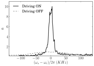
Figure 5: Resonance curve of the resonator at driving switched off (solid line) and on (dashed line) with frequency $\omega_{d}/2\pi=9\omega_{r}/2\pi=22.338$ GHz and power $p_{d}=-101$ dBm in region $e.1$. The amplitude increases by a factor of $\sim 9$ and bandwidth is reduced by factor of 10.

The research leading to these results has received funding from the European Community’s Seventh Framework Programme (FP7/2007-2013) under Grant No. 270843 (iQIT) and APVV-DO7RP003211. This work was also supported by the Slovak Research and Development Agency under the contract APVV-0515-10 and APVV-0808-12(former projects No. VVCE-0058-07, APVV-0432-07) and LPP-0159-09. The authors gratefully acknowledge the financial support of the EU through the ERDF OP R$\&$D, Project CE QUTE $\&$ metaQUTE, ITMS: 24240120032 and CE SAS QUTE. EI acknowledges partial support of Russian Ministry of Education and Science, in the framework of state assignment 8.337.2014/K.

References

- Il’ichev et al. (2003) E. Il’ichev, N. Oukhanski, A. Izmalkov, Th.Wagner, M. Grajcar, H.-G. Meyer, A. Smirnov, A. Maassen van den Brink, M. H. S. Amin, and A. Zagoskin, Phys. Rev. Lett. 91, 097906 (2003).
- Hauss et al. (2008) J. Hauss, A. Fedorov, C. Hutter, A. Shnirman, and G. Schön, Physical Review Letters 100, 037003 (2008).
- del Valle et al. (2010) E. del Valle, S. Zippilli, F. P. Laussy, A. Gonzalez-Tudela, G. Morigi, and C. Tejedor, Phys. Rev. B 81, 035302 (2010).
- Astafiev et al. (2007) O. Astafiev, K. Inomata, A. O. Niskanen, T. Yamamoto, Y. A. Pashkin, Y. Nakamura, and J. S. Tsai, Nature 449, 588 (2007).
- Oelsner et al. (2013) G. Oelsner, P. Macha, O. V. Astafiev, E. Il’ichev, M. Grajcar, U. Hübner, B. I. Ivanov, P. Neilinger, and H.-G. Meyer, Phys. Rev. Lett. 110, 053602 (2013).
- Rehák et al. (2014) M. Rehák, P. Neilinger, M. Grajcar, G. Oelsner, U. Hübner, E. Il’ichev, and H.-G. Meyer, Applied Physics Letters 104, 162604 (2014).
- Il’ichev et al. (2004) E. Il’ichev, N. Oukhanski, T. Wagner, H.-G. Meyer, A. Smirnov, M. Grajcar, A. Izmalkov, D. Born, W. Krech, and A. Zagoskin, Low Temp. Phys. 30, 620 (2004).
- Johansson et al. (2013) J. Johansson, P. Nation, and F. Nori, Computer Physics Communications 184, 1234 (2013).
- Omelyanchouk et al. (2010) A. N. Omelyanchouk, S. N. Shevchenko, Y. S. Greenberg, O. Astafiev, and E. Il’ichev, Low Temperature Physics 36, 893 (2010).
- Shevchenko et al. (2014) S. N. Shevchenko, G. Oelsner, Y. S. Greenberg, P. Macha, D. S. Karpov, M. Grajcar, U. Hübner, A. N. Omelyanchouk, and E. Il’ichev, Phys. Rev. B 89, 184504 (2014).