Polarization rotation by an rf-SQUID metasurface

Abstract

We study the transmission and reflection of a plane electromagnetic wave through a two dimensional array of rf-SQUIDs. The basic equations describing the amplitudes of the magnetic field and current in the split-ring resonators are developed. These yield in the linear approximation the reflection and transmission coefficients. The polarization of the reflected wave is independent of the frequency of the incident wave and of its polarization; it is defined only by the orientation of the split-ring. The reflection and transmission coefficients have a strong resonance that is determined by the parameters of the rf-SQUID; its strength depends essentially on the incident angle.

I Introduction

Recently a layer of metamaterial containing specially etched designs, referred to as metasurfaces, was used to induce a phase gradient in an incident electromagnetic waveygk11 . This leads to a generalized Snell’s law and the control of the transverse structure of the wave frontygk11 . This study was done in the optical domain, it then was extended to microwaves by Shalaev et al shalaev12 . The phase gradient is due to a plasmon resonance between the electromagnetic wave and the designs etched on the surface. These have to be adapted for each frequency domain and are fixed by construction.

It would be useful to have a system whose response could be changed over a significant range of frequencies. Such a device exists, it is a split-ring Josephson resonator (rf-SQUID) Lazarides:07a ; Lazarides:07b ; Lazarides:09 ; Maim:Gabi:10 . The rf-SQUIDs as basic elements of quantum metamaterials were discussed in Chunguang:06 ; Anlage:11 ; Trepanier:11 ; cgm12 . In the experimental study Ustinov:13 , it was shown that one can tune the resonance frequency of these devices. It should be pointed that this system has a discrete energy spectrum and a large magnetic momentum cgm12 . Then the energy of interaction with an external field can be of the order of the transition energy between neighboring energy states.

In this article we show that a film of properly oriented rf-SQUID controls the polarization of a wave reflecting on the meta-surface. This is similar to a Faraday effect; the wave is strongly reoriented at the resonance. We determine the parameters of the reflected and transmitted waves in the linear approximation. The reflection and transmission coefficients depend on the frequency and on the stationary state of the system. In that sense, the device is active, its parameters can be modified.

II The model

We consider a plane wave normally incident on a layer of rf-SQUIDs as shown in Fig.1. All the rings in the layer are oriented in the same direction given by the normal vector $\mathbf{n}$. The interaction of the individual rf-SQUID with the electromagnetic field is determined by the magnetic flux through the split ring. Therefore the orientation of the rf-SQUID controls the parameters of the transmitted and reflected waves. This orientation is characterized by the angle $\theta$ between the magnetic component $\mathbf{H}$ and the normal $\mathbf{n}$ to the split ring. We assume the same homogeneous dielectric layers above and below the the film. The dielectric permittivity of this medium is $\varepsilon$. The model describing the interaction of electromagnetic field with the system of rf-SQUIDs is based on Maxwell’s equations and the equation for the response of the rf-SQUIDs:

$$\nabla\times\mathbf{E}=-(\mu_{0}\mathbf{H}+\mathbf{M})_{t},$$ (1)

$$\nabla\times\mathbf{H}=\varepsilon_{0}\varepsilon\mathbf{E}_{t},$$ (2)

$$\nabla\cdot\mathbf{D}=0,\quad\nabla\cdot\mathbf{B}=0.$$ (3)

The magnetization $\mathbf{M}$ in the equation (1) is localized in the array whose thickness is much smaller than the wavelength $\lambda$. Therefore the magnetization can be written as follows:

$$\mathbf{M}(t,\mathbf{r})=\sum_{a}\mathbf{m}_{a}(t)\delta(z)\approx\mathbf{m}(t)n_{r}l\delta(z),$$ (4)

where $\mathbf{m}_{a}(t)$ are individual rf-SQUIDs magnetizations, $l<<\lambda$ is the film thickness, $n_{r}$ is the density of rf-SQUIDS resonators and $\mathbf{m}(t)$ is the magnetic moment of the ring Maim:Gabi:10 .

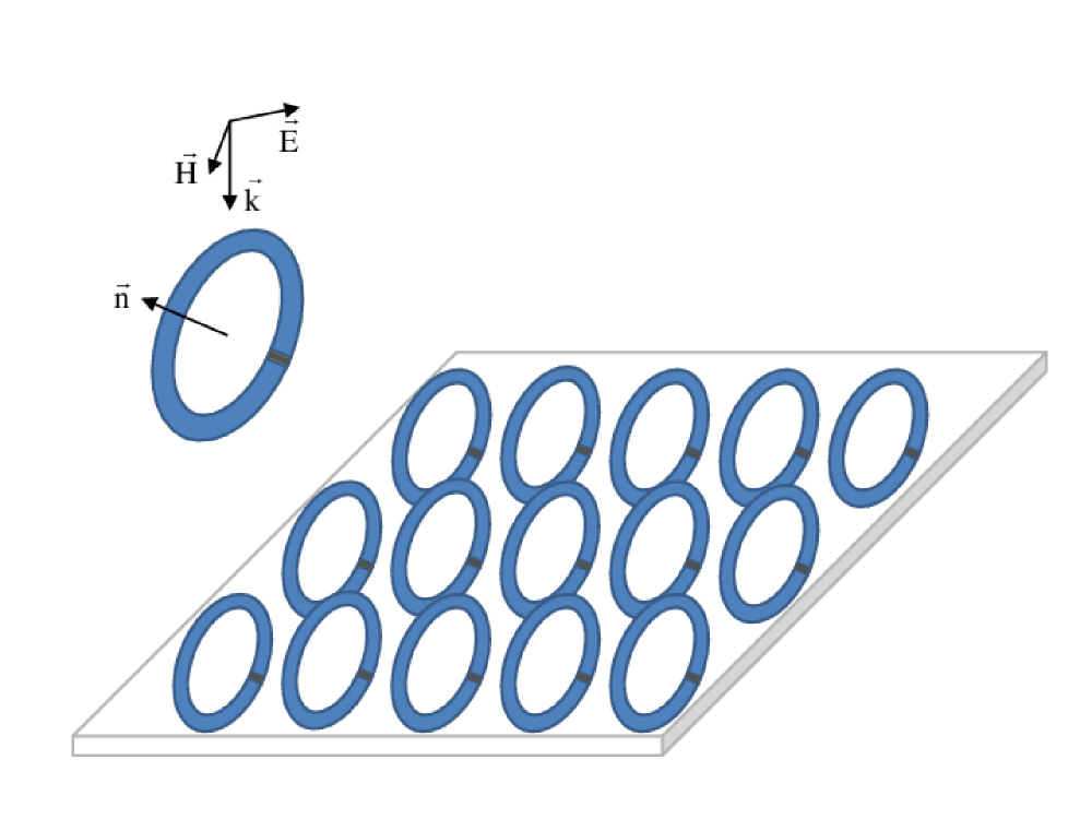
Figure 1: Schematic view of the electromagnetic wave incident on the layer containing split ring Josephson junction resonators. One ring is shown, indicating the orientation.

From Maxwell’s equations (1-3) we obtain the wave equation

$$\mathbf{H}_{tt}-{c^{2}\over\varepsilon}\Delta\mathbf{H}=-{1\over\mu_{0}}\mathbf{M}_{tt}.$$ (5)

Since the model considered is translationally invariant with respect to the $x$ axis, this equation can be presented as

$$\mathbf{H}_{tt}-{c^{2}\over\varepsilon}\mathbf{H}_{zz}=-{1\over\mu_{0}}\mathbf{M}_{tt}.$$ (6)

Let us now consider the Josephson split-ring part. The magnetic moment is

$$\mathbf{m}(t)=SI\mathbf{n},$$ (7)

where $I$ is the current in the loop (11). Combining the two equations (4) and (7) we get the final expression for $\mathbf{M}$

$$\mathbf{M}=SIn_{r}l\delta(z)\mathbf{n}.$$ (8)

Plugging the above expression into the wave equation (6) yields the wave equation

$$\mathbf{H}_{tt}-{c^{2}\over\varepsilon}\mathbf{H}_{zz}=-{1\over\mu_{0}}SI_{tt}n_{r}l\delta(z)\mathbf{n}.$$ (9)

As in cgm12 the current in the ring is given by

$$I=-L^{-1}(\Phi+2\pi\Phi_{0}\varphi),$$ (10)

where $\Phi$ is the flux induced by the electromagnetic field, where $L$ is the inductance of the loop, where $\varphi$ is the supraconducting phase in the junction and where $\Phi_{0}={\hbar\over 2\pi}$ is the reduced flux quantum. The flux $\Phi$ across the ring of area $S$ is

$$\Phi=S\mathbf{H}\cdot\mathbf{n}$$

where $\mathbf{n}$ is the normal vector to the ring. This gives us the current in the ring

$$I=-L^{-1}\left(S\mathbf{H}\cdot\mathbf{n}+2\pi\Phi_{0}\varphi\right).$$ (11)

The evolution of the variable $\varphi$ is the same as in cgm12 except that the current on the right hand side is modified. We have

$$2\pi C\Phi_{0}\frac{\partial^{2}\varphi}{\partial t^{2}}+2\pi{\Phi_{0}\over R}\frac{\partial\varphi}{\partial t}+I_{c}\sin\varphi=I.$$ (12)

Plugging (11) into (12) and multiplying by $L/(2\pi\Phi_{0})$ we get

$$LC\varphi_{tt}+{L\over R}\varphi_{t}+{LI_{c}\over 2\pi\Phi_{0}}\sin\varphi=-{S\over 2\pi\Phi_{0}}\mathbf{H}\cdot\mathbf{n}-\varphi.$$ (13)

Our model consists in the wave equation (9) together with the split-ring Josephson equation (13). These can be normalized as in cgm12 . The natural units of time, flux and space are

$$\omega_{T}=1/\sqrt{LC},~{}~{}\Phi_{0},~{}~{}z_{0}={c\over\omega_{T}\sqrt{\varepsilon}},$$

where $\omega_{T}$ is the Thompson frequency and $z_{0}$ is the inverse of the Thompson wave number. The magnetic field $\mathbf{H}$ is normalized as

$$\mathbf{h}={\mathbf{H}S\over 2\pi\Phi_{0}},~{}~{}\qquad\tau=\omega_{T}t,\qquad\zeta=z/z_{0}.$$ (14)

In terms of these variables the final equations are

$$\mathbf{h}_{\tau\tau}-\mathbf{h}_{\zeta\zeta}=\kappa\left(\mathbf{h}_{\tau\tau}\cdot\mathbf{n}+\varphi_{\tau\tau}\right)\delta(\zeta)\mathbf{n}.$$ (15)

$$\varphi_{\tau\tau}+\alpha\varphi_{\tau}+\varphi+\beta\sin\varphi=-\mathbf{h}\cdot\mathbf{n},$$ (16)

where the parameters $\alpha,~{}~{}\beta$ and $\kappa$ are

$$\alpha={1\over R}\sqrt{L\over C},~{}~{}\beta={LI_{c}\over 2\pi\Phi_{0}},~{}~{}\kappa={n_{r}lS^{2}\over\mu_{0}Lz_{0}}.$$ (17)

The equations (15,16) are our principal model and we now proceed to analyze them.

III Microwave spectroscopy data

As in cgm12 we assume that the film is submitted to a stationary field that will fix the phase $\varphi_{s}$. We can then write

$$\mathbf{h}=\mathbf{h}_{s}+\delta\mathbf{h},~{}~{}\varphi=\varphi_{s}+\delta\varphi$$

where the field $\delta\mathbf{h}$ and the variable $\delta\varphi$ are small. Their evolution is given by

$$\delta\mathbf{h}_{\tau\tau}-\delta\mathbf{h}_{\zeta\zeta}=\kappa\left(\delta\mathbf{h}_{\tau\tau}\cdot\mathbf{n}+\delta\varphi_{\tau\tau}\right)\delta(\zeta)\mathbf{n}.$$ (18)

$$\delta\varphi_{,\tau\tau}+\alpha\delta\varphi_{,\tau}+\delta\varphi+\beta\cos\varphi_{s}\delta\varphi=-\delta\mathbf{h}\cdot\mathbf{n}.$$ (19)

To solve the equations (18,19) we assume the usual harmonic dependence

$$\delta\mathbf{h}=e^{i\omega t}\mathbf{f},~{}~{}\delta\varphi=e^{i\omega t}\phi.$$

This yields the following equations

$$\mathbf{f}_{\zeta\zeta}+\omega^{2}\mathbf{f}=\omega^{2}\kappa\left(\mathbf{f}\cdot\mathbf{n}+\phi\right)\delta(\zeta)\mathbf{n},$$ (20)

$$\phi\left(\omega_{r}^{2}-\omega^{2}+\alpha i\omega\right)=-\mathbf{f}\cdot\mathbf{n},$$ (21)

where we have introduced the resonant frequency $\omega_{r}$

$$\omega_{r}^{2}=1+\beta\cos\varphi_{s}.$$ (22)

We now set up the scattering experiment by assuming an incident field and calculating the reflected and transmitted fields. For $\zeta<0$ we have

$$\mathbf{f_{-}}(\zeta)=\mathbf{f}_{\rm in}e^{-i\omega\zeta}+\mathbf{f}_{\rm r}e^{i\omega\zeta}.$$ (23)

For $\zeta>0$ the field is

$$\mathbf{f_{+}}(\zeta)=\mathbf{f}_{\rm tr}e^{i\omega\zeta}.$$ (24)

At the interface $\zeta=0$ $\mathbf{f}$ is continuous so that

$$\mathbf{f}_{\rm in}+\mathbf{f}_{\rm r}=\mathbf{f}_{\rm tr}.$$ (25)

We have the following jump condition for $\mathbf{f}_{\zeta}$

$$\left[\mathbf{f}_{\zeta}\right]_{0_{-}}^{0_{+}}=\kappa\omega^{2}(\mathbf{f}_{\rm tr}\cdot\mathbf{n}+\phi)\mathbf{n}.$$ (26)

This yields

$$\mathbf{f_{in}}-\mathbf{f_{r}}=\mathbf{f}_{\rm tr}-i\omega\kappa(\mathbf{f}_{\rm tr}\cdot\mathbf{n}+\phi)\mathbf{n}.$$ (27)

From the equations (25, 27) it follows

$$\mathbf{f_{in}}=\mathbf{f}_{\rm tr}-i\frac{\omega\kappa}{2}\mathcal{M}(\omega)](\mathbf{f}_{\rm tr}\cdot\mathbf{n})\mathbf{n},$$ (28)

$$\mathbf{f_{r}}=i\frac{\omega\kappa}{2}\mathcal{M}(\omega)(\mathbf{f}_{\rm tr}\cdot\mathbf{n})\mathbf{n},$$ (29)

where

$$\mathcal{M}(\omega)=1+(\omega^{2}-\omega_{r}^{2}-i\alpha\omega)^{-1}.$$ (30)

From the first equation we obtain

$$(\mathbf{f}_{\rm tr}\cdot\mathbf{n})=D(\omega)(\mathbf{f}_{\rm in}\cdot\mathbf{n}),$$ (31)

where

$$D(\omega)=\left[1-i\frac{\omega\kappa}{2}\mathcal{M}(\omega))\right]^{-1}.$$ (32)

Using these expressions we obtain

$$\mathbf{f_{r}}=i\frac{\omega\kappa}{2}\mathcal{M}(\omega)D(\omega)(\mathbf{f}_{\rm in}\cdot\mathbf{n})\mathbf{n},$$ (33)

$$\mathbf{f_{tr}}=\mathbf{f}_{\rm in}+i\frac{\omega\kappa}{2}\mathcal{M}(\omega)D(\omega)(\mathbf{f}_{\rm in}\cdot\mathbf{n})\mathbf{n}.$$ (34)

Equation (33) implies that the polarization of the reflected wave is determined by $\mathbf{n}$ only. On the other hand the direction of the transmitted wave depends on the orientations of $\mathbf{n}$ and $\mathbf{f}_{\rm in}$ and on the frequency $\omega$.

From expression (33) the reflection coefficient is

$$\mathcal{R}=\frac{|\mathbf{f_{r}}|^{2}}{|\mathbf{f_{in}}|^{2}}=\frac{(\omega\kappa/2)^{2}|\mathcal{M}(\omega)|^{2}\cos^{2}\theta}{1+(\omega\kappa/2)^{2}|\mathcal{M}(\omega)|^{2}},$$ (35)

where $\theta$ is defined by the formula

$$\mathbf{f}_{\rm in}\cdot\mathbf{n}=|\mathbf{f}_{\rm in}|\cos\theta.$$ (36)

The transmission coefficient is $\mathcal{T}=|\mathbf{f_{tr}}|^{2}/|\mathbf{f_{in}}|^{2}$. It is

$$\mathcal{T} = 1-\frac{(\omega\kappa/2)^{2}|\mathcal{M}(\omega)|^{2}\cos^{2}\theta}{1+(\omega\kappa/2)^{2}|\mathcal{M}(\omega)|^{2}}\cos^{2}\theta+$$

$$~{}~{}+i\frac{\omega\kappa}{2}\frac{[\mathcal{M}(\omega)-\mathcal{M}^{*}(\omega)]}{1+(\omega\kappa/2)^{2}|\mathcal{M}(\omega)|^{2}}\cos^{2}\theta=$$

$$= 1-\mathcal{R}-\frac{\omega\kappa~{}\mathrm{Im}\mathcal{M}(\omega)}{1+(\omega\kappa/2)^{2}|\mathcal{M}(\omega)|^{2}}\cos^{2}\theta.$$ (37)

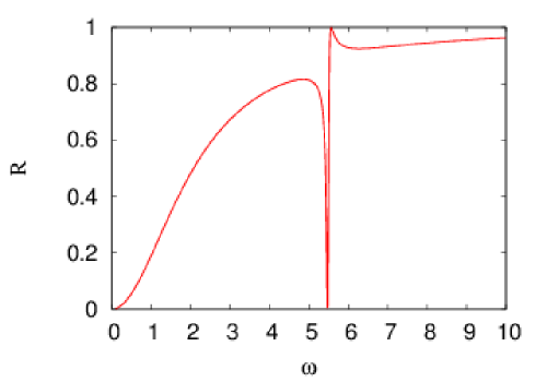
Figure 2: The reflection coefficient $\mathcal{R}(\omega)$ from (35) for a plane wave normally incident to the film,$\theta=0$.

Let us analyze numerically the reflection and transmission coefficients. We choose $\beta=30$ so that we are in the highly hysteretical case as in cgm12 . Fig. 2 shows the dependance of the reflection coefficient on $\omega$ for a normal incidence in the lossless case $\alpha=0$, when $\kappa=1$ and $\beta=30$. The external magnetic field $h_{s}$ is assumed to be zero. Then we can take $\varphi_{s}=0$ which is the global minima of the potential of the equation (16)(see Fig 2. in cgm12 ). The reflection coefficient shows a strong resonance for frequencies near $\omega_{r}$; this resonance is of the Fano type (see MFK:10 ). The value of the resonance frequency is

$$\omega_{r}=\sqrt{1+\beta\cos\phi_{s}}\approx 5.56.$$

The metasurface is transparent for small $\omega$; when the frequency is large the incident field is totally reflected. The shape of the spectrum does not depend on the specific value of $\beta$ and $\omega_{r}$. For instance, the experimentalists Ustinov:13 chose a smaller $\beta$ and obtain a reflection coefficient that behaves similarly to the one shown in Fig. 2.

The magnetic component of the reflected wave is always oriented in the direction of the normal. On the contrary, the polarization angle of the transmitted wave $\mathbf{f_{tr}}$ depends on the frequency $\omega$ and on the orientation of the split-ring (angle $\theta$). To analyze this dependance assume that the incident field is parallel to the $y$ axis.

$$\mathbf{f}_{\rm in}=\left(\begin{matrix}0\cr 1\cr 0\end{matrix}\right).$$

Then the reflected and transmitted fields can be written as

$$\mathbf{f}_{\rm r}=\left(\begin{matrix}0\cr R_{1}\cr R_{2}\end{matrix}\right),~{}~{}\mathbf{f}_{\rm tr}=\left(\begin{matrix}0\cr T_{1}\cr T_{2}\end{matrix}\right).$$

From the relations (30),(32),(33),(34) we get

$$R_{1}=T_{1}-1,~{}~{}R_{2}=T_{2},$$ (38)

$$T_{1}=D(\omega)\left[1-i{\kappa\omega\over 2}\sin^{2}\theta\mathcal{M}(\omega)\right],$$

$$T_{2}=-{i\kappa\omega\sin\theta\cos\theta\over 2}D(\omega)\mathcal{M}(\omega).$$ (39)

The transmission coefficient $\mathcal{T}(\omega)$ is shown in Fig. 3 for three different values of the orientation angle $\theta=2\pi/5,~{}~{}\pi/4$ and $\pi/6$.

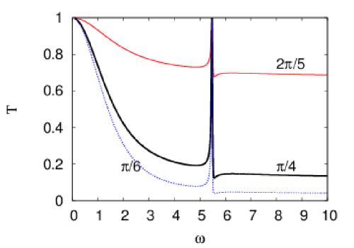
Figure 3: The transmission coefficient $\mathcal{T}(\omega)$ from (37) for a plane wave and three values of the orientation angle $\theta$ .

Note that the array is transparent $\mathcal{T}=1$ when $\omega=\omega_{r}$. Past this frequency, the transmission coefficient asymptotically tends to a constant. For a large angle $\theta=2\pi/5$, the ring has less influence, since most of the field is transmitted. When the angle is reduced, the incoming magnetic field interacts strongly with the rf-SQUIDs so the reflected field is stronger.

From the expression (39) for $T_{1,2}$ one obtains the angle of polarization rotation of the transmitted wave $\psi$ in the $(y,z)$ plane:

$$\psi=\arctan\left(\frac{\mathrm{Re}~{}T_{2}}{\mathrm{Re}~{}T_{1}}\right).$$ (40)

Fig. 4 shows this angle $\psi$ as a function of $\omega$ and $\theta$.

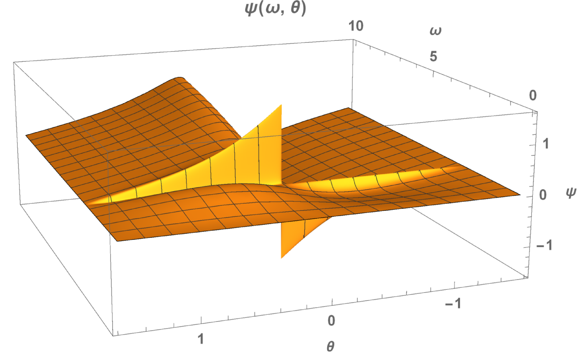
Figure 4: Angle $\psi(\omega)$ from (40) as function of $\omega$ and $\theta$, $\alpha=0$

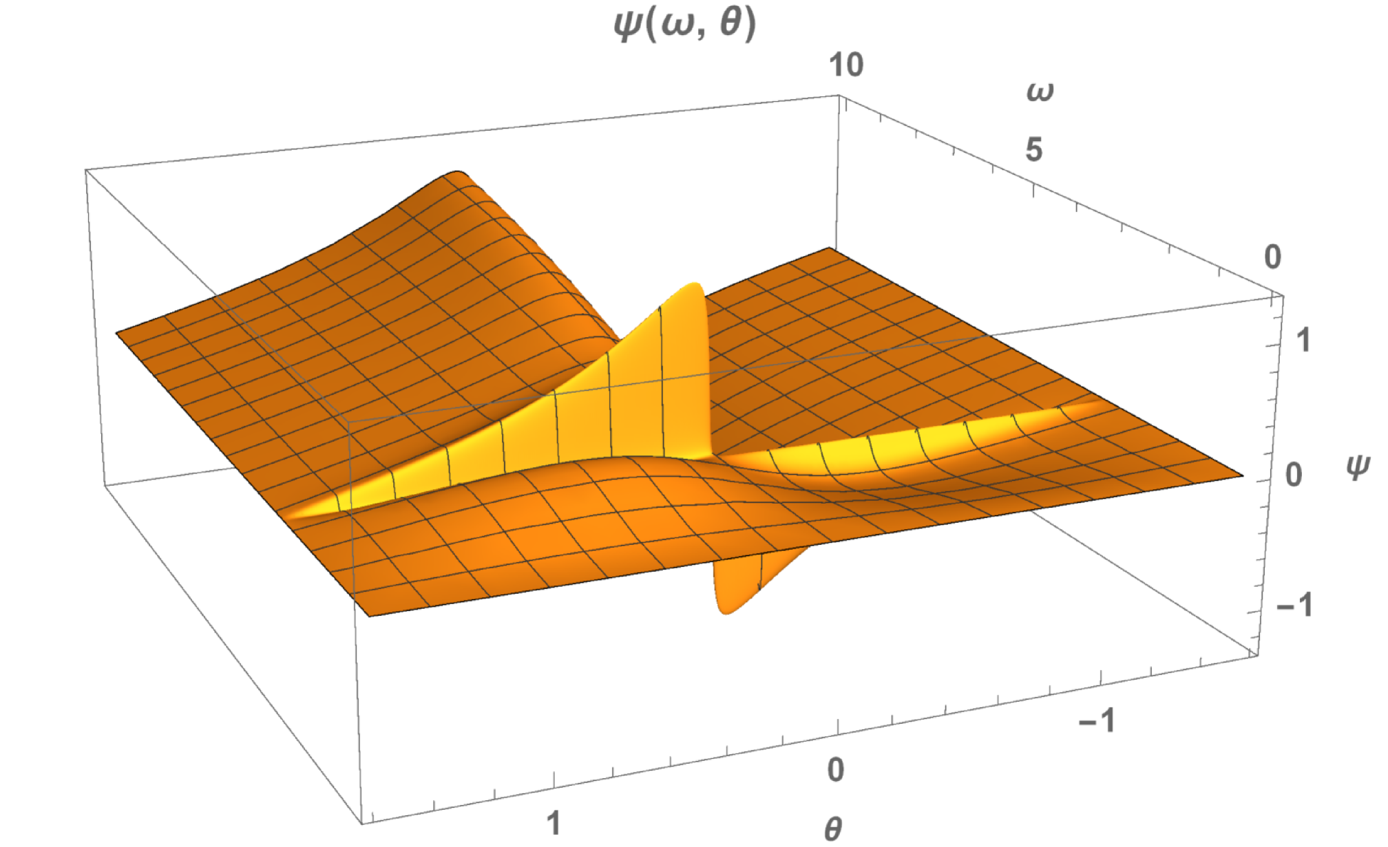
Figure 5: Angle $\psi(\omega)$ from (40) as function of $\omega$ and $\theta$, $\alpha=0.05$

Fig. 4 demonstrates the Faraday effect which takes place in rf-SQUID metasurface under consideration. The polarization rotation angle $\psi$ depends both on the frequency $\omega$ and on the inclination angle of the rf-SQUIDs. The angle of rotation of the polarization changes sharply near the resonant frequency $\omega_{r}$ (gigantic Faraday effect). This angle depends strongly on $\theta$; it has a pronounced resonance character near $\omega_{r}$. In this case, when $\theta$ changes from $-\pi/2$ to $0$ angle $\psi$ monotonically decrease from $0$ to $-\pi/2$. For $\theta=0$ the angle $\psi$ jumps from $-\pi/2$ to $\pi/2$ and monotonically decreases to $0$ when $\theta$ changes from $0$ to $\pi/2$ (see Fig.  4). Introducing losses which are always present in any practical situation smoothes the jump transition, Fig. 5.

IV Detailed study of the resonance

We study here the characteristics of the resonance of the coupled system – rf-SQUID and field. From equations (19) and (34) we can write the time dependent phase equation as (Maim:Gabi:10 )

$$\ddot{\varphi}(t)+\alpha\dot{\varphi}(t)+(1+\beta\cos\phi_{s})\varphi(t)=-f(t),$$ (41)

$$f(t)={\kappa\over 2}\left(\dot{\varphi}(t)+\dot{f}(t)\right)+k\cos\omega t.$$

Recalling the resonant frequency $\omega_{r}$ from (22) we replace

$$\cos\omega t\mapsto\exp(i\omega t).$$

so that the system (41) can be rewritten: The solutions of the resulting system have the following form:

$$\varphi(t)=A\exp(i\omega t),~{}~{}f(t)=B\exp(i\omega t),$$

$$A=-kC^{-1},~{}~{}B=k\left[(\omega_{r}^{2}-\omega^{2})+i\alpha\omega\right]C^{-1},$$

$$C=\omega_{r}^{2}-\omega^{2}(1-{\kappa\over 2}\alpha)+i\omega\left[\alpha+{\kappa\over 2}(1+\omega^{2}-\omega_{r}^{2})\right].$$

Representing $A$ in terms of a phase and an amplitude $A=a\exp(i\theta)$ we obtain:

$$a=\frac{k}{\sqrt{\left[\omega_{r}^{2}-\omega^{2}(1-(\kappa\alpha/2))\right]^{2}+\omega^{2}\left[\alpha+(\kappa/2)(1+\omega^{2}-\omega_{r}^{2})\right]^{2}}},$$

$$\tan\theta=\frac{\omega\left[\alpha+(\kappa/2)(1+\omega^{2}-\omega_{r}^{2})\right]}{\omega^{2}(1-(\kappa\alpha/2)-\omega_{r}^{2}}.$$

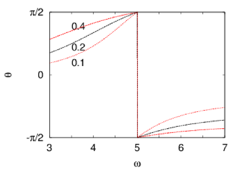
Figure 6: Plot of the amplitude $a(\omega)$ (left panel) and the phase $\theta(\omega)$ (right panel) for three different values of the coupling $\kappa=0.4,0.2$ and $0.1$. The other parameters are $\omega_{r}=5,\alpha=0.01$.

The amplitude $a$ and the phase $\theta$ are plotted as a function of the frequency $\omega$. Notice how the resonance gets sharper for a small coupling $\kappa$. We also have the typical jump in the phase as one crosses the resonance.

The amplitude $a(\omega)$ reaches its maximal value for

$$\omega_{max}^{2}=\frac{1}{3{\tilde{\kappa}}^{2}}\left[{\tilde{\kappa}}^{2}(2\omega_{r}^{2}-\alpha^{2}-2)-1\right]+$$

$$+\frac{1}{3{\tilde{\kappa}}^{2}}\bigg{[}1+{\tilde{\kappa}}^{2}\left[4+2\omega^{2}_{r}-\alpha^{2}-6{\tilde{\kappa}}\alpha+\right.$$

$$\left.{\tilde{\kappa}}^{2}\left[(\omega^{2}_{r}-1)\left[(\omega^{2}_{r}-1)-4\alpha^{2}\right]+\alpha^{4}\right]\right]\bigg{]}^{1/2}$$ (42)

where $\tilde{\kappa}=\kappa/2$. Since $\alpha$ and ${\tilde{\kappa}}$ are small, $\omega_{max}^{2}$ up to second order has following form:

$$\omega_{max}^{2}\approx\omega_{r}^{2}-\frac{\alpha^{2}}{2}-\alpha{\tilde{\kappa}}-\left(\omega_{r}^{2}+\frac{1}{2}\right){\tilde{\kappa}}^{2}$$

When $\omega$ is close to $\omega_{r}$, ($\omega=\omega_{r}+\Delta$, $|\Delta|\ll 0$) and $\alpha$ and ${\kappa}$ are small, then

$$a\approx\frac{k}{\omega_{r}\sqrt{4\Delta^{2}+(\alpha+{\tilde{\kappa}})^{2}}}$$ (43)

If ${\kappa}=0$, we recover the classical resonance observed for a damped driven linear oscillator, both for $\theta$ and $a$, landau .

V Conclusion

We analyzed the interaction of a plane electromagnetic wave with a two dimensional array of rf-SQUIDs. The wave vector of the incident field is assumed orthogonal to the array of rf-SQUIDs. All rf-SQUIDs have the same inclination with respect to the surface of the array and the effective thickness of this ”array film” is much smaller then the wavelength. Our main result is that despite this small thickness, the array effectively controls the wave reflection and transmission. In particular, it changes the polarization of the reflected wave and this change is determined only by the orientation of the rf-SQUIDs. This effect is identical to the Kerr effect in a gyrotropic medium. Here the gyrotropy is introduced by the rf-SQUIDs. The polarization of the transmitted wave also changes and depends both on the carrier frequency and on the inclination angle of the rf-SQUIDs. This is similar to a Faraday effect. At the resonance frequency we obtain a gigantic Faraday effect. We emphasize that the thickness of the array is always much smaller than the wave-length.

This array of rf-SQUIDs acts as a meta-surface that controls the polarization of an electromagnetic wave. The analysis that we carried out is limited by the linear approximation. Increasing the incident field will cause a larger current in the ring and subsequently a nonlinear response of the rf-SQUIDs. We then expect nonlinear Kerr and Faraday effects combined with bistability.

VI Acknowledgement

The research of A.I.M. was supported by Russian Scientists Found (project 14-22-00098). The research of I.R.G. was partially supported by the Ministry of Education and Science of Russian Federation (Project DOI: RFMEFI58114X0006). J. G. C. thanks the Region Haute-Normandie for support through a research grant GRR-LMN and the CRIHAN computing center for the use of its facilities.

References

- (1) N. Yu et al, ”Light propagation with phase discontinuities: generalized laws of reflection and refraction”, Science, 334, 333-337, (2011).
- (2) X. Ni et al , ”Broadband light bending with plasmonic nanoantennas”, Science, 335, 427, (2012).
- (3) N. Lazarides, G. P. Tsironis, and M. Eleftheriou, ”Dissipative discrete breathers in rf SQUID metamaterials”, arXiv:0712.0719v1 [nlin.PS] 2007
- (4) N. Lazarides, and G. P. Tsironis, ”rf superconducting quantum interference device metamaterials”, Appl. Phys. Lett. 90, 163501 (2007).
- (5) G. P. Tsironis, N. Lazarides, and M. Eleftheriou, ”Dissipative Breathers in rf SQUID Matamaterials” PIERS Proc. March 23-27, China, Beijin 2009 p. 52-56 (2009).
- (6) A.I. Maimistov, I. Gabitov, Nonlinear response of a thin metamaterial film containing Josephson junctions, Opt.Commun. 283, 1633-1639 (2010).
- (7) Chunguang Du, Hongyi Chen, and Shiqun Li, ”Quantum left-handed metamaterial from superconducting quantum-interference devices”, Phys.Rev. B74, 113105 (2006).
- (8) St.M Anlage, ”The physics and applications of superconducting metamaterials”, J.Opt. 13, 024001 (2011).
- (9) M. Trepanier, Daimeng Zhang, O. Mukhanov, and St. M. Anlage, ”Realization and Modeling of Metamaterials Made of rf Superconducting Quantum-Interference Devices”, Phys.Rev. X 3, 041029 (2013).
- (10) J.-G. Caputo, I. Gabitov and A.I. Maimistov , ”Electrodynamics of a split-ring Josephson resonator in a microwave line”, Phys Rev. B 85, 205446 (2012).
- (11) A.E. Miroshnichenko, S. Flach, Y.S. Kivshar, Fano resonances in nanoscale structures, Reviews of Modern Physics 82 (3), 2257, (2010)
- (12) P. Jung, S. Butz, S. V. Shitov, and A. V. Ustinov, ”Low-loss tunable metamaterials using superconducting circuits with Josephson junctions”, Appl.Phys.Lett. 102, 62601 (2013).
- (13) N. Lazarides, G.P. Tsironis, and Yu.S. Kivshar ”Surface breathers in discrete magnetic metamaterials”, Phys.Rev. E 77, 065601(R) (4 pages) (2008).
- (14) M. Eleftheriou, N. Lazarides, G.P.Tsironis ”Magnetoinductive breathers in metamaterials”, Phys.Rev. E77, 036608 (13 pages) (2008).
- (15) M. Eleftheriou, N. Lazarides, G.P.Tsironis, and u.S. Kivshar ”Surface magnetoinductive breathers in two-dimensional magnetic metamaterials”, Phys.Rev. E80, 017601 (4 pages) (2009).
- (16) L. Landau and E. Lifchitz, ”Cours de physique théorique”, Mecanique Mir, Moscou.