De-Confinement and Clustering of Color Sources in Nuclear Collisions

Abstract

A brief introduction of the relationship of string percolation to the
Quantum Chromo Dynamics (QCD) phase diagram is presented. The behavior of the Polyakov loop close to the critical temperature is studied in terms of the color fields inside the clusters of overlapping strings, which are produced in high energy hadronic collisions. The non-Abelian nature of the color fields implies an enhancement of the transverse momentum and a suppression of the multiplicities relative to the non overlapping case. The prediction of this framework are compared with experimental results from the SPS, RHIC and LHC for $pp$ and AA collisions. Rapidity distributions, probability distributions of transverse momentum and multiplicities, Bose-Einstein correlations, elliptic flow and ridge structures are used to evaluate these comparison.

The thermodynamical quantities, the temperature, and energy density derived from RHIC and LHC data and Color String Percolation Model (CSPM) are used to obtain the shear viscosity to entropy density ratio ($\eta/s$). It was observed that the inverse of ($\eta/s$) represents the trace anomaly $\Delta=(\varepsilon-3P)/T^{4}$. Thus the percolation approach within CSPM can be successfully used to describe the initial stages in high energy heavy ion collisions in the soft region in high energy heavy ion collisions. The thermodynamical quantities, temperature and the equation of state are in agreement with the lattice QCD calculations. Thus the clustering of color sources has a clear physical basis although it cannot be deduced directly from QCD.

1 Introduction

1.1 Motivation and historical perspective

Before the discovery of the quarks there was an interest in the behavior of matter at high density and/or high temperature [1]. This interest was increased with the formulation of QCD and the possibility of distributing high energy or high nucleon density over a large volume to temporary restore broken symmetries of the physical vacuum creating abnormal dense states of nuclear matter [2].

Very early after QCD was born, it was pointed out that the asymptotic freedom property of QCD implies the existence of a high density matter formed by deconfined quarks and gluons [3] and the exponential increasing of the spectrum of Hagedorn was connected to the existence of a different phase, in which quarks and gluons are deconfined [4]. The thermalized phase of quarks and gluons was called Quark Gluon Plasma (QGP) [5] and it was realized that the required high density could be achieved in relativistic heavy-ion collisions [6, 7] and several signatures of QGP were proposed. Quarkonium suppression [8], anomalous excess of photons and jet quenching [9, 10] were some of them. At this time, it was pointed out the relevance of percolation in the study of the phase structure of hadronic matter [11, 12].

Experimentally there was a large effort to study in laboratory the deconfinement and chiral symmetry restoration phase transitions and to explore the properties of high density matter starting by the AGS and ISR experiments and continued at SPS, RHIC and LHC. The SPS accelerator experiments already displayed several signatures that hinted at the onset of QGP formation [13]. The RHIC data show a striking bulk collective elliptic flow, which is generated at relatively early times, since otherwise the spatial anisotropy could not convert into a momentum spatial anisotropy. The flow pattern was consistent with a very low shear viscosity over entropy density ratio $\eta/s$, indicating strongly interacting matter. On the other hand, jet quenching phenomena were clearly observed indicating that this deconfined strongly interacting matter was very opaque [14, 15, 16, 17, 18]. The above mentioned ratio gave rise to an increasing interest on the AdS/CFT correspondence due to the result $\eta/s=1/4\pi$ [19].

The recent LHC experiments [20, 21, 22] have extended the study of the elliptic flow to all the harmonics [23, 24] confirming that the high quark gluon density matter interacts strongly. The collective behavior and the ridge structure observed previously at RHIC in Au-Au and Cu-Cu collisions [25, 26], was also observed in pPb [27, 28, 29] and pp interactions [30] at high multiplicity at the LHC. The collective flow of pPb and the ridge structure of pPb and pp collisions is a challenge to the usual hydrodynamic descriptions. On the other hand, the data on quarkonium seems each time to confirm more the validity of the combined picture of a sequential melting of the different resonances together with recombination of heavy quarks and antiquarks at high energy [31, 32, 33]. Also a detailed study of the jet quenching for identified particles has been performed [34] showing interesting features related to the loss of coherence of the gluons emitted in the jet due to the high density medium.

From the theoretical side in addition to the hydrodynamic studies the Color Glass Condensate(CGC) picture [35, 36, 37, 38, 39] derived directly from QCD, is very appealing and gives a reasonable description of most of the experimental observables. At first sight, due to the non-Abelian nature of QCD, with gluons carrying color charge, the gluon density $xG(x,Q)$ rises rapidly as a function of the decreasing fractional momentum $x$, or increasing the resolution $Q_{s}$. So, the gluon showers generate more gluon showers producing an exponential avalanche toward small $x$. As the transverse size of the hadron or the nucleus rises slowly at high energies, the number of gluons and their density per unit of area and rapidity increase rapidly as $x$ decreases. However, there will be fusion of gluons leading to a limited transverse density of gluons at some fixed momentum resolution $Q_{s}$ and that is gluon saturation [40]. The low $x$ gluons are closely packed, the distance between them being very small, hence the interaction coupling is weak $\alpha_{s}\ll$ 1. Weak couplings systems are adequate to be studied in QCD. In a given collision the multiplicity should be proportional to the number of gluons, which at the saturation momentum $Q_{s}$, is [41, 42].

$$\frac{dN}{dy}\sim\frac{1}{\alpha_{s}(Q_{s})}Q_{s}^{2}R^{2}.$$ (1)

This dense system, called CGC, has a very high occupation number $1/\alpha_{s}(Q_{s})$ and corresponds to a highly coherent state of strong color fields. The high $x$ gluons can be regarded as the sources of the low $x$ gluons. The independence on the cutoff, used to separate the high $x$ gluons from the low $x$ ones, gives rise to a kind of evolution equation. In the infinite momentum frame, these large momentum gluons travel very fast and therefore their time scales are Lorentz dilated.

Due to the Lorentz contraction the collision of two nuclei can be seen as that of two sheets of colored glass where the color field in each point of the sheets is randomly directed. Taking these fields as initial conditions, one finds that between the sheets longitudinal color electric and magnetic fields are formed. The number of these color flux tubes between the two colliding nuclei is $Q_{s}^{2}R^{2}$ forming Glasma [43], which has been extensively applied to compare with experimental data.

An alternative approach to the CGC is the percolation of strings [44, 45, 46, 47, 48] subject of this report. The percolation of strings is not directly obtained from QCD and only is QCD inspired. In string percolation, multiparticle production is described in terms of color strings stretched between the partons of the projectile and target. These strings decay into $q-\bar{q}$ and $qq-\bar{qq}$ pairs and subsequently hadronize producing the observed hadrons. Due to the confinement, the color of these strings is confined to a small area $S_{1}=\pi r_{0}^{2}$, with $r_{0}$=0.2 fm in the transverse space. With increasing energy and/or size and centrality of the colliding objects, the number of strings grows and the strings start to overlap forming clusters, very similar to discs in 2-dimensional percolation theory [49]. At a given critical density, a macroscopic cluster appears crossing the collision surface, which marks the percolation phase transition. Therefore the nature of this transition is geometrical.

In string percolation the basic ingredients are the strings, and it is necessary to know their number, rapidity extension, fragmentation and number distribution. All that requires a model and therefore string percolation is model dependent. However most of the QCD inspired models give very similar results for most of the observables in such a way that the predictions are by a large measure independent of the model used.

The string percolation and the Glasma are related to each other [50]. In the limit of high density there is a correspondence between physical quantities of both approaches. The number of color flux tubes in the Glasma picture, $Q_{s}^{2}R^{2}$, has the same dependence on the energy and on the centrality of the collision that the number of effective clusters of strings in string percolation. In both approaches for the multiplicity distribution a negative binomial distribution is obtained, where the parameter ${\it k}$ that controls the width has the same energy and centrality dependence. The role of the occupation number $1/\alpha_{s}$ in CGC is played by the fraction of the total available surface covered by the strings formed in the collision. The randomness of the color field in the CGC gives rise to a reduction of the expected multiplicity. Similarly the randomness of the direction in color space of the color field of the ${\it{n}}$ strings of the cluster stipulates that the strength of the resulting field is not ${\it{n}}$ times the strength of the individual color field but $\sqrt{n}$. This reduction also implies a reduction of the multiplicity of particles produced in the collision. Due to all these similarities in both approaches the predictions for different physical observables are very similar. The string percolation is able to explore also the region where the limit of high density has not been reached.

The plan of the review is as follows: After this introduction in the two next chapters the phase structure of QCD and the main results of lattice QCD are briefly studied. Percolation studies related to QCD are briefly reviewed and later the color string percolation model is introduced. In the following sections the applications of the model to the description of transverse momentum distributions, rapidity and multiplicity distributions, azimuthal distributions, harmonic momenta and ridge structures, Bose-Einstein correlations, $J/\Psi$ suppression, and forward-backward correlations are described. Finally, the thermodynamics in the production of particles in string percolation is studied starting by relating the critical percolation density with the critical temperature. Afterwards we study the equation of state, the behavior of the trace anomaly and ratio between the shear viscosity and the entropy density with temperature.

1.2 Phase diagram of nuclear matter

What is the behavior of matter when we increase its density? The observed densities of our world expand over many orders of magnitude, from $\sim 10^{-6}$ nucleons/$cm^{3}$ in average in the Universe to $\sim 10^{38}$ nucleons/$cm^{3}$ inside a nucleus and $\sim 10^{39}$ nucleons/$cm^{3}$ in a neutron star. The study of the high density limit, specifically the confinement transition from hadrons to quarks and gluons can be regarded as the place where the high energy collision (two body) probes the short distance limit and therefore meets the thermodynamics (many body) of this short distance dynamics [51].

Let us start by studying the behavior of a high density medium under electromagnetic forces. In a high density medium, the Coulomb potential between two electric charges

$$V(r)\approx\frac{e^{2}}{r}$$ (2)

becomes screened in such a way that the new potential

$$V(r)\approx\frac{e^{2}}{r}\exp(-r/r_{0}(\rho))$$ (3)

disappears for $r>r_{0}$, where $r_{0}$ is the Debye screening radius, which decreases as the charge density $\rho$ increases. This potential change occurs because other charges in the medium are around the two original ones, reducing the interaction. In this way the interaction range becomes shorter. If we consider a bound electromagnetic state, like a hydrogen atom and increase the density the Debye radius eventually becomes smaller than the binding radius of the atom $r_{0}<r$ and the force between the proton and electron is reduced so that the two particles can no longer be bound. An insulator material consisting of bound electrical charges at high density becomes a conductor, it undergoes a phase transition, the Mott transition [52]. The charge screening dissolves the binding of the constituents giving rise to a new state of the matter, the plasma. In this transition, the electrons change their mass from the usual physical mass in the insulator phase to an effective medium electron mass. In fact, the electrons in the conducting phase move in the periodic field of the ions, which is very different from the vacuum. In the case of QCD, we have confinement, which means that the lines of the color field between two color charges are no longer expanded into all the space like in the case of Coulomb potential between electrical charges but are confined to a rather small space region, forming hadrons, which are colorless bound states of colored quarks.

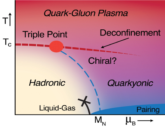
Figure 1: Phase diagram of the nuclear matter. Temperature vs baryonic chemical potential [53].

However, at high color charge density we expect that color screening takes place resulting in an exponential damping of the potential and removing all the long range effects of the confining potential. In this way, we expect that color screening transforms a color insulator into a color conductor, leading to deconfinement of quarks from hadrons [54]. This transition, like the insulator to conductor in the electromagnetic case, is a collective effect, in which many charges participate, and we expect a behavior like a phase transition.

In a similar way to the electron mass, the quark masses are expected to change between the two phases. In the confined phase the quarks are dressed with gluons, acquiring an effective constituent mass of around 300 MeV (1/3 of the proton mass). For light quarks this constituent mass is much larger than their mass appearing in the QCD Lagrangian where it is close to zero. In another words, the light quark mass in the confined phase is generated by the confinement interaction, and when deconfinement occurs this additional mass disappears.

The role of gluons would be to generate the effective quark mass, maintaining spontaneous chiral symmetry breaking. There will be need of a higher temperature $T$ or baryonic potential $\mu$ to evaporate or melt the gluonic density of quarks leading to deconfined quarks and gluons with restored chiral symmetry. According to this picture, from the hadronic phase, first it is the dressed quark phase [55] and after the deconfined and the restoration of chiral symmetry. In this picture, there are two scales: First, the hadronic scale $R_{h}=$ 1 fm when the density $\rho$ is below

$$\rho_{h}\sim\frac{1}{(4/3)\pi R_{h}^{3}}.$$ (4)

and the medium is of hadronic nature. For densities $\rho$

$$\rho_{h}<\rho<\rho_{q}\sim\frac{1}{(4/3)\pi R_{q}^{3}}$$ (5)

with $R_{q}\sim 0.3$ fm the medium consists of deconfined massive quarks. Finally, for densities $\rho>\rho_{q}$ the medium becomes quarks and gluons phase with restoration of chiral symmetry.

This picture could be true if the scale $R_{q}$ were independent of $T$ and $\mu$. However, the lattice studies have shown, that near $\mu=0$, color deconfinement and chiral symmetry restoration coincide. Hence, in a medium of low baryon density, the mass of the constituent quark vanishes at the deconfinement point $T_{c}$ and also the screening radius of the gluon cloud size vanishes. At low $T$ and high $\mu$, there is no reason to expect a similar behavior and probably there will be an intermediate region of massive dressed quarks between the hadronic phase and the deconfined and chiral symmetry restoration phase. At low $T$ and high $\mu$, other possibilities could exist as quarkyonic matter and color superconductivity [56, 57, 58]. A possible phase diagram is shown in Fig. 1 [53].

1.3 Lattice QCD

In finite temperature lattice QCD, the deconfinement order parameter is provided by the vacuum expectation value of the Polyakov loop $L(\vec{x})$ defined in Euclidean space

$$L(\vec{x})={\rm Tr}\prod_{t=1}^{N_{t}}A_{4}(\vec{x},t)$$ (6)

$L(\vec{x})$ is the ordered product of the SU(3) temporal gauge variables $A_{4}(\vec{x},t)$ at a fixed spatial position, where $N_{t}$, is the number of lattice points in time direction and Tr denotes the trace over color indices. The Polyakov loop corresponds to a static quark source and its vacuum expectation value is related to the free energy $F_{q}$ of a single quark

$$L(\vec{x})\sim\exp\Big{(}-\frac{F_{q}}{T}\Big{)}.$$ (7)

Below the critical temperature $T_{c}$ quarks are confined and $F_{q}$ is infinite implying $\langle L(\vec{x})\rangle$=0. In a deconfined medium color screening among the gluons makes $F_{q}$ finite, hence for $T>T_{c}$ $\langle L(\vec{x})\rangle\neq 0$. The breaking of chiral symmetry is controlled by the chiral condensate $X(T)\equiv\langle\bar{\Psi}\Psi\rangle\sim M_{q}$ which measures the constituent quark masses obtained from a Lagrangian with massless quarks. At high temperature this mass melts, therefore

$$X(T)_{=0\,T>T_{x}}^{\neq 0\,T<T_{x}}.$$ (8)

$T_{x}$ defines another critical temperature. The corresponding derivatives with respect to $T$ of $\langle L\rangle$ and $X$, the susceptibilities, have been studied in finite temperature lattice QCD at vanishing baryon number, showing a sharp peak that defines respectively $T_{c}$ and $T_{x}$. The two temperatures, within errors, coincide. Also seen is a sharp transition, i.e. a crossover. The quoted value of $T_{c}$ is 155 $\pm 9$ MeV [59, 60, 61].

Energy densities resulting from lattice QCD are shown in Fig. 2(left) indicating that even for $T>3T_{c}$ its values are far from the energy density of a free gas of quarks and gluons, namely

$$\varepsilon=\frac{\pi^{2}}{30}[g_{g}+\frac{7}{8}(q_{q}+q_{\bar{q}})]T^{4}.$$ (9)

where $g_{g}$, $g_{q}$ and $g_{\bar{q}}$ are the degeneracy numbers of the gluons, quarks and antiquarks. This fact indicates that in a rather broad range of temperatures the deconfined phase is a strongly interacting medium. This is better seen looking at the interaction measure

$$\Delta=(\varepsilon-3P)/T^{4}.$$ (10)

The energy momentum tensor trace

$$T_{\mu}^{\mu}=\frac{B(g_{s})}{2g_{s}}G_{\mu\nu}^{a}G^{\mu\nu a}+[1+r(g_{s})]m_{q}\bar{\Psi}_{q}\psi_{q}$$ (11)

is ($\varepsilon-3P$) and even for massless quarks $T_{\mu}^{\mu}\neq 0$ as a consequence of the introduction of the scale in the re-normalization process breaking the conformal symmetry (trace anomaly). In Fig. 2 (right) the results of lattice QCD are shown. $\Delta$ decreases with ${\it T}$ very slowly, even less than $1/T^{2}$. The deconfined medium interacts strongly for a broad range of temperatures above ${\it T}$.

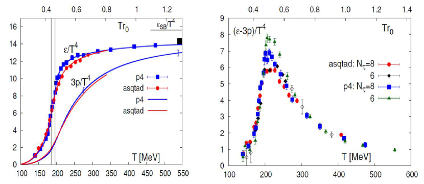
Figure 2: The energy density and the pressure as function of temperature (left). The energy density shows a sharp rise in the temperature region 170-200 MeV. The interaction measure calculated using different staggered fermion actions (right) [61].

1.4 Percolation

A simple example of percolation is the 2-dimensional continuous percolation, which will be used extensively studying string percolation [49, 62]. Let us distribute small discs of area $\pi r_{0}^{2}$ randomly on a large surface, allowing overlap between them. As the number of discs increases clusters of overlapping discs start to form. If we regard the discs as small drops of water, how many drops are needed to form a puddle crossing the considered surface? Given $N$ discs, the disc density is $\rho=N/S$ where $S$ is the surface area. The average cluster size increases with $\rho$, and at a certain critical value $\rho_{c}$ the cluster spans the whole surface as shown in Fig. 3 [51] .

The critical density for the onset of continuum percolation has been determined by numerical and Monte-Carlo simulations for different systems, which in 2- dimensional case gives

$$\rho_{c}=\frac{1.13}{\pi r_{0}^{2}}.$$ (12)

In the thermodynamical limit corresponding to $N\rightarrow\infty$, keeping $\rho$ fixed, the distribution of overlaps of the discs is Poissonian with a mean value $\xi=\rho\pi r_{0}^{2}$, $\xi$ being a dimensionless quantity

$$P_{n}=\frac{\xi^{n}}{n!}\exp(-\xi).$$ (13)

Hence the fraction of the total area covered by discs is $1-\exp(-\xi)$ [47].

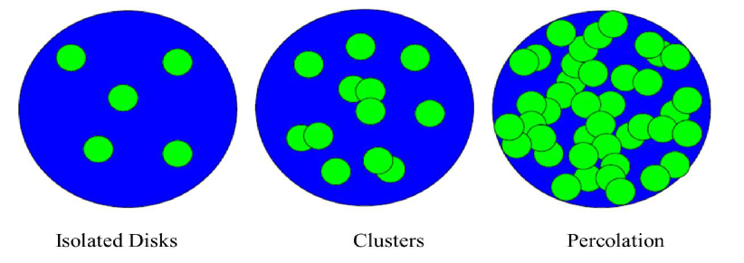
Figure 3: Left panel: Disconnected discs, Middle: Cluster formation, Right panel: Overlapping discs forming a cluster of communication [51].

For the critical value of 1.13 around 2/3 of the area is covered by discs. This number 1.13 is obtained for the case of an homogeneous surface [62, 49]. In cases of non homogeneous surface profiles, this factor changes. For example, in the cases of circular surfaces with Gaussian or Wood-Saxon profiles the critical percolation is reached at

$$\rho_{c}=\frac{1.5}{\pi r_{0}^{2}}.$$ (14)

Also the fraction of the area covered by strings is no longer given by $1-\exp(-\xi)$, but by the function [63]

$$\frac{1}{1+a\exp(-(\xi-\xi_{c})/b)}$$ (15)

where $\xi_{c}$ =1.5. The parameters $a$ and $b$ depend on the profile function. In particular $b$ controls the ratio between the width of the border of the profile (2$\pi R$) and the total area ($\pi R^{2}$), therefore is proportional to $1/R$.

Three-dimensional percolation has been applied to study the phase boundaries of high density matter. As mentioned earlier, even before the discovery of the quarks, Pomeranchuk [1] realized that above a certain high density hadrons lost their identity. In fact, when the density of a gas of hadrons is increased by raising either the temperature or the baryon density, a quark of a given hadron will be closer to some quark or antiquark of other hadrons than to the original partners. The identity of hadronic matter is lost and now there is deconfined quark and antiquark matter. At $\mu=0$, the percolating density for mesons and low density baryons is

$$\rho_{c}\simeq\frac{1.24}{(4/3)\pi R_{h}^{3}}\simeq 0.6fm^{-3},$$ (16)

where $R_{h}$= 0.8 fm is the hadron radius. This is the density of the percolating cluster at the onset of perco1ation. If we place overlapping spheres in a large volume, the critical density for the percolating spheres is [49, 63, 64]

$$\rho_{c}\simeq\frac{0.34}{(4/3)\pi R_{h}^{3}}\simeq 0.16fm^{-3}.$$ (17)

However at this point only 29$\%$ of the space is covered by the overlapping spheres and 71$\%$ remain empty, very different from that in 2-dimensional percolation. Here, both spheres and empty space form infinite connected networks or clusters. The density given by Eq. (17) gives the normal nuclear matter density. The more accurate critical percolation density for the onset of the deconfinement transition is given by Eq. (16), leading to a density 4 times larger than nuclear matter. The existence of two percolation thresholds, one for the formation of a spanning cluster of spheres and another for the disappearance of a spanning vacuum cluster is a general feature of percolation in three or more dimensions.

Assuming that for the density of 0.6-0.8 $fm^{-3}$ the cluster is formed by an ideal gas of all hadrons and resonances, the temperature of such a gas at this density is 170-190 MeV [65] which is not far from the critical temperature obtained in lattice QCD of $\sim$ 155 MeV. The critical density Eq. (17) implies that the average distance between quark and antiquark at the deconfined point is $d_{q}\simeq 1/\rho_{c}^{1/3}\simeq$ 1.2 fm.

At high $\mu$ and $T$ = 0 one should consider percolation of nucleons having an impenetrable spherical hard core, of radius R around $R_{h}/2$. Each sphere defines a volume $V=\frac{4/3}{\pi R_{h}^{3}}$, which is not accessible to the center of any other sphere. The spheres can only overlap partially and the distance between their centers must be larger than $R=2R$. Then we have again two percolation thresholds. Numerical studies show that in the case of the spheres forming a spanning cluster there is no variation in the value of the critical density, however for the case of the vacuum percolation threshold, now we have [65]

$$\rho=\frac{2}{(4/3)\pi R_{h}^{3}}\simeq 0.93fm^{-3}.$$ (18)

The disappearance of the vacuum cluster for hard spheres requires a higher density than needed for permeable spheres. At this point, it is interesting to explore the percolation of constituents of mass $M_{q}\sim$ 300 MeV and radius $R_{q}\sim$ 0.3 fm. In this case the critical density will be

$$\rho=\frac{1.2}{(4/3)\pi R_{q}^{3}}\simeq 3.5fm^{-3}.$$ (19)

This value is 4 times larger than the critical value for nucleon percolation (0.93 $fm^{-3}$) and 22 times the normal nuclear matter density (0.16 $fm^{-3}$). According to this, massive deconfined quarks exist between the hadronic matter and the deconfined quarks and gluons state. In this intermediate state the quarks are deconfined, but the gluons are bound into the constituents quarks. In the lower baryon density limit, the quarks bind into nucleons. In the higher baryon density limit a connected medium of deconfined quarks and gluons is obtained. Also at fixed baryon density and increasing $T$ the deconfined quarks and gluons and the restoration of the chiral symmetry is found.

Let us mention that in the SU(3) lattice gauge theory, spatial clusters can be identified as those where the local Polyakov loops $\langle L(\vec{x})\rangle$ have values close to some element of the center. The elements of the center group $Z_{3}$, are a set of three phases $[0,2\pi/3,-2\pi/3]$ [66]. Below $T_{c}$, ($\langle L(\vec{x})\rangle=0$) the values of $\langle L(\vec{x})\rangle$ grouped around these three phases, show three pronounced peaks located at the center phases. Above $T_{c}$, $\langle L(\vec{x})\rangle\neq 0$ the distribution changes. One of the peaks grows and the other two shrink. A spontaneous symmetry breaking occurs, which leads to a non vanishing $\langle L(\vec{x})\rangle$. Spatial clusters can be defined grouping the sites with a very similar value of $\langle L(\vec{x})\rangle$. The weight of the largest cluster increases sharply at $T=T_{c}$ as seen in Fig. 4. Also the diameter of the largest cluster, that remains constant below $T_{c}$, starts to rise quickly at $T=T_{c}$ being 40 times larger at $T=1.2T_{c}$ indicating that the cluster percolates. These results do not change using ensembles with different lattice spacing. Therefore in the pure gauge SU(3) theory the deconfinement transition is a percolation phase transition (of the second order).

In the case of full QCD [67], the fermions break the center symmetry explicitly and act as an external magnetic field in the Ising model, which favors the phase 0 of the Polyakov loop, although the other two phases ($\pm 2\pi/3)$ remain populated. As in the pure gauge case at $T=T_{c}$ there is a pronounced increase of the dominant phase. The explicit breaking of the center symmetry leads to a crossover type of transition. This suggests that the chiral symmetry restoration phase transition also can be related to a generalized percolation phase transition [68]. These properties of the Polyakov loop, giving rise to domain like structure or clusters of deconfined matter could explain its large opacity as well as its near ideal fluid properties, being the origin of the elliptic flow [69].

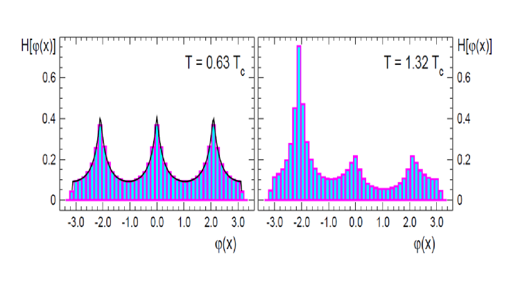
Figure 4: Histograms for the distributions of the phase $\phi(x)$ of the local loops $\langle L(\vec{x})\rangle$. The left plot shows the distribution below $T_{c}$ while distribution in deconfined phase is shown in the right plot [66].

In experimental collisions at high energy, we expect that color strings are formed between the projectile and target partons. These color field configurations must have a small transverse size due to confinement. In this way, the strings are seen as small discs in the total available surface of the collisions. As the number of strings grows with energy and centrality degree of the collision, these strings would overlap forming clusters which eventually percolate. This 2-dimensional percolation and its phenomenological consequences in relation to SPS, RHIC and LHC pp, pA and AA data is the main subject of this review. In this case the critical percolation density is given by Eq. (12) or Eq. (14) in case of realistic profiles.

1.5 String models

The phenomenology of string percolation takes its main ingredient, the strings, from models, even though most of the predictions are not dependent on the details of the models. Majority of the models roughly coincide in basic postulates such as the number of strings and its dependence on energy and centrality, which is taken from the Glauber-Gribov model. Strings models can be divided in models with color exchange between projectile and target as the Dual Parton Model (DPM) [70, 71, 72], Quark Gluon String Model (QGSM) [73], VENUS [72], EPOS [74], DPMJET [75] and models without color exchange where the interaction excites the projectile and target producing strings between the partons of both. Examples of this kind of models are HIJING [76], PYTHIA [77], AMPT [78], HSP [79], and URQMD [79]. We will concentrate in models with color exchange, essentially the DPM, which are based on the $1/N_{c}$ QCD expansion and are in correspondence via unitarity with the Gribov Reggeon calculus. The DPM or QGSM have been extensively compared to the experimental data of ISR, SPS and FermiLab obtaining an overall agreement [70].

In DPM or QGSM, the multiplicity distribution dN/dy of pp collisions is described by the formation and fragmentation of ${\it 2k}$ strings [70] as shown in Fig. 5(a).

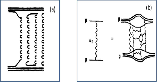
Figure 5: (a):Two cut Pomeron diagram (four chain) for proton-proton collisions. (b):Single Pomeron exchange and its underlying cylindrical topology. This is a dominant contribution to proton-proton elastic scattering at high energies [70].

$$\frac{dN^{pp}}{dy}=\frac{1}{\sigma}\sum{\sigma_{k}[N_{k}^{qq-q}(s,y)+N_{k}^{q-qq}(s,y)+(2k-2)N_{k}^{q-\bar{q}}(s,y)]},$$ (20)

where $N_{k}^{q-qq}$ and $N_{k}^{q-qq}$ are the inclusive spectra of hadrons produced in the strings stretched between a valence diquark of the projectile (target) and a quark of the target (projectile) and $N_{k}^{q-\bar{q}}$ are the inclusive spectra of the strings stretched between sea quarks and antiquarks. The single particle distribution of each string can be obtained by folding the momentum distribution of the partons at the end of the string with the fragmentation function of the string

$$N_{1}^{qq-q}(s,y)=\int_{0}^{1}\int_{0}^{1}dx_{1}dx_{2}\rho_{k}(x_{1})\rho_{k}(x_{2})\frac{dN^{qq-q}}{dy}(y-\bar{\Delta},s_{s}),$$ (21)

Here $\sqrt{s_{s}}$ is the invariant mass of the string, $s_{s}=sx_{1}x_{2}$, where $x_{1}$ and $x_{2}$ are the light-cone momentum fractions of the constituents at the ends of the string. $\bar{\Delta}$ is the rapidity shift necessary to go from the overall pp center of mass (CM) frame to the CM of one string,

$$\bar{\Delta}=\frac{1}{2}\log(\frac{x_{1}}{x_{2}})$$ (22)

The momentum distributions used for the valence quarks, sea quarks or antiquarks and valence diquarks are $x^{-1/2}$, $x^{-1}$, and $x^{3/2}$ respectively. In general, the distribution of 2$k$ partons in the proton is

$$\rho_{k}(x_{1},x_{2k};x_{2},x_{3},....x_{2k-1})=C_{k}^{\rho}x_{1}^{-1/2}x_{2}^{-1}...x_{2k-1}^{-1}x_{2k}^{3/2}\delta(1-\sum_{1}^{2k}x_{i}),$$ (23)

where $C_{k}^{\rho}$ can be found by normalizing $\rho_{k}$ to unity.

With these momentum distributions the $N^{qq-q}$ and $N^{q-qq}$ strings are long (due to $x^{3/2}$ and $x^{-1/2}$ behavior of their extremes) centered at a rapidity point shifted with respect to the CM. The $N^{q-q}$ strings are short, centered at the CM (due to the $x^{-1}$ of their constituents ends). Concerning the fragmentation functions different methods have been used even within the same model. In string percolation, mostly the Schwinger mechanism or the Lund fragmentation is used. In Eq. (20) $\sigma_{k}$ is the cross section for producing 2$k$ strings resulting from cutting $k$ Pomerons.

As the Pomeron has the topology of a cylinder its cutting gives rise to two strings (Fig. 5(b)). Using the AGK cutting rules [80], the dependence of $\sigma_{k}$ with the energy is given by

$$\sigma_{k}=\frac{8\pi g\exp(\Delta y)}{kz}[1-e^{-z}\sum_{l=0}^{k-1}\frac{z^{l}}{l!}],\ \ k>0,$$ (24)

where

$$z=\frac{2gC\exp(\Delta y)}{R^{2}+\alpha^{{}^{\prime}}y}$$

and $g$ is the coupling of the Pomeron to the proton, 1+$\Delta$ the intercept of the trajectory of the Pomeron, $\alpha^{{}^{\prime}}$ its slope and $\mathcal{C}$ a parameter describing the inelastic diffractive states ($\mathcal{C}=$1 means only elastic scattering without diffractive states). The total cross section is obtained summing over $k$

$$\sigma_{tot}=\exp(\Delta y)\sum_{k=0}^{\infty}\sum_{l=k,l>0}^{\infty}(\frac{-z}{2})^{l-1}\frac{8\pi g}{l!}[\delta_{k0}+(-1)^{1-k}2^{l-1}(^{l}_{k})].$$ (25)

The rise of dN/dy is mainly due to short strings, whose number grows with energy. On the other hand, outside the region of central rapidity there is no contribution of these short strings and the rise with energy is much slower. Assuming a Poisson distribution for cutting $k$ Pomerons

$$P_{k}(n)=\frac{(kN)^{n}}{n!}\exp(-kN),$$ (26)

where $N$ is the mean multiplicity produced when cutting one Pomeron, the multiplicity distribution is

$$P_{k}(n)=\sum_{k}w_{k}P_{k}(n),\ \ w_{k}=\frac{\sigma_{k}}{\sigma}.$$ (27)

Very often $<n>P(n)$ is plotted as a function of $n/<n>$. When the result is independent of energy one has the well-known Koba-Nielsen-Olesen (KNO) scaling. KNO scaling is roughly obeyed up to the highest ISR energy ($\sqrt{s}$ = 63 GeV) but it is clearly violated at SPS, Fermilab, RHIC and LHC. The origin of KNO violation can be understood in DPM easily. The contributions of multistrings diagrams become increasingly important when ${\it s}$ increases, and since they contribute mostly to high multiplicities they push upwards the high multiplicity tail. The increase with $s$ of the multistrings contributions is due both to the increase of the invariant mass of short strings and to the ${\it s}$-dependence of the weights. Hence, we expect a larger KNO violation at central rapidity region where the short strings contribute than in the whole rapidity range or close to the ends of the phase space where the short strings do not contribute.

The width of the KNO multiplicity distributions is related to the fluctuations of the number of strings, which also control the forward-backward correlations. These correlations can be described by the approximate linear expression

$$<n_{b}>=a+bn_{f},$$ (28)

where $n_{f(b)}$ is the number of particles observed in the forward (backward) rapidity window and $a$ and $b$ are given by

$$a=\frac{<n_{b}><n_{f}>^{2}-<n_{f}n_{b}><n_{f}>}{<n_{f}^{2}>-<n_{f}>^{2}},$$

$$b=\frac{<n_{f}n_{b}>-<n_{f}><n_{b}>}{<n_{f}^{2}>-<n_{f}>^{2}}.$$ (29)

Usually the forward and backward rapidity intervals are taken separated by a central rapidity window $|y|<y_{c}$ in such a way that the short range correlations are eliminated ($y_{c}>$ 0.5). Consider symmetric forward and backward intervals, $\delta y_{F}=\delta y_{B}=\delta y$. In any multiple scattering model the origin of long range correlations is the fluctuations in the number of multiple scatterings [81, 82, 83]. Let $N$ strings decay each into $\mu$ particles on the average. The slope $b$ can be split into short range correlations (SR) and long range correlations (LR) [84]

$$b=b_{SR}+b_{LR}=\frac{\beta}{1+C}+\frac{C}{1+C},$$ (30)

where $\beta$ is the ratio between the forward-backward variance and the forward-forward variance of the distribution of particles produced in a single string:

$$\beta=\frac{D_{FB}}{D_{FF}}=\frac{<\mu_{f}\mu_{b}>-<\mu_{f}><\mu_{b}>}{<\mu_{f}^{2}>-<\mu_{f}>^{2}}$$ (31)

and

$$C=\frac{D_{N}\mu_{F}^{2}}{<N>D_{FF}},\ \ D_{N}=<N^{2}>-<N>^{2}.$$ (32)

For a large rapidity window between the forward and backward intervals, there are no long range correlations in a single string, $D_{FB}$ = 0 and we have

$$b=\frac{1}{1+\frac{<N>D_{FF}}{D_{N}\mu_{F}^{2}}}.$$ (33)

Usually it is assumed that the multiplicity distribution of a single string is Poissonian, $D_{FF}=\mu_{F}$ and $b$ becomes

$$b=\frac{1}{1+\frac{<N>}{D_{N}\mu_{F}}}.$$ (34)

According to Eq. (34), at low energy there are no fluctuations in the number of strings, $D_{N}$ = 0 and ${\it b}$ = 0. As the energy increases, $D_{N}$ increases as well as $b$. On the other hand, if we fix the multiplicity we eliminate many of the string fluctuations and therefore $b$ is smaller.

The generalization of DPM to nucleus-nucleus collisions is obtained as follows [85]. Consider a collision of a nucleus A with nucleus B in a configuration with $N_{A}$ participating nucleons of A, $N_{B}$ participating nucleons of B (assume that $N_{A}\leq N_{B}$) and a total number $N_{c}$ of inelastic collisions. In this configuration hadrons are produced in 2$N_{c}$ strings (2 strings for each inelastic collision). Of these 2$N_{A}$ are stretched between valence quarks and valence diquarks ($q_{v}^{A}-qq_{v}^{B}$ and $qq_{v}^{A}-q_{v}^{B})$. The remaining $N_{B}-N_{A}$ valence quarks and diquarks of B have no valence partner of A and have to form $2N_{B}-2N_{A}$ strings with sea quarks and antiquarks of A ($q_{s}^{A}-qq_{v}^{B}$ and $\bar{q}_{s}^{A}-q_{v}^{B}$). The remaining $2N_{c}-2N_{B}$ strings are formed between sea quarks and antiquarks of A and B ($q_{s}-\bar{q}_{s}$)

$$\frac{dN^{AB}}{dy}=\frac{1}{\sigma_{AB}}\sum_{N_{A},N_{B},N_{c}}[\sigma_{N_{A},N_{B},N_{c}}^{AB}\theta(N_{B}-N_{A})N_{A}(N^{qq_{v}^{A}-q_{v}^{B}}(y)+N^{q_{v}^{A}-qq_{v}^{B}}(y))+$$

$$(N_{B}-N_{A})(N^{\bar{q}_{s}^{A}-q_{s}^{B}}(y)+N^{q_{s}^{A}-qq_{v}^{B}}(y))+$$

$$(N_{c}-N_{B})(N^{q_{s}^{A}-\bar{q}_{s}^{B}}(y)+N^{\bar{q_{s}}^{A}-q_{s}^{B}}(y))+sym(N_{A}\leftrightarrow N_{B})],$$ (35)

where $\sigma_{N_{A},N_{B},N_{C}}^{AB}$ is the cross section for $N_{C}$ inelastic nucleon-nucleon collisions involving $N_{A}$ nucleons of A and $N_{B}$ nucleons of B. This cross section have been studied extensively [86, 87, 88] together with its different approximations needed for its evaluation. The inclusive spectra, as in the pp case, are given by a convolution of momentum distribution and fragmentation functions. In the case of A=B we have approximately

$$\frac{dN^{AA}}{dy}\approx<N_{A}>(2N^{qq-q_{v}}(y)+(2<k>-2)N^{q_{s}-\bar{q}_{s}}(y))+$$

$$(<N_{c}>-<N_{A}>)2<k>N^{q_{s}-\bar{q}_{s}}(y),$$ (36)

where we have introduced the possibility of having $k$ multiple scattering in the individual nucleon-nucleon interactions, which was neglected in the Eq. (35). Notice that in the term proportional to the number of collisions it is not specified if the collision is soft or hard. In fact there are many inelastic soft collisions included in this term. Sometimes it is wrongly assumed that the term proportional to the number of collisions contains only hard collisions. We observe that in the central rapidity region we have $2Nk$ strings which for high energy and heavy nuclei is a very large number (more than 1500). Due to that we expect interaction among them, and therefore they will not fragment in an independent way. We study later such interactions.

In hadron-nucleus interactions in DPM, QGSM or VENUS the multiplicity distribution $P(n)$ can be approximated by a negative binomial distribution.

2 Color strings with fusion and percolation

2.1 Introduction

As indicated in Section 1.5, multiparticle production at high energies can be described in terms of color strings stretched between the projectile and target  [71, 72, 73, 89, 90, 91]. Hadronization of these strings produces the observed hadrons. The basic characteristic feature of the color string model with fusion and percolation, which is the subject of this review, is that strings are provided with a finite area in the transverse space. In terms of gluon color field they can be considered as the color flux tubes stretched between the colliding partons, which in the transverse space are restricted to a finite disc of a given radius, dictated by the confinement. The mechanism of particle creation is then similar to the one in the well-known Schwinger mechanism of pair creation in a constant electric field covering all the space, except that now the space is finite in the transverse plane. Note that pair creation actually splits the space filled with the chromoelectric field into two parts, each of them attached to one of the initial and one of the created partons. In this way the dynamics of the string evolution consists of successive breaking into more strings.

So creation of particles goes via emission of $q\bar{q}$ pairs in the field of the string. From the start it is relevant to mention one of the important properties of this mechanism. The transverse dimension of the string is a characteristic independent of the form of the distribution of created partons in the transverse momentum, in contrast to what one may think considering the string itself as a distribution of partons (say gluons). In the latter case the average transverse momentum of emitted particles is obviously inverse to the transverse dimension of the source. However it is apparently not so for the Schwinger mechanism. With the field constant in the transverse plane the spectrum of constituents (photons in the QED case) is just the $\delta$-function. However the emitted electrons have non-zero transverse momenta whose average is determined by the strength of the field (although the total transverse momentum of the pair is indeed zero). Likewise in our color string picture emitted partons have average transverse momenta determined by the strength of the chromoelectric field and do not depend on the transverse dimension of the string.

At low energies for collision of hadrons and nuclei with relatively small atomic numbers the fact that strings have finite dimension has no influence on the results. In the transverse plane strings are projected as discs at large distances from one another and particle creation does not feel their interaction. However with growing energy and/or atomic number of colliding particles, the number of strings grows. Once strings have a certain nonzero dimension in the transverse space they start to overlap forming clusters, very much like discs in the 2-dimensional percolation theory. The geometrical behavior of strings in the transverse plane then follows that of percolating discs. In particular at a certain critical string density a macroscopic cluster appears (infinite in the thermodynamic limit), which marks the percolation phase transition  [44, 45, 46].

The percolation theory governs the geometrical pattern of the string clustering. Its observable implications however require introduction of some dynamics to describe string interaction, that is, the behavior of a cluster formed by several overlapping strings.

One can study different possibilities.

A most naive attitude is to assume that nothing happens as strings overlap, in other words, they continue to emit particles independently without being affected by their overlapping neighbors. This is a scenario of non-interacting strings, which closely corresponds to original calculations in the color strings approach, oriented at comparatively small energies (and numbers of strings). This scenario however contradicts the idea that strings are areas of the transverse space filled with color field and thus with energy, since in the overlapping areas the energy should have grown.

In another limiting case one may assume that a cluster of several overlapping strings behaves as a single string with an appropriately higher color field (a string of higher color, or a “color rope”  [92]). This fusion scenario was proposed by the authors and later realized as a Monte-Carlo algorithm nearly decades ago  [93, 94, 95]. It predicts lowering of total multiplicities and forward-backward correlations (FBC) and also strange baryon enhancement, in a reasonable agreement with the known experimental trends.

However both discussed scenarios are obviously of a limiting sort. In a typical situation strings only partially overlap and there is no reason to expect them to fuse into a single stringy object, especially if the overlap is small. The transverse space occupied by a cluster of overlapping strings splits into a number of areas in which different number of strings overlap, including areas where no overlapping takes place. In each such area color fields coming from the overlapping strings will add together. As a result the total cluster area is split in domains with different color field strength. As a first approximation, neglecting the interaction at the domain frontiers, one may assume that emission of $q\bar{q}$ pairs in the domains proceeds independently, governed by the field strength (“the string tension”) in a given domain. This picture implies that clustering of strings actually leads to their proliferation, rather than fusion, since each particular overlap may be considered as a separate string. Evidently newly formed strings differ not only in their colors but also in their transverse areas. As a simple example consider a cluster of two partially overlapping strings (Fig. 6) [47].

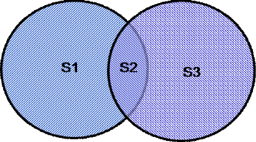
Figure 6: Projections of two overlapping strings onto the transverse plane [47].

One distinguishes three different regions: regions 1 and 3 where no overlapping takes place and the color field remains the same as in a single string, and the overlap region 2 with color fields of both strings summed. In our picture particle production will proceed independently from these three areas, that is, from three different “strings” corresponding to areas 1, 2 and 3. In this sense string interaction has split two strings into three of different color, area and form in the transverse space.

We stress that these dynamical assumptions are rather independent of the geometrical picture of clusterization. In particular, in each of the scenarios discussed above, at a certain string density there occurs the percolation phase transition. However its experimental signatures crucially depend on the dynamical contents of string interaction. With no interaction, clustering does not change physical observables, so that the geometric percolation will not be felt at all. With the interaction between strings turned on, clustering (and percolation) lead to well observable implications.

In this chapter we shall review these implications for the most immediate and important observables, multiplicities and transverse momenta spectra of produced particles.

2.2 Multiplicity and transverse momentum for overlapping strings

As stated in the Introduction, the central dynamical problem is to find how the observables change when several strings form a cluster partially overlapping. Let us consider a “simple” string stretched between a quark and antiquark with a transverse area $S_{1}$. It emits partons with the transverse momentum distribution

$$I_{0}(y,p)\equiv\frac{4\pi d\sigma}{dyd^{2}p}=Ce^{-\frac{m_{\perp}^{2}(p)}{t_{1}}}$$ (37)

where $t_{1}$ is the tension of the simple string, $m_{\perp}^{2}=m^{2}+p^{2}$ and $m$ and $p$ are the mass and transverse momentum of the emitted parton. In the following we mostly consider emitted pions when we take $m=0$. In accordance with the Schwinger picture of particle emission we assume that tension $t_{1}$ is proportional to the field responsible for emission and thus to the color charge at the string ends  [92, 96]. For the simple string stretched between the quark and antiquark it is proportional to the quark color charge squared $Q_{0}^{2}$. According to Eq. (37) the average transverse momentum squared is given by tension $t_{1}$: ${\Big{\langle}}p_{t}^{2}{\Big{\rangle}}_{1}=t_{1}$ and so is proportional to $Q_{0}$. We denote the multiplicity of produced particles per unit rapidity as $\mu_{1}$. It is also proportional to the color charge  [92, 96].

Now consider two simple strings, of areas $S_{1}$ in the transverse space each, partially overlap in the area $S^{(2)}$ (region 2 in Fig. 6), so that $S^{(1)}=S_{1}-S^{(2)}$ is the area in each string not overlapping with the other. A natural assumption seems to be that the average color density $q$ of the simple string in the transverse plane is a constant $q=Q_{0}/S_{1}$. For partially overlapping strings the color in each of the two non-overlapping areas will then be

$$Q_{1}=qS^{(1)}=Q_{0}(S^{(1)}/S_{1}).$$ (38)

In the overlap area each string will have color

$$\bar{Q}_{2}=qS^{(2)}=Q_{0}(S^{(2)}/S_{1}).$$ (39)

The total color in the overlap area $Q_{2}$ will be a vector sum of the two overlapping colors $qS_{2}$. In this summation the total color squared should be conserved  [92]. Thus $Q_{2}^{2}=({\bf Q}_{ov}+{\bf Q}^{\prime}_{ov})^{2}$ where ${\bf Q}_{ov}$ and ${\bf Q}^{\prime}_{ov}$ are the two vector colors in the overlap area. Since the colors in the two strings may generally be oriented in an arbitrary manner respective to one another, the average of ${\bf Q}_{ov}{\bf Q}^{\prime}_{ov}$ is zero. Then $Q_{2}^{2}=Q^{2}_{ov}+{Q^{\prime}_{ov}}^{2}$, which leads to

$$Q_{2}=\sqrt{2}\,qS^{(2)}=\sqrt{2}\,Q_{0}(S^{(2)}/S_{1}).$$ (40)

One observes that, due to its vector nature, the color in the overlap is less than the sum of the two overlapping colors. This phenomenon was first mentioned in  [92] for the so-called color ropes.

As mentioned, the simplest observables, the multiplicity $\mu$ and the average transverse momentum squared ${\Big{\langle}}p_{t}^{2}{\Big{\rangle}}$, are directly related to the field strength in the string and thus to its generating color. They are both proportional to the color [92, 96]. Thus, assuming independent emission from the three regions 1, 2, and 3 in Fig. 6 we get for the multiplicity

$$\mu/\mu_{1}=2(S^{(1)}/S_{1})+\sqrt{2}\,(S^{(2)}/S_{1}),$$ (41)

where $\mu_{1}$ is a multiplicity for a single string. To find ${\Big{\langle}}p_{t}^{2}{\Big{\rangle}}$ one has to divide the total transverse momentum squared of all observed particles by the total multiplicity. In this way for our cluster of two strings we obtain

$${\Big{\langle}}p_{t}^{2}{\Big{\rangle}}/{\Big{\langle}}p_{t}^{2}{\Big{\rangle}}_{1}=\frac{2(S^{(1)}/S_{1})+\sqrt{2}\sqrt{2}\,(S^{(2)}/S_{1})}{2(S^{(1)}/S_{1})+\sqrt{2}\,(S^{(2)}/S_{1})}$$

$$=\frac{2}{2(S^{(1)}/S_{1})+\sqrt{2}\ (S^{(2)}/S_{1})},$$ (42)

where ${\Big{\langle}}p_{t}^{2}{\Big{\rangle}}_{1}$ is the average transverse momentum squared for a simple string and we have used the evident property $2S^{(1)}+2S^{(2)}=2S_{1}$ in the second equality.

Generalizing to any number $N$ of overlapping strings we find the total multiplicity as

$$\mu/\mu_{1}=\sum_{i}\sqrt{n_{i}}\,(S^{(i)}/S_{1}),$$ (43)

where the sum goes over all individual overlaps $i$ of $n_{i}$ strings having areas $S^{(i)}$. Similarly for the ${\Big{\langle}}p_{t}^{2}{\Big{\rangle}}$ we obtain

$${\Big{\langle}}p_{t}^{2}{\Big{\rangle}}/{\Big{\langle}}p_{t}^{2}{\Big{\rangle}}_{1}=\frac{\sum_{i}n_{i}\,(S^{(i)}/S_{1})}{\sum_{i}\sqrt{n_{i}}\,(S^{(i)}/S_{1})}=\frac{N}{\sum_{i}\sqrt{n_{i}}\,(S^{(i)}/S_{1})}.$$ (44)

In the second equality we again used an evident identity $\sum_{i}n_{i}\,S^{(i)}=NS_{1}$. Note that Eqs. (43) and (44) imply a simple relation between the multiplicity and transverse momentum

$$\frac{\mu}{\mu_{1}}\frac{{\Big{\langle}}p_{t}^{2}{\Big{\rangle}}}{{\Big{\langle}}p_{t}^{2}{\Big{\rangle}}_{1}}=N,$$ (45)

which evidently has a meaning of conservation of the total transverse momentum produced.

Equations (43) and (44) do not look easy to apply. To calculate the sums over $i$ one seems to have to identify all individual overlaps of any number of strings with their areas. For a large number of strings the latter may have very complicated forms and their analysis presents great calculational difficulties. However one immediately recognizes that such individual tracking of overlaps is not at all necessary. One can combine all terms with a given number of overlapping strings $n_{i}=n$ into a single term, which sums all such overlaps into a total area of exactly $n$ overlapping strings $S^{tot}_{n}$. Then one finds instead of Eq. (43) and (44)

$$\mu/\mu_{1}=\sum_{n=1}^{N}\sqrt{n}\,(S^{tot}_{n}/S_{1})$$ (46)

and

$${\Big{\langle}}p_{t}^{2}{\Big{\rangle}}/{\Big{\langle}}p_{t}^{2}{\Big{\rangle}}_{1}=\frac{N}{\sum_{n=1}^{N}\sqrt{n}\,(S_{n}^{tot}/S_{1})}.$$ (47)

In contrast to individual overlap areas $S^{(i)}$ the total ones $S_{n}^{tot}$ can be easily calculated (see next subsection). Let the projections of the strings onto the transverse space be distributed uniformly in the total interaction area $S$ with a density $\rho$. Introduce a dimensionless parameter (“percolation parameter”)

$$\xi=\rho S_{1}=NS_{1}/S.$$ (48)

$\xi$: From Eq. (46) we then find that the multiplicity is damped due to overlapping by a factor

$$F(\xi)=\frac{\mu}{N\mu_{1}}=\frac{{\Big{\langle}}\sqrt{n}{\Big{\rangle}}}{\xi},$$ (49)

where the average is taken over the Poissonian distribution Eq. (13).

The behavior of $F(\xi)$ is shown in Fig. 7(a). It smoothly goes down from unity at $\xi=0$ to values around 0.5 at $\xi=4$ falling as $1/\sqrt{\xi}$ for larger $\xi$’s. According to Eq. (47) the inverse of $F$ shows the rise of the ${\Big{\langle}}p_{t}^{2}{\Big{\rangle}}$.

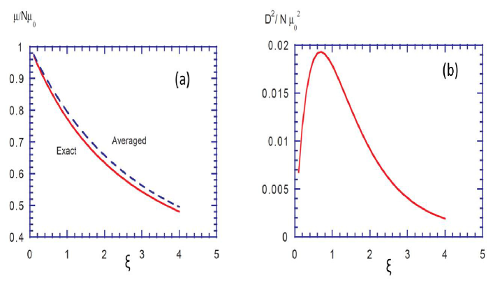
Figure 7: (a). Damping of the multiplicity as a function of $\xi$. (b): Percolation dispersion squared of the multiplicity per string in units $\mu_{1}^{2}$ as a function of $\xi$ [47].

Note that a crude estimate of $F(\xi)$ can be done from the overall compression of the string area due to overlapping. The fraction of the total area occupied by the strings according to Eq. (13) (see also  [97]) is given by

$$\sum_{n=1}{\cal P}_{n}=1-e^{-\xi}.$$ (50)

The compression is given by Eq. (50) divided by $\xi$. According to our picture the multiplicity is damped by the square root of the compression factor, so that the damping factor is

$$F(\xi)=\sqrt{\frac{1-e^{-\xi}}{\xi}}.$$ (51)

For all the seeming crudeness of this estimate, Eq. (51) is very close to the exact result, as shown in Fig. 7(a) by a dashed curve.

2.3 Multiplicities and their dispersion

In our picture in the transverse space simple strings are represented by discs of radius $r_{0}$ and area $S_{1}=\pi r_{0}^{2}$ homogeneously distributed in the total area $S$. We normalize $S$ assuming that centers of the discs are inside the unit circle of area $S_{0}=\pi$ so that $S=\pi(1+a)^{2}$, where $a$ is the normalized disc radius. The disc density is $\rho=N/S$ and the percolation parameter is $\xi=\rho S_{1}=NS_{1}/S$. In the thermodynamic limit $N\rightarrow\infty$, so that at fixed $\xi$ the radius of the discs goes to zero. For fixed $\xi$, $a^{2}=\xi/(\sqrt{N}-\sqrt{\xi})^{2}$, so that with our normalization at large $N$ $a\sim 1/\sqrt{N}$ and $S_{1}\sim 1/N$. Since the discs are distributed homogeneously, the probability that their centers are at points $r_{i}$, $i=1,...N$ inside the unit circle is independent of $r_{i}$ and is given by

$$P(r_{i})=1/S_{0}^{N}.$$ (52)

With the disc centers at points $r_{i}$. the overlap area of exactly $n$ discs is given by the integral

$$S_{n}^{tot}(r_{1},...r_{N})=\int_{S}d^{2}r\sum_{\{i_{1},..i_{n}\}\subset\{i_{1},...i_{N}\}}\prod_{k=1}^{n}\theta(a-|{\bf r}-{\bf r}_{i_{k}}|)\prod_{k=n+1}^{N}\theta(|{\bf r}-{\bf r}_{i_{k}}|-a).$$ (53)

The average of $S_{n}^{tot}$ will be given by a multiple integral over $r_{i}$ with the probability Eq. (52):

$${\Big{\langle}}S_{n}^{tot}{\Big{\rangle}}=\frac{1}{S_{0}^{N}}\int_{S_{0}}\prod_{i=1}^{N}d^{2}r_{i}S_{n}^{tot}(r_{1},...r_{N})=C_{N}^{n}\int_{S}d^{2}rF^{n}(r)(1-F(r))^{N-n},$$ (54)

where

$$F(r)=(1/S_{0})\int_{S_{0}}d^{2}r_{1}\theta(a-|{\bf r}-{\bf r}_{1}|).$$ (55)

The function $S_{0}F(r)$ gives an area occupied by a circle $C$ of radius $a$ with a center at $r$ which is inside the unit circle $S_{0}$. If $r<1-a$ then $C$ is always inside $S_{0}$ so that

$$F(r)=\sigma_{0}/S_{0},\ \ \ 0<r<1-a.$$ (56)

However for $r>1-a$ a part of $C$ turns out to be outside the unit circle, and

$$F(r)=\sigma(r)/S_{0},\ \ \ 1-a<r<1+a,$$ (57)

where $\sigma(r)\leq S_{1}$ is the overlap of the two discs $C$ and $S_{0}$.

Generally, the overlap of two circles of radii $r_{1}$ and $r_{2}$ with a distance $r$ between their centers is given by

$$\sigma(r_{1},r_{2},r)=(1/2)r_{1}^{2}(\alpha_{1}-\sin\alpha_{1})+(1/2)r_{2}^{2}(\alpha_{2}-\sin\alpha_{2}),$$ (58)

where

$$\cos(\alpha_{1}/2)=\frac{1}{2r_{1}}\left(r+\frac{r_{1}^{2}-r_{2}^{2}}{r}\right),$$

$$\cos(\alpha_{2}/2)=\frac{1}{2r_{2}}\left(r-\frac{r_{1}^{2}-r_{2}^{2}}{r}\right).$$ (59)

The function $\sigma(r)$ in Eq. (57) is just $\sigma(1,a,r)$.

Equations (54) -(59) allow to calculate numerically the average ${\Big{\langle}}S_{n}^{tot}{\Big{\rangle}}$ for any finite value of $N$ without much difficulty.

In the thermodynamic limit, $N\rightarrow\infty$ with $\xi$ being fixed, the calculation of $\langle S_{n}\rangle$ becomes trivial. Indeed then one can neglect the part of integration in $r$ with $r>1-a$ altogether, with an error $\sim 1/a\sim 1/\sqrt{N}$. With the same precision one then finds

$$\langle S_{n}^{tot}\rangle=SC_{N}^{n}(\sigma_{0}/S)^{n}(1-\sigma_{0}/S)^{N-n},$$ (60)

where we have put $S_{0}\simeq S$. The physically relevant values of $n$ remain finite as $N\rightarrow\infty$. So we can approximately take

$$C_{N}^{n}=N^{n}/n!,\ \ \ (1-\sigma_{0}/S)^{N-n}=\exp(-N\sigma_{0}/S).$$ (61)

We then find that in the thermodynamic limit the distribution of overlaps in $n$ is Poissonian with the mean value given by $\xi$ (Eq. (13)).

Calculation of the multiplicity dispersion requires knowledge of the average of its square. With the centers of the discs at $r_{1},...r_{N}$ it has the form

$$\mu^{2}(r_{1},...r_{N})=(1/\sigma_{0}^{2})(\sum_{n}\sqrt{n}S_{n}^{tot}(r_{1},...r_{N}))^{2},$$ (62)

where $S_{n}^{tot}(r_{1},...r_{N})$ is given by Eq. (53). Taking the average over the discs centers positions we now come to a double integral in $r$ and $r^{\prime}$

$$\langle\mu^{2}\rangle=\frac{1}{\sigma_{0}^{2}}\sum_{m,n}\sqrt{mn}\int_{S}d^{2}rd^{2}r^{\prime}\frac{1}{S_{0}^{N}}\int_{S_{0}}\prod_{i=1}^{N}d^{2}r_{i}$$

$$\sum_{\{i_{1},..i_{n}\}\subset\{1,...N\}}\prod_{k=1}^{n}\theta(a-|{\bf r}-{\bf r}_{i_{k}}|)\prod_{k=n+1}^{N}\theta(|{\bf r}-{\bf r}_{i_{k}}|-a)$$

$$\sum_{\{j_{1},..j_{m}\}\subset\{1,...i\}}\prod_{l=1}^{m}\theta(a-|{\bf r}-{\bf r}_{j_{l}}|)\prod_{l=m+1}^{N}\theta(|{\bf r}-{\bf r}_{j_{l}}|-a).$$ (63)

This complicated expression, however, continues to be factorized in all $r_{i}$ and can be substantially simplified. Leaving the details to the original derivation in  [47] we present here the final expression in the form of the sum

$${\Big{\langle}}\mu^{2}{\Big{\rangle}}=\frac{1}{\sigma_{0}^{2}}\sum_{n,m,p}\sqrt{(n+p)(n+p)}$$

$$C_{N}^{n,m,p}\int_{S}d^{2}rd^{2}r^{\prime}\phi^{p}(r,r^{\prime})\chi^{n}(r,r^{\prime})\chi^{m}(r^{\prime},r)\zeta^{N-n-m-p}(r,r^{\prime}).$$ (64)

where

$$C_{N}^{n,m,p}=\frac{N!}{n!m!p!(N-n-m-p)!}$$ (65)

$$\chi(r,r^{\prime})=F(r)-\phi(r,r^{\prime}),$$

$$\zeta(r,r^{\prime})=1-F(r)-F(r^{\prime})+\phi(r,r^{\prime}),$$

$$\phi(r,r^{\prime})=(1/S_{0})\int_{S_{0}}\theta(a-|{\bf r}-{\bf r}_{1}|)\theta(a-|{\bf r^{\prime}}-{\bf r}_{1}|),$$

with $F(r)$ defined before by Eq. (55).

This expression is exact and may serve as a basis for the calculation of the average square of the multiplicity at finite $N$. However the new function $\phi$ becomes very complicated when both variables $r$ and $r^{\prime}$ are greater than $1-a$. For this reason rather than analyze the general expression Eq. (64) for finite $N$ we shall immediately take the thermodynamic limit $N\rightarrow\infty$. We are in fact interested in the dispersion, not in the average square of multiplicity. It is important, since the leading terms in $N$ cancel in the dispersion. So we shall study the difference

$$D^{2}={\Big{\langle}}\mu^{2}{\Big{\rangle}}-{\Big{\langle}}\mu{\Big{\rangle}}^{2}$$ (66)

in the limit $N\rightarrow\infty$, $\xi$ finite. As we shall see, although both terms in the right-hand side of of Eq. (66) behave as $N^{2}$ separately, their difference grows only as $N$.

Separating from Eq. (64) the term with $p=0$ and combining it with the second term on the right-hand side of Eq. (66) we present the total dispersion squared as a sum of two terms

$$D^{2}=D_{1}^{2}+D_{2}^{2},$$ (67)

where

$$D_{1}^{2}=\frac{1}{\sigma_{0}^{2}}\sum_{n,m}\sqrt{nm}\int_{S}d^{2}rd^{2}r^{\prime}[C_{N}^{n,m}\chi^{n}(r,r^{\prime})\chi^{m}(r^{\prime},r)\zeta^{N-n-m}(r,r^{\prime})-$$

$$C_{N}^{n}C_{N}^{m}F^{n}(r)F^{M}(r^{\prime})(1-F(r))^{N-n}(1-F(r^{\prime}))^{N-m}]$$ (68)

and $D_{2}^{2}$ is given by Eq. (64) with a restriction $p\geq 1$.

Leaving again the details to the original calculations in  [47] we present the final results in the thermodynamic limit.

The first part of the dispersion squared is

$$D_{1}^{2}/N=-\frac{(\xi\langle\sqrt{n}\rangle-\langle n\sqrt{n}\rangle)^{2}}{\xi^{2}}$$

$$+\frac{2}{\xi}e^{-2\xi}\sum_{n,m}\frac{\sqrt{nm}}{n!m!}\xi^{n+m}\int_{0}^{2}RdR[(1-\lambda(R))^{n+m}e^{\xi\lambda(R)}-1].$$ (69)

In the first term the averages are to be taken over the Poissonian distribution.

$$\lambda(R)=\frac{1}{\pi}(\alpha-\sin\alpha),\ \ \alpha=2{\rm arccos}\frac{R}{2}.$$ (70)

The second one can be easily evaluated numerically. The second part is

$$D_{2}^{2}/N=\frac{2}{\xi}e^{-2\xi}\sum_{n,m}\sum_{p=1}\frac{\sqrt{(n+p)(m+p)}}{n!m!p!}\eta^{n+m+p}$$

$$\times\int_{0}^{2}RdR\lambda^{p}(R)(1-\lambda(R))^{n+m}e^{\xi\lambda(R)}.$$ (71)

This part is evidently positive. Its numerical evaluation shows that it nearly cancels the large negative contributions from $D_{1}^{2}$. So the numerical calculation of the dispersion requires some care.

As mentioned in Sec.1.4 percolation is a purely classical mechanism. Overlapping strings form clusters. At some critical value of the parameter $\xi$ a phase transition of the 2nd order occurs: a cluster appears which extends over the whole surface (an infinite cluster in the thermodynamic limit). The critical value of $\xi$ is found to be $\xi_{c}\simeq 1.12-1.20$  [49]. Below the phase transition point, for $\xi<\xi_{c}$, there is no infinite cluster. Above the transition point, at $\xi>\xi_{c}$ an infinite cluster appears with a probability

$$P_{\infty}=\theta(\xi-\xi_{c})(\xi-\xi_{c})^{\beta}.$$ (72)

The critical exponent $\beta$ can be calculated from Monte-Carlo simulations. However the universality of critical behavior, that is, its independence of the percolating substrate, allows to borrow its value from lattice percolation, where $\beta=5/36$.

Cluster configuration can be characterized by the occupation numbers $\langle\nu_{n}\rangle$, that is average numbers of clusters made of $n$ strings. Their behavior at all values of $\xi$ and $n$ is not known. From scaling considerations in the vicinity of the phase transition it has been found  [97]

$$\langle\nu_{n}\rangle=n^{-\tau}F(n^{\sigma}(\xi-\xi_{c})),\ \ |\xi-\xi_{c}|<<1,\ n>>1,$$ (73)

where $\tau=187/91$ and $\sigma=36/91$ and the function $F(z)$ is finite at $z=0$ and falls off exponentially for $|z|\rightarrow\infty$. Eq. (73) is of limited value, since near $\xi=\xi_{c}$ the bulk of the contribution is still due to low values of $n$, for which Eq. (50) is not valid. However from Eq. (73) one can find non-analytic parts of other quantities of interest at the transition point. In particular, one finds a singular part of the total number of clusters $M=\sum\nu_{n}$ as $\Delta\langle M\rangle=c|\xi-\xi_{c}|^{8/3}$. This singularity is quite weak: not only $\langle M\rangle$ itself but also its two first derivatives in $\xi$ stay continuous at $\xi=\xi_{c}$ and only the third blows up as $|\xi-\xi_{c}|^{-1/3}$. So one should not expect that the percolation phase transition will be clearly reflected in some peculiar behavior of standard observables.

Indeed we observed that neither the total multiplicity nor ${\Big{\langle}}p_{t}^{2}{\Big{\rangle}}$ show any irregularity in the vicinity of the phase transition, that is, at $\xi$ around unity. This is not surprising since both quantities reflect the overlap structure rather than the cluster one. The connectedness property implied in the latter has no effect on these global observables.

It is remarkable, however, that the fluctuations of these observables carry some information about the phase transition. As discussed above, the dispersion of the multiplicity due to overlapping and clustering can easily be calculated in the thermodynamic limit. The result is shown in Fig. 7(b). The dispersion shows a clear maximum around $\xi=1$ (in fact at $\xi\simeq 0.7$). This value is somewhat lower than the critical one $\xi\sim 1.2$ but still conveys certain information about the percolation phase transition around this point in spite of the fact that it basically does not feel the connectedness properties of the formed clusters. Of course, due to relation Eq. (47), the dispersion of ${\Big{\langle}}p_{t}^{2}{\Big{\rangle}}$ has a similar behavior.

We have to warn against a simplistic interpretation of this result. The dispersion shown in Fig. 7(b) is only part of the total one, which besides includes contributions from the fluctuations inside the strings and also in their number. Below we shall discuss the relevance and magnitude of these extra contributions.

An intriguing question is a relation between the percolation and formation of the quark-gluon plasma. Formally these phenomena are different. Percolation is related to the connectedness property of the strings. The (cold) quark-gluon plasma formation is related to the density of the produced particles (or, equivalently, the density of their transverse energy). However in practice percolation and plasma formation go together. In fact, the transverse energy density inside a single string seems to be sufficient for the plasma formation. Percolation makes the total area occupied by strings comparable to the total interaction area, thus, creating, a sizable area with energy densities above the plasma formation threshold.

Let us make some crude estimates. Comparison with the observed multiplicity densities in $pp(\bar{p})$ collisions at present energies fix the number of produced (charged) particles per string per unit rapidity at approximately unity. Taking the average energy of each particle as 0.4 GeV (which is certainly a lower bound), formation length in the Bjorken formula  [7] as 1 fm and the string transverse radius as 0.2 fm  [44] we get the transverse energy density inside the string as $\sim 3$ $GeV/{\rm fm}^{3}$. The plasma threshold is currently estimated to be at $1$ $GeV/{\rm fm}^{3}$. So it is tempting to say that the plasma already exists inside strings. This however has little physical sense because a very small area is occupied by a string. One can speak of a plasma only when the total area occupied by a cluster of strings reaches a sizable fraction of the total interaction area. In Fig. 8 we show this fraction for a maximal cluster as a function of $\xi$ calculated by Monte -Carlo simulations in a system of 50 strings. It grows with $\xi$ and the fastest growth occurs precisely in the region of the percolation phase transition: as $\xi$ grows from 0.8 to 1.2 the fraction grows from 0.3 to 0.6. With a string cluster occupying more than half of the interacting area, one can safely speak of a plasma formed in that area.

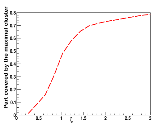
Figure 8: Fraction of the total interaction area covered by the maximal cluster as a function of $\xi$ [47].

2.4 Distribution in the transverse momentum and quenching

Clusters of strings may take quite complicated forms in the transverse plane varying from a disc corresponding to the simple string to long chains of such discs. The question arises what the distribution in transverse momenta of emitted partons will be from a cluster. As we have seen in Subsection 2.2 the average transverse momentum from a cluster can be determined in a comparatively simple manner, especially in the thermodynamic limit:

$${\Big{\langle}}p_{t}^{2}{\Big{\rangle}}={\Big{\langle}}p_{t}^{2}{\Big{\rangle}}_{1}/F(\xi).$$ (74)

However this does not fix the distribution in $p_{t}$ uniquely.

Let us return to our simple picture of the fusion of two simple strings Fig. 6. We assume that partons are emitted independently from the three areas, corresponding to the overlap and two remaining areas. Each of these areas can be visualized as a set of strings of elementary transverse area $d^{2}r$. The total transverse momentum distribution from these three areas will be given by the sum of the three integrals

$$\frac{dp^{tot}}{dyd^{2}p}=C\Big{\{}\int_{S^{(1)}\oplus S^{(3)}}d^{2}re^{-\frac{m_{\perp}^{2}}{t_{1}}}+\sqrt{2}\int_{S^{(2)}}d^{2}re^{-\frac{m_{\perp}^{2}}{t_{1}\sqrt{2}}}\Big{\}}$$

$$=C\Big{\{}2S^{(1)}e^{-\frac{m_{\perp}^{2}}{t_{1}}}+\sqrt{2}S^{(2)}e^{-\frac{m_{\perp}^{2}}{t_{1}\sqrt{2}}}\Big{\}}$$ (75)

and the distribution of emitted particles from the cluster will be

$$I(y,p)=\frac{1}{\mu}\,\frac{dp^{tot}}{dyd^{2}p}=C\frac{2S^{(1)}e^{-\frac{m_{\perp}^{2}}{t_{1}}}+\sqrt{2}S^{(2)}e^{-\frac{m_{\perp}^{2}}{t_{1}\sqrt{2}}}}{2S^{(1)}+\sqrt{2}S^{(2)}}.$$ (76)

Generalizing to many clusters made of different number of simple strings we find the transverse momentum distribution in the general case.

$${\Big{\langle}}p_{t}^{2}{\Big{\rangle}}=C\frac{\sum_{n=1}\sqrt{n}(S_{n}^{tot}/S_{1})e^{-m_{\perp}^{2}/(t_{1}\sqrt{n})}}{\sum_{n=1}\sqrt{n}(S_{n}^{(tot}/S_{1})}.$$ (77)

We recall that $S_{n}^{tot}$ is the total area of overlaps of $n$ simple strings.

We stress that the distribution from the clusters remains isotropic in the transverse space in spite of the fact that clusters themselves have different forms and their distribution may not be isotropic at all.

Equation (77) may be used in the Monte-Carlo simulation. For many practical problems it can be calculated in the thermodynamic limit

$${\Big{\langle}}p_{t}^{2}{\Big{\rangle}}=C\frac{{\Big{\langle}}\sqrt{n}e^{-m_{\perp}^{2}/(t_{1}\sqrt{n})}{\Big{\rangle}}}{{\Big{\langle}}\sqrt{n}{\Big{\rangle}}},$$ (78)

where averaging is done with the Poissonian distribution Eq. (13). With reasonable accuracy it may be further simplified to

$${\Big{\langle}}p_{t}^{2}{\Big{\rangle}}=Ce^{-\frac{m_{\perp}^{2}}{t_{1}{\Big{\langle}}\sqrt{n}{\Big{\rangle}}}},$$ (79)

which implies that the distribution has the same Gaussian form as for a simple string with appropriately enhanced tension.

Experimental data indicate however that the transverse momentum spectra of emitted particles are not isotropic. Their dependence on azimuthal angle together with the anisotropy of the string distribution leads to the well-known azimuthal flows (Section 3.3). In view of this fact our string picture requires certain refinement. As a source of azimuthal anisotropy one may introduce quenching of produced partons in the external chromoelectric field created by strings.

Turn again to fusion of two strings (Fig. 6). Let the observed parton be emitted in different azimuthal directions either from the overlap or from the remaining part of one of the strings (Fig. 9). It is clear that the emitted partons have to travel paths of different longitude before they go out and are observed. Besides, partons going through the overlap meet stronger field than those going only through the field of simple strings. So one concludes that if partons loose their energy passing through the field their observed distribution will depend on their azimuthal angle although initially they were emitted isotropically.

Figure 9: Emission of particles in different azimuthal directions from two overlapping strings.

This implies that the distribution in the transverse momentum has the form Eq. (37) with $p\to p_{0}$ where $p_{0}({\bf p})$ is the parton momentum at the instant of its creation and ${\bf p}$ is the observed momentum

$$P({\bf p})=Ce^{-\frac{p_{0}({\bf p})^{2}}{t}}.$$ (80)

The dependence of $p_{0}({\bf p})$ on the observed momentum will depend both on the longitude of the path traveled by the parton and on the strength of the field it meets along this path. The concrete form of this dependence is determined by the mechanism of quenching.

Radiative energy loss has been extensively studied for a parton passing through the nucleus or quark-gluon plasma as a result of multiple collisions with the medium scattering centers  [98, 99]. In our case the situation is somewhat different: the created parton moves in the external gluon field inside the string. In the crude approximation this field can be taken as being constant and orthogonal to the direction of the parton propagation. In the same spirit as taken for the mechanism of pair creation, one may assume that the reaction force due to radiation is similar to the one in the QED when a charged particle is moving in the external electromagnetic field. This force causes a loss of energy, which for an ultra-relativistic particle is proportional to [its momentum $\times$field]^2/3  [100]:

$$\frac{dp(x)}{dx}=-0.12e^{2}\Big{(}eEp(x)\Big{)}^{2/3},$$ (81)

where $E$ is the external electric field. Eq. (81) leads to the quenching formula

$$p_{0}(p,l)=p\Big{(}1+\kappa p^{-1/3}t^{2/3}l\Big{)}^{3},$$ (82)

where we identified $eE/\pi=t$ as the string tension and $l$ is the longitude of the path traveled by the parton in the field with tension $t$. The quenching coefficient $\kappa$ has to be adjusted to the experimental data. In our practical calculations it was chosen to give the experimental value for coefficient $v_{2}$ in mid-central Au-Au collisions at 200 GeV, integrated over the transverse momenta.

Of course the possibility to use electrodynamics formulas for the chromodynamic case may raise certain doubts. However in  [101] it was found that at least in the $N=4$ SUSY Yang-Mills case the loss of energy of a colored charge moving in the external chromodynamic field was given by essentially the same expression as in the QED.

Note that from the moment of particle creation to the moment of its passage through other strings a certain time elapses depending on the distance and particle velocity. During this time strings decay and the traveling particle will meet another string partially decayed, with a smaller color $Q$ than at the moment of its formation. So one has to consider a non-static string distribution with string colors evolving in time and gradually diminishing until strings disappear altogether. To study the time evolution of strings we again turn to the Schwinger mechanism. For it one has the probability of pair creation in unit time and unit volume as  [102]

$$\Gamma_{VT}=\frac{1}{4\pi}t^{2}e^{-\frac{p_{0}^{2}}{t}},$$ (83)

where again $t$ stands for $eE/\pi$ in QED. For a realistic string the volume $V=SL_{z}$ where $S$ is the string transverse area and $L_{z}$ is the longitudinal dimension of the string. For the single string of color $Q$ we have $t=Qt_{1}$ where $t_{1}$ is the string tension of the ordinary string with $Q=1$. The average transverse momentum squared of the emitted quark-antiquark pair $<p_{0}^{2}>$ is just $t$. To estimate $L_{z}$ we assume that the string emits a pair when its energy is equal to $2<p_{0}>=\sqrt{t}$, which gives $L_{z}=1/\sqrt{t}$, so that we get the average probability in unit time

$$\Gamma_{T}=\frac{1}{4\pi}t^{3/2}S.$$ (84)

The string color diminishes by unity with each pair production. So we find an equation which describes the time evolution of the string color $Q(T)$

$$\frac{dQ(T)}{dT}=-\alpha Q^{3/2}(T)$$ (85)

with the solution

$$Q(T)=\frac{Q_{0}}{(1+\frac{1}{2}\alpha T\sqrt{Q_{0}})^{2}},$$ (86)

where $Q_{0}$ is the initial color at the moment of the string creation. Coefficient $\alpha=t_{0}^{3/2}S/(2\pi)$ depends on the string transverse area $S$. In practical calculations we use the picture in which the fused string is in fact modeled by a set of “ministrings” formed at intersections of simple strings with the same area as the simple string, but greater color. This gives $\alpha=0.03$ $fm^{-1}$. The average color of ministrings is of the order 2 - 3. So it changes only by 30 -50 % even when the emitted parton travels 5 $fm$ of distance. So the time scale of string evolution is estimated to be considerably greater than time intervals characteristic for partons traveling inside the string matter. However the effect of string decay with time is noticeable and we take it into account in our calculations. In fact it practically does not change the results but changes the value of the quenching coefficient $\kappa$, which in any case is to be adjusted, as explained above. In this sense our results are practically independent of the concrete choice of $\alpha$ in the reasonable interval of values.

Finally we note that the Schwinger formula Eq. (37) describes well the spectra only at very soft $p_{0}$. To extend its validity to higher momenta one may use the idea that the string tension fluctuates, which transforms the Gaussian distribution into the thermal one  [103, 104]:

$$P({\bf p})=Ce^{-\frac{p_{0}({\bf p})}{\sqrt{t/2}}}.$$ (87)

2.5 Rapidity dependence

Color strings are stretched between partons into which colliding hadrons or nuclei pass before collisions. Let CM energy squared of the collision be $s=2p\bar{p}\simeq 2p_{+}\bar{p}_{-}$ where $p$ and $\bar{p}$ are the 4-momenta of colliding nucleons and we neglect here the nucleon mass $m$ at high energies. A string carries a fraction of $s$ depending on the momenta of the partons $k$ with $k_{+}=x_{+}p_{1}$ and $\bar{k}$ with$\bar{(}k)=x_{-}\bar{p}$, so that its CM energy squared is $s_{s}=sx_{+}x_{-}$. Defining upper and lower rapidities as

$$y=\frac{Y}{2}+\ln x_{+},\ \ \bar{y}=-\frac{Y}{2}-\ln x_{-}$$ (88)

where $Y=\ln(s/m^{2})$ is the overall rapidity one can say that the string is stretched in the final interval of rapidity between $\bar{y}$ and $y$. If this interval is large then the probability of particle emission at rapidity $y_{p}$ from the string will be practically independent of rapidity while $\bar{y}<y_{p}<y$. This does not imply that the observed particle spectrum will be rapidity independent. In fact, as explained in Section 1.5, partons forming the string are distributed in the colliding hadrons with probabilities $\rho(y)$ and $\rho(\bar{y})$, which are obtained from Eq. (23) upon integration over spectator variables. The final distribution in rapidity $y_{p}$ will then be governed by the factor

$${\cal P}(y_{p})=\int_{y_{p}}^{Y}dy\int_{\bar{y}}^{y_{p}}d{\bar{y}}\rho(y){\rho}(\bar{y}).$$ (89)

and is thus totally determined by the distribution of partons in the colliding hadrons.

Now let us consider string fusion. Let two strings be stretched between partons from the projectile with momenta $k_{1}$ and $k_{2}$ and target momenta $\bar{k}_{1}$ and $\bar{k}_{2}$ with $k_{i+}=x_{i+}p$ and $\bar{k}_{i-}=x_{i-}$, $i=1,2$. Conservation of momentum dictates that if the two strings completely fuse then the ends of the fused string have light-cone momenta $(x_{1+}+x_{2+})k_{+}$ and $(x_{1-}+x_{2-})\bar{k}_{-}$. In terms of rapidities the new ends will be

$$y_{fused}=\ln\Big{(}e^{y_{1}}+e^{y_{2}}\Big{)},\ \ \bar{y}_{fused}=-\ln\Big{(}e^{-\bar{y}_{1}}+e^{-\bar{y}_{2}}\Big{)}$$

where $y_{i}$ and $\bar{y}_{i}$, $i=1,2$ are ends of the fusing strings. This result trivially generalizes to fusion of arbitrary number of strings. If end rapidities of the strings are $y_{i}$ and $\bar{y}_{i}$ then if they completely fuse the ends of the fused string will be

$$y_{fused}=\ln\Big{(}\sum_{i}e^{y_{i}}\Big{)},\ \ \bar{y}_{fused}=-\ln\Big{(}\sum_{i}e^{-\bar{y}_{i}}\Big{)}$$

For illustration, if all the fusing strings are the same then

$$y_{fused}=y+\ln n,\ \ \bar{y}_{fused}=\bar{y}-\ln n$$

The situation obviously complicates if strings are not fused completely, as in Fig. 6. Then one has to consider the three parts with areas $S^{(1)},S^{(2)}$, and $S^{(3)}$ as independent strings and for each of them determine ends in rapidity separately taking into account the sum of the parton momenta in each of the three.

3 Model Results and comparison with experiments

3.1 Multiplicity distributions

The multiplicity distributions in the DPM or QGSM in pp and AA collisions are given by Eqs. (20-21) and Eqs. (35-36) respectively. However, as the energy or the centrality of the collision increases one expects interaction among the strings stretched between the projectile and target partons. As discussed earlier, due to the randomness of the color field in color space, the strength of the resulting color field in a cluster of $n$ strings, is only $\sqrt{n}$ times the strength of the color field of a single string, giving rise to a suppression of the multiplicity of particles produced in the decay of the cluster. The same reason lies at the origin of the enhancement of the mean transverse momentum with string density. The corresponding equations for both quantities, were obtained in the previous section, Eq. (49) and Eq. (74) respectively.

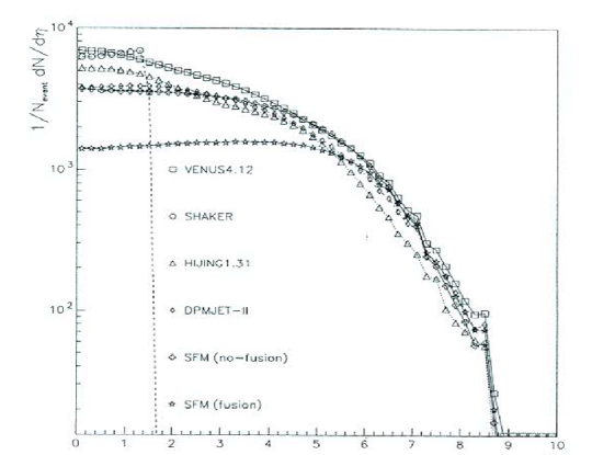
Figure 10: Pseudorapidity distribution of charged particles for central Pb-Pb events at a beam energy of 3 TeV per nucleon [105].

At present, most of the models have incorporated the suppression of multiplicities compared with the superposition of independent scatterings result by means of different mechanisms, but this was not so twenty years ago, when the predictions of all the models for central Pb-Pb collisions at LHC energy were a factor two higher than the prediction of the string fusion model (SFM) [94, 105], which was a previous version of the percolation string model, as it is seen in Fig. 10. The SFM prediction is close to the LHC data for Pb-Pb collisions at 2.76 TeV. According to Eq. (49) the multiplicity distribution in pp collisions in the central rapidity region is given by

$$\frac{dN^{pp}}{dy}=F(\xi_{p})N_{p}^{S}\mu_{1},\ \ \xi_{p}=N_{p}^{s}\frac{S_{1}}{S},$$ (90)

where factor $F$ is given by Eq. (51), $N_{P}^{S}$ is the number of strings in the central rapidity region, $S_{1}=\pi r_{0}^{2}$ with $r_{0}=0.2$ fm and $S$ is the transverse area of the proton. In the DPM in nucleus-nucleus collisions the number of strings stretched between the sea quark and antiquarks in the central rapidity region is proportional to $N_{A}^{4/3}-N_{A}$ and is given by Eq. (36). Here $N_{A}^{4/3}$ is the total number of nucleon-nucleon collisions. Hence, the total number of strings in a central heavy ion collisions can be very large, actually more than $\sim 10^{3}$ strings are produced in Au-Au at RHIC energies. However, each string must have a minimum of energy to be produced and decay subsequently into particles (at least two pions). On the other hand, the total energy available in a collision grows as $A$, whereas the number of strings $\sim A^{4/3}$ in central collisions. Hence, at not very high energy (for instance RHIC energy) the energy is not sufficient to produce such a large number of strings. In order to take into account this energy momentum conservation effect one may reduce the number of sea quark and antiquark strings, changing [106]

$$N_{A}^{4/3}\rightarrow N_{A}^{1+\alpha(\sqrt{s})}$$ (91)

with

$$\alpha(\sqrt{s})=\frac{1}{3}\Big{(}1-\frac{1}{1+\ln(\sqrt{(}s/s_{0})+1)}\big{)}.$$ (92)

One can thus write

$$\frac{dN^{AA}}{dy}\sim N_{A}(N_{A}^{\alpha(\sqrt{s})-1})\frac{dN^{pp}}{dy}.$$ (93)

Parameter $s_{0}$ marks the energy squared below which energy-momentum conservation effects become small and $\alpha\rightarrow$1/3. Up to here we do not take into account the interaction among the strings. If we do take into account the interaction of strings then we can write a closed formula for the multiplicity distribution in $AA$ collisions in terms of the multiplicity distribution in pp collisions, namely [106]

$$\frac{1}{N_{A}}\frac{dN}{dy}{\Big{|}}_{y=0}=\frac{dN^{pp}}{dy}{\Big{|}}_{y=0}\Big{(}1+\frac{F(\xi_{N_{A}})}{F(\xi_{p})}N_{A}^{\alpha(\sqrt{s})-1}\Big{)}$$ (94)

where

$$\xi_{N_{A}}=\xi_{p}N_{A}^{\alpha(\sqrt{s})+1}\frac{S_{1}}{S_{N_{A}}}$$ (95)

and $S_{N_{A}}$ is the transverse area of the collision region formed when there are $N_{A}$ wounded nucleons of the projectile and $N_{A}$ nucleons of the target. $S_{N_{A}}$ depends on $N_{A}$ and A. The dependence of the multiplicity on the center of mass collision energy $\sqrt{s}$ is fully specified once the average number of strings in a pp collision $N_{p}^{s}$ is known. At low energy $N_{p}^{s}$ is approximately equal to 2, growing with energy as $(\sqrt{s}/m_{p})^{2\lambda}$ so that

$$N_{p}^{s}=2+4(\frac{r_{0}}{R_{p}})^{2}(\frac{\sqrt{s}}{m_{p}})^{2\lambda}.$$ (96)

Here a single parameter $\lambda$ describes the rise of the multiplicity with energy for both pp and AA multiplicity distributions, even though in AA central collisions the multiplicity increases faster than in pp collisions due to the energy dependent factor $\alpha$, arising from energy momentum conservation.

A fit to pp collisions data in the range 53 $\leq\sqrt{s}\leq$ 7000 GeV and to AA collisions (Au-Au, Cu-Cu, and Pb-Pb) at different centralities for 19.6 $\leq\sqrt{s}\leq$ 2760 GeV has been done. The values obtained from the fit for the two parameters are $\sqrt{s}_{0}$ = 245 GeV and $\lambda$ =0.201.

Figure 11 shows a comparison of the results for the dependence of midrapidity multiplicity on the energy with data for pp [107, 108, 109, 110, 111, 112, 113] and central Cu-Cu ($N_{A}$ = 50, A = 63) [114] and for Au-Au/Pb-Pb ($N_{A}$ = 175, A = 200) [115].

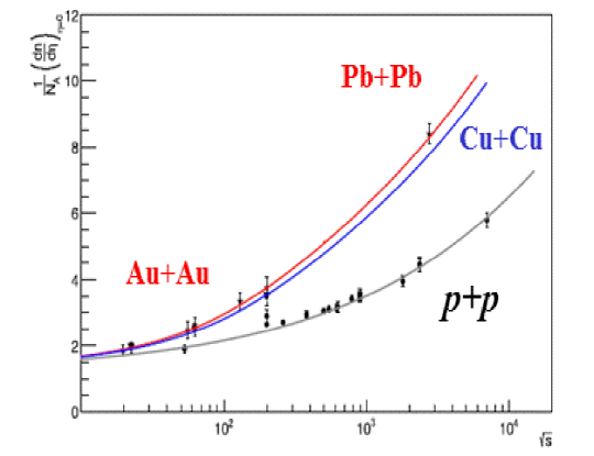
Figure 11: Comparison of the evolution of the mid-rapidity multiplicity with energy from the CSPM and data for pp and A-A collisions. Lines are from the model for pp (gray), Cu-Cu (blue) and red lines for Au-Au/Pb-Pb [106].

In Fig. 12 the result of the dependence of the multiplicity per participant nucleon on the number of participants is shown together with the experimental data for Cu-Cu ($\sqrt{s_{NN}}$ = 22.4, 62.4, 200 GeV) for Au-Au ($\sqrt{s_{NN}}$= 19.6, 62.4, 130 and 200 GeV) and for Pb-Pb ($\sqrt{s_{NN}}$ = 2.76, 3.2, 3.9, 5.5 TeV).

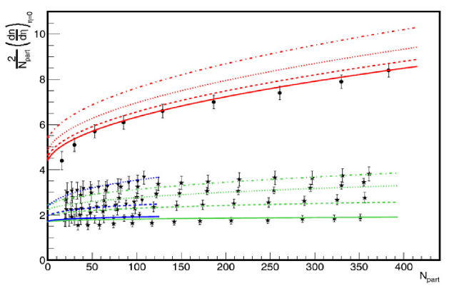
Figure 12: Multiplicity dependence on centrality ($N_{part}$). Cu-Cu (triangles), Au-Au (stars) and Pb-Pb (circles).Curves represent the model calculations. Blue line for Cu-Cu, green line for Au-Au and red for Pb-Pb [106].

The evolution outside the central rapidity region has been studied extensively extending to all rapidities Eq. (96) [116, 117, 118, 119]:

$$\frac{1}{N_{A}}\frac{dN^{N_{A}N_{A}}}{d\eta}=KJF(\xi_{p})N_{p}^{s}\frac{\Big{(}1+\frac{F(\xi_{N_{A}})}{F(S_{p})}(N_{A}^{\alpha}-1)\Big{)}}{\exp\Big{(}\frac{(\eta-(1-\alpha)Y)}{\delta}\Big{)}+1},$$ (97)

where $J$ is the Jacobean

$$J=\frac{\cosh\eta}{\sqrt{k_{1}+\sinh^{2}\eta}}$$

and

$$K=\frac{k}{J(\eta=0)}\Big{(}\exp(\frac{-(1-\alpha)Y}{\delta})+1\Big{)}.$$ (98)

Parameters $\alpha$ and $\delta$ are obtained from fitting to the data ($\alpha=0.34,\delta=0.84$). The pseudorapidity dependence is described by the same factor

$$\frac{1}{\exp(\frac{\eta-(1-\alpha)Y}{\delta})+1}$$ (99)

in pp and AA collisions. This dependence gives rise to a smaller increase at central pseudorapidity $\eta$ = 0 than at large pseudorapidity $\eta$ = Y [117, 118]. The limiting fragmentation property have been studied carefully, showing it is not exact and a violation of it should be more visible at the highest LHC energies [116, 117, 118]. In Fig. 13 we show the comparison of Eq. (97) with experimental data at different energies (53 GeV $\leq\sqrt{s}\leq$ 7 TeV) [120, 121]. In Fig. 14(a-c) we show the comparison between the results for Cu-Cu [121], Au-Au [122] and Pb-Pb [123] collisions and the experimental data.

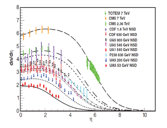
Figure 13: Comparison of results from the evolution of $dn_{ch}/d\eta$ with dependence on pseudorapidity for pp collisions at different energies (lines) [119].

The percolation of strings have been applied to the case of different projectile and target as well. In Fig. 14(d) the results for d+Au at different centralities compared to the experimental results [17] are shown. Similar results were obtained in Ref. [124].

The behavior obtained for $dN/dy$ in pp and AA collisions with energy and number of participants is very similar to the Glasma picture in CGC. In fact, in CGC the multiplicity distribution is given by  [41]

$$\frac{dN}{dy}\sim\frac{1}{\alpha_{s}(Q_{s})}Q_{s}^{2}R_{A}^{2}.$$ (100)

Since the saturation momentum squared $Q_{s}^{2}$ behaves like $N_{A}^{1/3}$, the multiplicity per participant is almost independent of $N_{A}$ and a weak dependence arises from the logarithmic dependence on $N_{A}$ of the running coupling constant $1/\alpha_{s}\sim\log N_{A}$. In percolation the multiplicity per participant is almost independent of $N_{A}$ as well and the only additional dependence arises from the factor $(1-\exp(-\xi))^{1/2}$ which grows weakly with $N_{A}$ above the percolation threshold. Concerning the energy dependence, $Q_{s}^{2}$ behaves like $s^{\lambda}$, so that the same behavior is obtained in percolation. There is an extra energy dependence due to the running coupling constant $\alpha_{s}(Q_{s})$ in the CGC, which again corresponds to the energy dependence of the factor $(1-\exp(-\xi))^{1/2}$. It is not surprising that their exist a correspondence between 1/$\alpha_{s}$, the occupation number or the number of gluons, and the factor $1-\exp(-\xi)$ which represents the fraction of the collision area covered by strings. The larger the occupation number the larger the fraction is. The similarities between the Glasma picture of CGC and the percolation of strings are visible not only in multiplicities but in most of the other observables, as discussed later.

In order to explain the faster rise of the multiplicity in central AA collisions than in pp collisions several possibilities have been proposed in CGC, such as enhanced parton showers in AA collisions due to the larger average transverse momentum of the initially produced minijets compared to pp collisions [125] or non trivial Q effects intertwined with impact parameter dependence [126].

3.2 Transverse momentum distributions

In Section 2.4 we studied the effects of percolation of strings on the mean transverse momentum and the dispersion of the transverse momentum distribution and the experimental data related to it.

As explained in Sec. 2 the detailed study of both multiplicity and momentum distribution requires analysis of all overlaps of created strings which differ both in the number of the strings in the overlap and in the area of a particular overlap. With a large number of strings created in AA collisions at high energy this is hardly feasible. So it is reasonable to search for some effective way to describe the observables in this situation.

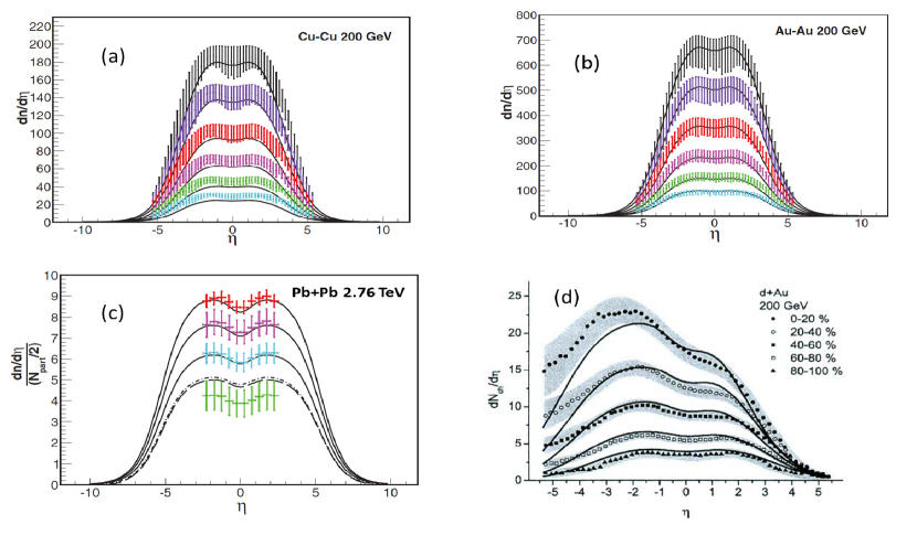
Figure 14: Comparison of results from the evolution of $dn_{ch}/d\eta$ with dependence in pseudorapidity for (a).Cu-Cu at 200 GeV, (b) Au-Au 200 GeV. Plot (c) show $\frac{dn_{ch}}{d\eta}\frac{1}{(N_{part}/2)}$ for Pb-Pb collisions at 2.76 TeV (d) dn/d$\eta$ at different centralities for d+Au collisions at 200 GeV [119].

Let us start with multiplicities. They come from a set of overlaps (“ministrings”) and depend on both the number of overlapped strings and the area of the overlap, which combine to give an average multiplicity $N$ from this overlap. We may characterize different overlaps just by this average multiplicity. We call $N$ a “size” of the overlap, the quantity combining both the number of overlapped strings and the area. With a lot of overlaps $N$ will be changing practically continuously. We then can introduce a probability $W(N)$ to have overlaps with size $N$ in a collision and write the total distribution in multiplicity as

$$P(n)=\int dNW(N)P(N,n),$$ (101)

where $P(N,n)$ is the multiplicity distribution from the overlap of a given $N$, which we take to be Poissonian with the average multiplicity $N$

$$P(N,n)=\exp(-N)N^{n}/n!.$$ (102)

The normalization conditions $\sum_{n}P(n)=\sum_{n}P(N,n)=1$ and the condition $\sum_{n}nP(N,n)=N$ lead to relations

$$\int dNW(N)=1,\ \ <n>=<N>=\int dNNW(N).$$ (103)

For the weight function we assume the gamma distribution [127, 128, 129]

$$W(N)=G(N,k_{N},r_{n})=\frac{r_{N}}{\Gamma(k_{N})}(r_{N}N)^{k_{N}-1}\exp(-r_{N}N),r_{N}=\frac{k_{N}}{<N>}.$$ (104)

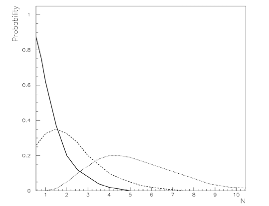
Figure 15: Schematic representation of the number of clusters as a function of the number of strings of each cluster at three different centralities [128].

There are several reason for this choice. First, the gamma distribution reproduces to a good approximation the cluster size distributions at different centralities. In fact, let us consider a peripheral collision, where the density of strings is small and there are only very few overlapping strings. In this case, the cluster size is peaked at low values of the number of strings of the cluster. As the centrality increases, the density of strings increases as well ,and there are more and more overlapping strings. The cluster size distribution becomes strongly modified. Figure 15 shows a plot of three different cluster size distributions corresponding to three centralities. Each one can be described by a gamma function corresponding to different values of $k_{N}$.

There is another reason for choosing the gamma function, related to the re-normalization group. The growth of the centrality can be seen as a transformation of the cluster size distribution. Start with a set of single strings with a few clusters formed of a few overlapping strings. As the centrality increases, there appear more strings and more clusters composed of more strings. This change can be considered as substitution of strings in a cluster by newly formed clusters, defined by new $<n>$, corresponding to a higher color field in the cluster. This transformation, similar to the block transformations of Wilson type, can be seen as a transformation of the cluster size probability of the type:

$$P(x)\rightarrow\frac{xP(x)}{<x>}....\rightarrow\frac{x^{k}P(x)}{<x^{k}>}\rightarrow...$$ (105)

Transformations of this kind were studied long time ago by Jona-Lasinio in connection with the re-normalization group in probability theory [130], showing that the only probabilities $P(x)$ stable under such transformations are the generalized gamma functions. Among the generalized gamma functions the simplest one is the gamma function which in addition has one parameter less (This additional parameter could be used to refine the model for comparison with the data). The transformations of type Eq. (105) have been used previously to study the probability associated with some special events which are shadowed only by themselves and not for the total of events [131, 132, 133, 134, 135].

Notice that $W(N)$ satisfies KNO scaling, namely the product $NW(N)$ is only a function of $N/<N>$ and not of the energy. This property is a consequence of the invariance of the form of the gamma functions under transformations of type Eq. (105) [136].

Now we pass to the transverse momentum distribution (TMD) $f(p_{t})$. As in the case of multiplicities it comes from overlaps of different number of strings having different areas and the TMD from an overlap depends on its both characteristics (we may again call this combination a “size” of the overlap, this time in respect to the TMD). Take the TMD from an overlap of a given size given by the Schwinger mechanism

$$f(p_{t},x)=\exp(-xp_{t}^{2})$$ (106)

where $x$ is just this “size”. Assuming again that $x$ varies continuously one can write the total TMD, in all similarity to Eq. (101), as

$$f(p_{t})=\int dxW_{p}(x)f(x,p_{t})$$ (107)

with a certain positive weight $W_{p}(x)$. To understand its property we use the normalization condition for TMD

$$\int dp_{t}^{2}f(p_{t})=<n>$$ (108)

This gives a relation

$$\int\frac{dx}{x}W_{p}(x)=<n>.$$ (109)

On the other hand, introducing integration variable $N=\alpha x$ we have from Eq. (103)

$$<n>=\int dxx\alpha^{2}W(\alpha x).$$ (110)

Comparing this with Eq. (109) we can make an identification

$$W_{p}(x)=(\alpha x)^{2}W(\alpha x)$$ (111)

If we take the gamma distribution Eq. (104) for $W(N)$ then $W_{p}(x)$ turns out up to a factor to be also the gamma distribution bit with different $k$ and $r$

$$W_{p}(x)=\frac{r}{r_{p}}G(x,k+2,r_{p})$$ (112)

with $r_{p}=\alpha r$ (note that $\alpha$ is dimensionful).

So in the end both the distribution $P(n)$ and TMD $f(p_{t}^{2})$ are given by a convolution of the cluster multiplicity and its TMD with the size probability $W$, which in both cases can be taken as the gamma distribution although with different parameter $k_{N},r_{N}$ and $k_{p},r_{p}$ respectively. In the following having in mind that most applications will be devoted to the TMD, we denote $k_{p}$ and $r_{p}$ as simply $k$ and $r$ leaving notations $k^{\prime}$ and $r^{\prime}$ for $k_{N}$ and $r_{N}$. In many discussions the behavior of $k$ and $k^{\prime}$ is similar and we do not specify which of the two $k$’s we are discussing.

Introducing Eq. (104) into Eq. (107) and Eq. (101), we obtain

$$\frac{1}{(1+\frac{P_{t}^{2}}{r})^{k}}=\int_{0}^{\infty}dx{\exp(-p_{t}^{2}x)(\frac{r}{\Gamma(k)})(rx)^{k-1}\exp(-rx)}$$ (113)

and

$$\frac{\Gamma(n+k^{\prime})}{\Gamma(n+1)\Gamma(k^{\prime})}\frac{r^{`k}}{(1+r{{}^{\prime}})(n+k^{\prime})}$$

$$=\int_{0}^{\infty}dN\frac{e^{N}N^{n}}{n!}\frac{r^{{}^{\prime}}}{\Gamma(k^{\prime})}(r^{{}^{\prime}}N)^{k^{\prime}-1})\exp(-r^{{}^{\prime}}N).$$ (114)

The mean value and the dispersion of the distributions Eq. (113) and Eq. (114) are

$$<x>=\frac{k}{r},\frac{<x^{2}>-<x>^{2}}{<x>^{2}}=\frac{1}{k}$$ (115)

$$<n>=<N>\frac{k^{\prime}}{r^{{}^{\prime}}},\ \ \frac{<N^{2}>-<N>^{2}}{<N>^{2}}=\frac{1}{k^{\prime}},$$ (116)

$$\frac{<n^{2}>-<n>^{2}>}{<n>^{2}}=\frac{1}{k^{\prime}}+\frac{1}{<N>}$$ (117)

The distribution given by Eq. (113) is the negative binomial distribution. Equations (113) and (114) can be seen as a superposition of sources (clusters) where $1/k$ and $1/k^{\prime}$ fix the transverse momentum fluctuations and the fluctuations on the number of strings in the clusters. At small string density there are almost no strings overlapped, the strings are isolated and $k$ and $k^{\prime}$ tend to infinity. When the density increases, there will be some overlapping strings forming clusters, and therefore $k$’s decrease. Their minimum is reached when fluctuations in the number of strings per cluster reach their maximum. Above this point, with increasing string density, these fluctuations decrease and $k$’s increase. We recall that $k$ and $k^{\prime}$ are generally different. When comparing to the experimental data to fix them, one also has to take into account the experimental conditions, such as acceptance and range of variables studied.

Now we have to take into account that the mean transverse momentum and mean multiplicity of a cluster of strings is given by Eqs. (49) and (74) and therefore we should incorporate this into Eqs. (113) and (114). In this way the respective distributions become

$$f(p_{t},y)=\frac{dN}{dp_{t}^{2}dy}=\frac{dN}{dy}\frac{k-1}{k}\frac{F(\xi)}{<p_{t}^{2}>_{1}}\frac{1}{\Big{(}1+\frac{F(\xi)p_{t}^{2}}{k<p_{t}^{2}>_{1}}\Big{)}^{k}}$$ (118)

and

$$P(n)=\frac{\Gamma(n+k^{\prime})}{\Gamma(n+1)\Gamma(k^{\prime})}\frac{\Big{(}\frac{k^{\prime}}{<n>_{1}F(\xi)}\Big{)}^{k^{\prime}}}{\Big{(}1+(\frac{k^{\prime}}{<n>_{1}F(\xi)})\Big{)}^{n+k^{\prime}}}$$ (119)

We observe that

$$<n>=F(\xi)N_{s}<n>_{1},\ \ <p_{t}^{2}>=\frac{k}{k-2}\frac{<p_{t}^{2}>_{1}}{F(\xi)}$$ (120)

Equations (118) and (119) give the distributions for any projectile, target, energy and degree of centrality and are universal functions which depend only on two parameters $<p_{t}^{2}>_{1}$ and $<n>_{1}$ the transverse momentum and multiplicity of particles produced by one string. In the case of identified secondary particles the corresponding quantities for each identified particle, $<p_{t}^{2}>_{1i}$ and $<n>_{1i}$ should be used. In addition to these parameters, parameters $k$ and $k^{\prime}$, actually are functions of centrality and, as we said above, with the growth of string density first decrease up to a minimum close to the critical percolation value and afterwards increase . At $\xi\rightarrow\infty,k\rightarrow\infty$ and the distribution given by Eq. (118) becomes $\exp(-F(\xi)p_{t}^{2}/<p_{t}^{2}>_{1})$ very similar to the behavior at $\xi\rightarrow 0$. From Eq. (118) we have.

$$\frac{dlnf}{dlnp_{t}}=\frac{-2F(\xi)}{\Big{(}1+\frac{F(\xi)p_{t}^{2}}{k<p_{t}^{2}>_{1i}}\Big{)}}\frac{p_{t}^{2}}{<p_{t}^{2}>_{1i}}.$$ (121)

At $p_{t}^{2}\rightarrow 0$ this reduces to $-2F(\xi)p_{t}^{2}/<p_{t}^{2}>_{1i}$ and vanishes at $p_{t}$ = 0. On the other hand, as the mean $p_{t}$ of particles produced in a single string is larger for protons than for kaons and the latter larger than for pions, $<p_{t}^{2}>_{1\pi}$ $<$ $<p_{t}^{2}>_{1k}$ $<$ $<p_{t}^{2}>_{1p}$, the absolute value of the left-hand side of Eq. (121) is larger for pions than for kaons and than for protons. This is the well known hierarchy that is very often advocated as evidence in favor of hydrodynamics models. In Fig. 16 the results of our distribution Eq. (118) are shown compared to the RHIC data of PHOBOS  [137] for central Au-Au collisions at $\sqrt{s_{NN}}$ = 200 GeV. We use the values $<p_{t}^{2}>_{1\pi}=0.06,<p_{t}^{2}>_{1k}=0.14,\\ <p_{t}^{2}>_{1p}=0.30$ and $k=4$. The value of the string density is 2.5. We observe a good agreement taking into account that our result is not a fit but the result of Eq. (118) fixing the normalization of the three curves at the same value at $p_{t}$ = 2 GeV/c.

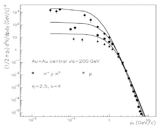
Figure 16: Experimental PHOBOS data on low $p_{t}$ distributions for pions, kaons and protons along with our results for central Au-Au collisions at $\sqrt{s_{NN}}$ = 200 GeV [128].

Let us now discuss the interplay between low and high $p_{t}$. One defines the ratio $R_{CP}(p_{t})$ between central and peripheral collisions as

$$R_{CP}(p_{t})=\frac{f^{{}^{\prime}}(p_{t},y=0)/N_{coll}^{{}^{\prime}}}{f(p_{t},y=0)/N_{coll}},$$ (122)

where the distributions in the numerator and denominator correspond to central and peripheral collisions respectively, $\xi^{{}^{\prime}}>\xi$. The normalization on the number of collisions in Eq. (122), essentially eliminates $N_{s}$, the number of strings, from dN/dy (this is true at midrapidity and not at forward or backward rapidities). From Eqs. (107) and (118) we obtain

$$R_{CP}(p_{t})=\frac{((k^{{}^{\prime}}-1)/k^{{}^{\prime}})}{((k-1)/k)}\Big{(}\frac{F(\xi^{{}^{\prime}})}{F(\xi)}\Big{)}^{2}\frac{\Big{(}1+\frac{F(\xi)p_{t}^{2}}{k<p_{t}^{2}>_{1i}}\Big{)}^{k}}{\Big{(}1+\frac{F(\xi^{{}^{\prime}})p_{t}^{2}}{k^{{}^{\prime}}<p_{t}^{2}>_{1i}}\Big{)}^{k^{{}^{\prime}}}}.$$ (123)

Here $k$ and $k^{\prime}$ are values of the parameter $k$ for transverse momentum distribution for peripheral and central collisions. In the limit $p_{t}^{2}\rightarrow 0$, as $F(\xi^{{}^{\prime}})<F(\xi)$ we obtain

$$R_{CP}(0)\simeq\Big{(}\frac{F(\xi^{{}^{\prime}})}{F(\xi)}\Big{)}^{2}<1,$$ (124)

which is approximately independent of $k$ and $k^{\prime}$. As $\xi^{{}^{\prime}}/\xi$ increases the ratio $R_{CP}$ decreases, in agreement with the experimental data. As $p_{t}$ increases, we have

$$R_{CP}(p_{t})\sim\frac{1+\frac{F(\xi)p_{t}^{2}}{k<p_{t}^{2}>_{1i}}}{1+\frac{F(\xi^{{}^{\prime}})p_{t}^{2}}{k^{\prime}<p_{t}^{2}>_{1i}}}$$ (125)

and $R_{CP}$ increases with $p_{t}$ (again $F(\xi)>F(\xi^{{}^{\prime}})$). At large $p_{t}$

$$R_{CP}(p_{t})\sim\frac{F(\xi)}{F(\xi^{{}^{\prime}})}\frac{k^{{}^{\prime}}}{k}p_{t}^{2(k-k^{\prime})}.$$ (126)

At low density in the region where $k$ decreases with the string density $k^{\prime}<k$ and $R_{CP}(p_{t})>1$. It is the Cronin effect. As $\xi^{{}^{\prime}}/\xi$ increases the ratio $R_{CP}$ increases.

With the growth of the energy of the collision, the energy density increases and therefore we arrive at the region where $k$ increases. Now as $\xi^{{}^{\prime}}>\xi$, $k^{{}^{\prime}}>k$ and there will be a suppression of $p_{t}$.

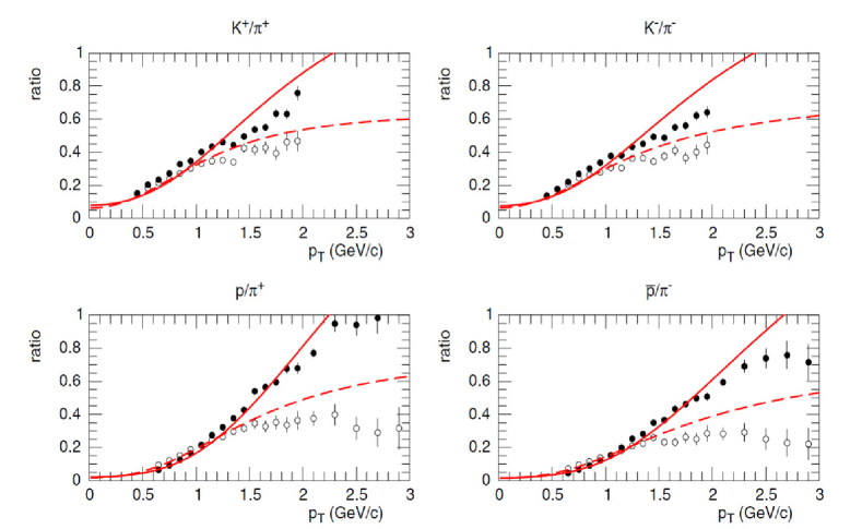
Figure 17: Ratios for different distributions K/$\pi$, p/$\pi$ in Au-Au collisions at $\sqrt{s_{NN}}$ = 200 GeV at two different centralities :(0-5%, solid circles, 60-70-% open circles) in comparison with the data [129].

In the forward rapidity region, the normalization of $N_{coll}$ in Eq. (122) does not cancel $N_{s}$ from $dN/dy$, since in this region $N_{s}$ is proportional to $N_{A}$ instead of $N_{coll}$. Therefore, an additional factor $\frac{N_{A}^{{}^{\prime}}/N_{coll}^{{}^{\prime}}}{N_{A}/N_{coll}}$ appears now in $R_{CP}(p_{t})$. As $N_{coll}^{{}^{\prime}}-N_{A}^{{}^{\prime}}$ for central collision is larger than the corresponding quantity for peripheral collisions, we have $R_{CP}(p_{t},y=3)<R_{CP}(p_{t},y=0)$, thus a further suppression occurs in agreement with the experimental data [138].

The results for the TMD for $\pi^{+},K^{+}$ and p in Au-Au collisions at $\sqrt{s_{NN}}$ = 200 GeV are in good agreement with the PHENIX experimental data [139]. In Fig. 17 we show the ratios kaons/pions and proton/pions as a function of $p_{t}$ at the two extreme centralities compared to the experimental data. The obtained values of $k$ as a function of the string density evaluated for each centrality are shown in Fig. 18. The expected increase of $k$ with the string density is clearly seen.

The experimental data on pp in the range $\sqrt{s}$ =23, 200, 630, 1830, and 70000 GeV can be described by the distribution Eq. (118)  [140] as well. In this case the values of $k$ decrease with energy as expected, a higher energy means a higher string density. Notice that for string densities above the critical percolation value, $k$ should increase, hence in pp a change in the behavior of $k$ is predicted. At 14 TeV the string density would be close to such critical value but probably would not reach it.

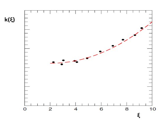
Figure 18: $k(\xi)$ extracted from $\pi^{+}$ fits. The behavior expected in percolation is suggested by the data [129].

Concerning the baryon $p_{t}$ distributions, the difference with the meson spectrum is not only due to the difference of masses which results in that $<p_{t}>_{Mesons}$ $<$ $<p_{t}>_{Baryons}$. This effect only causes a shift of the maximum of the nuclear modified factor $R_{AA}$ but keeps the same height at the maximum contrary to the data. In the fragmentation of a cluster formed by several strings the flavor properties follow from the corresponding properties of the individual strings and hence the resulting flavor of the cluster $F$ is the flavor composition of the individual strings $f$ as well as the color composition. We obtain clusters with higher color and different flavored ends. In the fragmentation of a cluster we consider the creation of a pair of complexes $F\bar{F}$. After the decay the two new $F\bar{F}$ strings are treated in the same way and therefore decay into more $F\bar{F}$ strings until they come to objects with masses comparable to hadron masses, which are identified with observable hadrons by combining the produced flavor with statistical weights. In this way the production of baryons and antibaryons is enhanced. We observe that additional quarks or antiquarks required to form a baryon or antibaryon are provided by the quarks or antiquarks of the overlapping strings that form the cluster. In some sense this coalescence is incorporated in a natural way  [141, 142, 143] in the CSPM. In order to take this into account, keeping a similar formula for the TMD, we modify the latter in an effective way [144]. We take for the multiplicity (per unit rapidity) of baryons and antibaryons.

$$\frac{dN}{dy}=N_{s}^{1+\alpha}F(\xi)<n>_{1B}$$ (127)

instead of Eq. (107) fitting the parameter $\alpha$ to reproduce the experimental data ($\alpha$ =0.09). From Eq. (127) we observe that when a (anti)baryon is triggered the effective number of strings is $N_{s}^{1+\alpha}$ instead of $N_{s}$. This means that the string density $\xi$ must be replaced by $N_{s}^{\alpha}\xi$. The (anti)baryons probe a higher density than the mesons for the same energy. The value of $\alpha$ is different for baryons and antibaryons because the rise with centrality is slightly different for them, depending on the specific kind of baryon or antibaryon as well. In Fig. 19 we plot the results [144] for $R_{CP}$ (0-10% central)/(60-92% peripheral) for pions and ($p+\bar{p}$)/2 compared to PHENIX data. At 5.5 TeV the LHC predictions are shown. In Fig. 19 we plot the antiproton to neutral pion ratio for central and peripheral centrality bins compared to the PHENIX data together with the predictions at 5.5 TeV. More results can be seen in Ref. [145], where the the open charm production has been studied. Related to percolation, there are other extensive studies of the effects of the strong color field on the string tension, including the effect of baryon junction. These studies extend to strangeness production [146, 147] and charm production [148, 149] in pp and AA collisions.

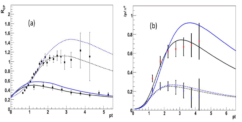
Figure 19: (a)$R_{CP}$ (0-10% central/60-92% peripheral) for pions(solid line) and (p+$\bar{p}$)/2 (dashed) compared to the PHENIX data. Blue line is LHC predictions. (b) $\bar{p}/\pi^{0}$ as a function of $p_{t}$ for 0-10% (solid) and 60-92% (dashed) centrality bins. The points are from PHENIX data. LHC predictions are in blue [144].

Equation (118) for the $p_{t}$ distribution does not include the high $p_{t}$ region as far as we take a Gaussian shape for the fragmentation of a cluster. A more detailed form for the cluster taking into account perturbative QCD for the high $p_{t}$ region may extend the range of validity of our modified distribution.

There are several scaling properties found in the TMD related to string percolation. The experimental data for pp collisions exhibit a universal behavior in a suitable variable $z=p_{t}/K$

$$\phi(z)=A\frac{d^{2}N}{2p_{t}dp_{t}d\eta}|_{p_{t}=Kz}.$$ (128)

Here the parameters $A$ and $K$ depend on the energy of the pp or p$\bar{p}$ collisions. This universal scaling behavior [150], as is shown in Fig. 20 for pp at $\sqrt{s}$ =0.9, 2.36 and 7 TeV and $p\bar{p}$ at 0.63, 1.8, 1.96 TeV. The value of ${\it K}$ increases with the energy. In string percolation this scaling is satisfied by the distribution Eq. (118) with ${\it K}$ proportional to 1/F($\xi$). As F($\xi$) decreases with energy ${\it K}$ increases. A similar scaling has been found in Au-Au [151, 152] at different centralities for the distributions of kinetic energy of pions, kaons and protons. Again the percolation of strings distribution satisfies this scaling.

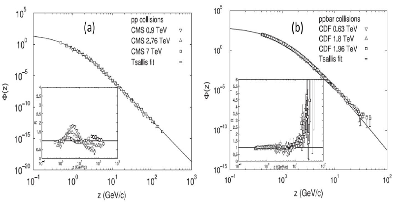
Figure 20: Scaling behavior of the charged hadron $p_{t}$ spectra presented in ${\it{z}}$ (a) in pp collisions and (b) $p\bar{p}$ collisions with different energy scales. The inset is the distribution of the ratio between the experimental data and the fitted results [150].

Recently, it has been shown that in pp collisions the $p_{t}$ spectra of charged particles exhibit geometrical scaling, which is also satisfied in nucleus-nucleus collisions [153, 154]. Using proper normalizations it was shown that in any type of collision for any centrality and energy the different distributions approximately are lying on the same curve for low and moderate $p_{t}$ [155], namely

$$\frac{1}{N_{A}}\frac{dN}{dp_{t}^{2}}=\phi(\tau),\ \ \tau=\frac{p_{t}^{2}}{Q_{s}^{2}}.$$ (129)

This is illustrated in Fig. 21, where the data for pp, pPb, Cu-Cu, Au-Au, and Pb-Pb at different energies and centralities are plotted.

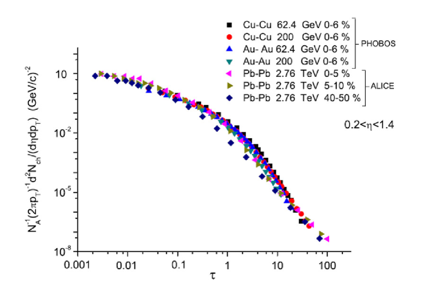
Figure 21: Charged particle multiplicity per participant at pseudorapidity $0.2<\eta<1.4$ for Au-Au and Cu-Cu central collisions at two RHIC energies 62.4 and 200 GeV. and for Pb-Pb collisions at 2.76 TeV plotted as a function of $\tau$ for $\lambda=0.27$ [155].

The percolation of strings, at low $p_{t}$ satisfies this scaling. In fact at low $p_{t}$, the distribution Eq. (118) becomes exp$(-p_{t}F(\xi)/<p_{t}>)$ which is a function only of $p_{t}/Q_{s}$ if $Q_{s}$ is proportional to $<p_{t}>/F^{1/2}(\xi)$.

The experimental data on the mean $p_{t}$ as a function of the multiplicity have shown an interesting systematic in pp, pPb, and Pb-Pb collisions at LHC. All of them grow with multiplicity, being larger in pp than in pPb and in Pb-Pb collisions [156, 157]. On the other hand, in Pb-Pb collisions the rise of mean $p_{t}$ with multiplicity is flattened above a certain low multiplicity. The same occurs for pPb collisions, even though in this case the change of behavior is at higher multiplicity. All this behavior is understood easily in string percolation as a consequence of Eq. (120). In fact factor $1/F^{2}(\xi)$ is responsible for the rise with multiplicity of mean $p_{t}$ because $\xi$ grows with multiplicity. The flattening of the mean $p_{t}$ exhibited in Pb-Pb and pPb data is due to the dependence of the parameter $k$ in Eq. (120) on the string density $\xi$. In Pb-Pb for most of multiplicities the corresponding string densities $\xi$ are above the critical percolation value. In this region, $k$ grows with $\xi$ and the rise of $p_{t}$ is lowered. The same happens in pPb, but now we need higher multiplicities to have string densities above the critical percolation density. In the case of pp collisions most of the corresponding string densities lie below the critical percolation string density. In this region $k$ is a decreasing function of $\xi$, hence there is no flattening. We expect that at higher energies even in pp collisions the critical density will be reached. However at 14 TeV probably the string density will be slightly below. This discussion refers to charged particles but can be extended to identified particles. In the case of baryons, as noted before, there are additional enhancements due to the higher flavor of the cluster. This can be taken into account in an effective way assuming that baryons probe a higher string density. Due to that we expect a flattening of the mean $p_{t}$ of baryons as a function of the multiplicity at future LHC energies.

3.3 Collective flow and ridge

The cluster formed by the strings has generally an asymmetric form in the transverse plane and acquires dimensions comparable to the nuclear overlap. This azimuthal asymmetry is at the origin of the elliptic flow in CSPM. The partons emitted at some point inside the cluster have to pass through the strong color field before appearing on the surface. The energy loss by the parton is proportional to the length and therefore the $p_{t}$ of a particle will depend on the direction of the emission as shown in Fig. 22 (left plot) [158]. A Monte-Carlo simulation has been done taking into account this energy loss. The results of this simulation for different harmonics  [158, 159] are in reasonable agreement with the experimental data on the $p_{t}$ and centrality dependencies. In order to get an analytical expression, a simplification was done encoding all the azimuthal dependence in a new string density parameter $\xi_{\phi}$ in such a way that the inclusive azimuthal distribution is obtained by changing $\xi$ to $\xi_{\phi}$. In this way one obtains closed formula for $v_{2}$ [159, 160, 161]

$$v_{2}=\frac{2}{\pi}\int^{\pi}_{0}d\phi\cos(2\phi)\left(\frac{R_{\phi}}{R}\right)\left(\frac{e^{-\xi_{\phi}}-F(\xi_{\phi})^{2}}{2F(\xi_{\phi})^{3}}\right)\frac{R}{R-1}.$$ (130)

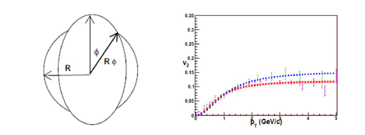
Figure 22: Left plot:Azimuthal dependence of R. R being the radius of the projected circle [158]. Right plot: Elliptic flow $v_{2}$ comparison with data and CSPM. The error bars in red and green are the results from Pb-Pb at $\sqrt{s_{NN}}$= 2.76 TeV and Au-Au at $\sqrt{s_{NN}}$= 200 GeV. The CSPM results are shown as dotted blue and red lines [159].

The transverse momentum dependence of $v_{2}$ computed using Eq. (130) for Pb-Pb at $\sqrt{s_{NN}}$ = 2.76 TeV and Au-Au at $\sqrt{s_{NN}}$ = 200 GeV for 10-20% centrality is shown in Fig. 22 (right plot). A good agreement is also obtained at all centralities and rapidities [158, 162].

The ridge structure was seen first at RHIC in Au-Au and Cu-Cu and later at LHC in Pb-Pb collisions. This structure has been also observed in proton-proton and proton-nucleus collisions at high multiplicity at LHC energies. This strong long range rapidity correlation collimated around azimuthal angles 0 and $\pi$ is one of the most interesting features of the experimental data, especially the structures seen in pp an pPb are a challenge for most of the models, in particular the hydrodynamics description.

In simple string models azimuthal dependence was not generated, so that the arising correlations were flat in $\phi$. In string percolation correlations can arise from the superposition of many events with different number and type of strings. In this way there appears long range correlations in rapidity as discussed earlier. However passing to the azimuthal dependence, if the emission from strings is isotropic, the correlations due to their distribution in different events will also be isotropic. Also in the central rapidity region the inclusive cross section are practically independent of rapidity. This generates a plateau in the $y-\phi$ distribution rather than a ridge, with only a narrow peak at small ${\it y}$ and $\phi$ due to short range correlations. This conclusion remains true if one averages the inclusive cross sections over all events with the resulting loss of azimuthal angle dependence. So the ridge can only be obtained on an event-by-event basis.

In string percolation the ridge arises due to fluctuations in both string distributions and impact parameter [161]. So it is important to study the averages relevant to the ridge formation. For a particular string configuration with a fixed azimuthal angle $\phi_{0}$ of the impact parameter, the single and double inclusive cross sections are

$$I^{c}(y,\phi)=A^{c}(y)+2\sum_{n=1}(B_{n}^{c}(y)\cos n(\phi-\phi_{0})+C_{m}^{c}\sin n(\phi-\phi_{0}))$$

$$=A^{c}(1+2\sum_{n=1}(b_{n}^{c}(y)\cos n(\phi)+c_{m}^{c}\sin n(\phi))$$ (131)

$$I^{c}(y_{1},\phi_{1},y_{2},\phi_{2})=\Big{[}A^{c}(y_{1})+2\sum_{n=1}(B_{n}^{c}(y_{1})\cos n(\phi_{1}-\phi_{0})+C_{n}^{c}\sin n(\phi_{1}-\phi_{0}))\Big{]}X$$

$$\Big{[}A^{c}(y_{2})+2\sum_{m=1}(B_{m}^{c}(y_{2})\cos m(\phi_{2}-\phi_{0})+C_{m}^{c}\sin m(\phi_{2}-\phi_{0}))\Big{]}.$$ (132)

One must average this expression over string distributions and directions of the impact parameter. The latter reduces to integration over with weight 1/2$\pi$. Doing first this integration and then averaging over string distribution one obtains the measured double inclusive cross section

$$I(y_{1},y_{2},\phi_{12})=<A(y_{1})A(y_{2})>+2\sum_{n}<W_{n}(y_{1},y_{2})>\cos n\phi_{12},$$ (133)

where $\phi_{12}=\phi_{1}-\phi_{2}$ and $W_{n}(y_{1},y_{2})=B_{n}(y_{1})B_{n}(y_{2})+C_{n}(y_{1})C_{n}(y_{2})$. Similar averaging of the single cross section eliminates all the azimuthal dependence $I(y_{1})$ = $<A(y_{1}>$. Thus the correlation function is

$$C(y_{1},y_{2},\phi_{12})=\frac{<A(y_{1})A(y_{2})>+2\sum_{n}<W_{n}(y_{1},y_{2})>\cos n\phi_{12}}{<A^{c}>^{2}}-1$$

$$=\frac{DA(y_{1},y_{2})}{<A(y_{1})><A(y_{2})>}+2\sum_{n=1}<w_{n}(y_{1},y_{2})>\cos n\phi_{12},$$ (134)

where $DA(y_{1},y_{2})$ and $w_{n}(y_{1},y_{2})$ are given by

$$DA(y_{1},y_{2})=<A(y_{1})A(y_{2})>-<A(y_{1})><A(y_{2})>,$$ (135)

$$w_{n}(y_{1},y_{2})=\frac{<W_{n}(y_{1},y_{2})>}{<A>^{2}}.$$ (136)

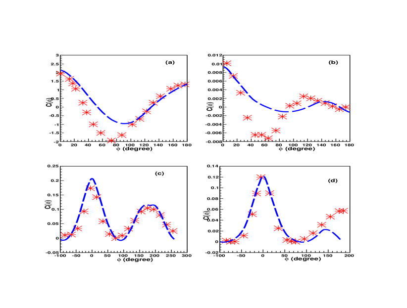
Figure 23: Correlation function $C(\phi)$ for (a). Au-Au at 200 GeV for 10% of the most central events along with experimental data (b). Pb-Pb at 2.76 TeV. (c). p-Pb collisions at 5.02 TeV for central collisions (d) pp collisions at 7 TeV [163].

The correlation contains two terms. The first is due to fluctuations in the total multiplicity and is independent of the angle. The ridge comes from the second term,which depends on the product of the initial coefficients $B_{n}$ and $C_{n}$ at different rapidities.

In the central rapidity region the distributions are practically independent of rapidity. This creates a plateau in rapidity with the angular dependence of correlations given by

$$C(\phi_{12})=\frac{DA}{<A>^{2}}+2\sum_{n=1}w_{n}\cos n\phi_{12}$$ (137)

with $DA$ = $<A^{2}>-<A>^{2}$, and $w_{n}=\frac{<B_{n}^{2}+C_{n}^{2}}{<A>^{2}}$. If one neglects fluctuations of the multiplicity at a given centrality and assumes $<A^{2}>$ = $<A>^{2}$ then one finds $w_{n}$ = $<v_{n}^{2}>$, the average of the individual flow coefficients squared. This should be compared with the normally defined flow coefficients which are obtained by averaging of individual coefficients themselves. If fluctuations both in $A$ and in $v_{n}$ are negligible one can take $<v_{n}^{2}>=<v_{n}>^{2}=v_{n}^{2}$ and thus find the ridge directly from the flow coefficients.

The general scheme of the calculations of $C(\phi_{12})$, Eq. (137), follows the Monte-Carlo code procedure used in the evaluations of the flow coefficients. In this case the color and tension of the clusters formed from $n$ original strings are taken to be $\sqrt{n}$ greater than the original strings without paying attention to the area of the formed cluster. This simplification is done to save computation time to do feasible the evaluations. In this way one computes the single and double inclusive cross-section and averaging them finds coefficients $v_{n},w_{n}$ and the correlation $C(\phi_{12})$.

Figures 23(a) and (b) show the results [163] of the correlation coefficient C($\phi$) for Au-Au at 200 GeV for 0-10% centrality and Pb-Pb at 2.76 TeV for the most central events together the experimental data [164, 27]. A good agreement is observed in the regions around $\phi=0$ and $\pi$. It worsens at intermediate azimuthal angles.

In pPb collisions we assume that the maximum number of strings attached to the nucleons of the target to be 18 at energies in the region 5-7 TeV, in accordance with the results on the multiplicity on pp collisions. The number of strings attached to the projectile proton will be $A^{1/3}$ times larger. The resulting $w_{n}$ and $C(\phi)$ are similar for energies 62.4, 200 GeV and 5.02 TeV. In Fig. 23(c) the correlation coefficient at 5.02 TeV for central collisions compared to the data [28] is shown. A very good agreement is observed.

String percolation describes $pp$ collisions in the same way as pA and AA collisions, therefore the same Monte-Carlo code procedure can be applied. From the multiplicity evaluations, it is known that the average number of formed strings at 62.4, 200 GeV and 7 TeV is 3, 4 and 9 respectively. For the distribution of hadronic matter in the proton a Gaussian of radius 0.8 fm is assumed. In Fig. 23(d) we show the correlation coefficient $C(\phi)$ for pp collisions at 7 TeV with triple multiplicity compared to the experimental data [29]. We again observe a very good agreement.

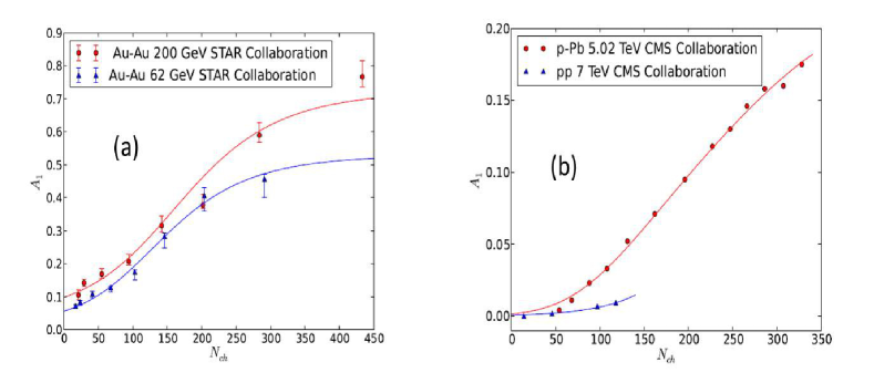
Figure 24: CSPM results on the strength of the near-side ridge for (a). Au-Au collisions at two RHIC energies. (b) pp collisions at 7 TeV and p-Pb collisions at 5.02 TeV [165].

Comparison with data at RHIC and LHC shows a good qualitative agreement in all cases. This agreement is also quantitative in cases of high multiplicity $pp$ and pPb collisions at 7 and 5.04 TeV respectively. The agreement with AA is reasonably good on the near side and on the away side but worse at intermediate angles. The reason for this probably has to do with simplifications in the simulations done to make calculations feasible. These simplifications eliminate part of the fluctuations and influence on the magnitude of higher harmonics. For instance, the multiplicity of a cluster was taken $\sqrt{n}$ instead of $\sqrt{nS_{n}/S_{1}}$ times the multiplicity of the original strings. Concerning the pseudorapidity dependence and the strength of the near side ridge structure together with the onset of it, the experimental data show an interesting behavior. The pp ridge structure only appears for charged multiplicity larger than 110 in pp collisions [29] and around 50 in pPb collisions [28]. On the other hand, the RHIC data on Au-Au indicate a change in the strength of the near side ridge structure at a given multiplicity [166]. All these facts can be naturally explained in string percolation [165]. In fact, the ridge structure in pp at high multiplicity was anticipated by string percolation [167].

It can be shown that the strength of the ridge structure $A_{1}$ defined as in  [166] is proportional to

$$\frac{dN}{dy}\frac{<n(n-1)>-<n>^{2}}{<n>^{2}},$$ (138)

which according to Eq. (117) of the previous section becomes $<N>/k$ where $N=N_{s}F(\xi)$ is the number of effective clusters and
$k=<N>/(1-exp(-\xi))^{3/2}$ the negative binomial parameter. Hence the strength of the near-side structure, $A_{1}$, is proportional to

$$A_{1}=\frac{<N>}{k}=C(1-\exp(-\xi))^{3/2}.$$ (139)

The factor $1-\exp(-\xi)$ stands for an homogeneous profile. In the case of more realistic profiles as Gaussian or Wood-Saxon we should use Eq.(15), thus

$$A_{1}=C\frac{1}{\Big{(}1+a\exp(-(\xi-\xi_{c}))/b\Big{)}^{3/2}},$$ (140)

where $C$ is a normalization constant which is different for each type of collision.

Comparison of the experimental data for the dependence of Au-Au at 62.4 and 200 GeV on the multiplicity [166] and pPb and pp at 5.04 and 7 TeV respectively [28] is shown in Figs. 24(a) and (b). In these figures the parameters $a$ and $\xi_{c}$ are kept fixed, with values 1.5 and 1.5 respectively (with these values one obtains the correct dependence of the fraction of the area covered by strings on the string density). The values of $b$ are 0.75 for Au-Au collisions and 0.35 for both pPb and pp collisions. We would expect $b\sim 1/R$, with $R$ the transverse dimension of the collision area, which is not far from the values found. Also a good agreement is found [165] for the behavior of the width in pseudorapidity of the ridge structure as a function of the multiplicity in Au-Au collisions at 62.4 and 200 GeV.

We conclude that string percolation is able to describe the ridge structures seen in pp high multiplicity, pPb and AA collisions. In this framework the ridge is obtained from the superposition of many events with different numbers and types of clusters of strings. In order to obtain anisotropy it is crucial to introduce quenching of the emitted partons in the strong color field inside the clusters of strings. In this way, it can be seen that the ridge structure in produced by an interplay of initial stage effects (formation of different clusters) and final state effects described by quenching.

3.4 Bose-Einstein correlations (BEC)

Studies of correlations between two identical particles have been very fruitful to determine the extension of the source of multiparticle production in collisions of two hadrons. This has been used extensively in heavy ion experiments at RHIC at LHC  [168, 169, 170, 171, 172, 173, 174]. These correlations provide information not only on the geometrical structure but also on the degree of coherence of the emitted particles. The correlation strength is characterized by a parameter $\lambda$, which can also be interpreted as a measure of chaoticity or the degree of coherence of the collision  [175, 176, 177]. In this interpretation $\lambda$ = 1 signals totally chaotic emission whereas $\lambda$ = 0 means radiation in a coherent way. However, this interpretation should be taken with caution. In fact, in $e^{+}-e^{-}$ annihilation, $\lambda$ is close to one at energies where there is no production of three or more jets and in the more complex pp collisions $\lambda$ decreases with increasing multiplicity. These observations would apparently suggests a systematic increase of the coherence from $e^{+}-e^{-}$ to pp collisions, which does not seem reasonable.

There are many difficulties in extracting the value of $\lambda$ from measurements (disentanglement from the Coulomb repulsion, corrections from long lived resonances, extrapolation to low $p_{t}$, corrections due to experimental transverse resolution). However, the existing measurements at ISR, SPS, RHIC and LHC give valuable information which should be understood. The experimental data on $\lambda$ have been obtained in different kinematic situations and also assuming different extrapolations, corrections and parametrizations, which makes rather difficult their comparison with theoretical models or even with different data. However some trends can be distinguished. First, for a not very large number of collisions, the data at SPS with p and Oxygen projectiles show a decrease of $\lambda$ with multiplicity [178, 179, 180]. As the number of collisions increases the behavior of $\lambda$ changes. It no longer decreases with multiplicity and even may increase. This is true at LHC where $\lambda$ reaches the values of 0.7-0.74. At SPS energies, the $\lambda$ values found are larger at forward than at central rapidity (Notice that the particle multiplicity is larger at central than in forward rapidity). This behavior can be naturally understood in the framework of percolation of strings [181, 182] .

The strings of the Lund type correspond to totally chaotic sources [183, 184], $\lambda$ = 1, and usually it is assumed that there is no BEC from a pair of particles emitted from different strings (a discussion on this assumption can be seen in [185]). Under these assumption one finds [186]

$$\lambda=\frac{n_{s}}{n_{tot}}$$ (141)

where $n_{s}$ is the mean number of identical particle pairs produced by fragmentation of the same string in a given rapidity and transverse momentum range and $n_{tot}$ is the total number of identical pairs produced in the same kinematic range. The number of pairs of identical particles produced by each cluster is

$$n_{s}=\frac{1}{2}\mu_{1}^{2}<\sum_{n=1}^{N_{s}}\frac{a_{n}nS_{n}}{S_{1}}>$$ (142)

and the total number of pair of identical particles produced is

$$n_{tot}=\frac{1}{2}\mu_{1}^{2}<\left(\sum_{n=1}^{N_{s}}\frac{a_{n}\sqrt{n}S_{n}}{S_{1}}\right)^{2}>$$ (143)

where $a_{n}$ is the number of clusters with $n$ strings, $\mu_{1}$ number of particles produced by a single string in the considered range. A Monte-Carlo simulation taking into account energy conservation was done at several energies and different projectiles and targets [181]. It was found that there is an approximate scaling in the string density, i.e. the chaoticity $\lambda$ only depends on it. In Fig. 25 values of $\lambda$ are shown as a function of the string density $\xi$. The details of the Monte-Carlo calculations together the SPS experimental results and the predictions for RHIC and LHC energies are shown in Ref. [181]. We observe a good agreement with the data in particular with the change of the behavior with multiplicity. Notice that the value of $\lambda$ = 0.7 predicted at LHC (last point in Fig. (25)) was confirmed by the LHC data [172, 173, 174].

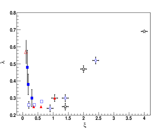
Figure 25: Dependence of $\lambda$ on $\xi$ for different nucleus-nucleus collisions with percolating strings [181].

The three body BEC have been also studied in the framework of percolation [182], predicting the strength of the genuine three particle Bose-Einstein correlations and obtaining a general agreement with experimental data  [174, 187, 188].

3.5 J/$\Psi$ Suppression

Melting of the J/$\Psi$ due to the Debye screening in a deconfined medium was one of the first proposed signatures of the existence of quark gluon plasma [8, 189]. Very early, at SPS energies, it was found that J/$\Psi$ was suppressed in S-U and O-U collisions [190, 191]. However this suppression was naturally explained by absorption of the pre-resonant cc state in the nucleus [192, 193]. From that time, many efforts have been devoted to disentangle the suppression due to nuclear effects from the actual melting in a deconfined medium. The RHIC and the LHC experimental data pointed out that, indeed, in addition to the nuclear effects there is a sequential suppression of J/$\Psi$ [194] combined with an enhancement due to a recombination mechanism [195] and to the existence of strong color fields above a certain matter density. On the other hand, ALICE collaboration [196] have shown that J/$\Psi$ production in pp high multiplicity events, normalized to the minimum bias, as a function of the multiplicity in the central rapidity region also normalized to the minimum bias increases linearly or even more rapidly at high multiplicity.

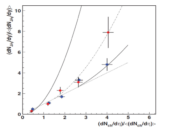
Figure 26: Our results for pp collisions in the central ($|y|<0.9$, dashed line) and forward (2.5 $<y<$4, dotted line) rapidity range, together with the experimental data for the central (circles) and forward (squares) rapidity regions from the ALICE collaboration [196]. The linear behavior(solid line) and our prediction for p-Pb collisions(solid line) at 7 TeV are also plotted [197].

In string percolation it is expected that above the critical percolation threshold the J/$\Psi$ or at least the $\Psi^{\prime}$s are suppressed. However, the string density reached at 7 TeV is much smaller than the percolation critical value even for high multiplicity events reached in the experiment. The behavior found by the ALICE collaboration can be naturally explained in the framework of string percolation [197]. In fact, assuming that, as in any hard process, the number of produced J/$\Psi$ is proportional to the number of collisions and thus is proportional to the number of strings $N_{s}$, we can write

$$\frac{n_{J/\Psi}}{<n_{J/\Psi}>}=\frac{N_{s}}{<N_{s}>}.$$ (144)

On the other hand we have

$$\frac{dN/dy}{<dN/dy>}=\frac{N_{s}F(\xi)}{<N_{s}>F(<\xi>)}.$$ (145)

From above equations we have

$$\frac{dN/dy}{<dN/dy>}=\left(\frac{n_{J/\Psi}}{<n_{J/\Psi}>}\right)^{1/2}\left(\frac{1-\exp(-\frac{n_{J/\Psi}<\xi>}{<n_{J/\Psi}>}}{1-\exp(-<\xi>)}\right)^{1/2}.$$ (146)

At low multiplicities where the number of strings $N_{s}$ is small, the above equation gives rise to the linear dependence

$$\frac{n_{J/\Psi}}{<n_{J/\Psi}>}=\frac{dN/dy}{<dN/dy>}.$$ (147)

On the other hand, at high multiplicities, the bracket on the right hand side of Eq. (146) can be approximated by $<\xi>^{-1/2}$. One obtains in this case

$$\frac{n_{J/\Psi}}{<n_{J/\Psi}>}=<\xi>\left(\frac{dN/dy}{<dN/dy>}\right)^{2}.$$ (148)

Thus the linear dependence obtained previously changes to quadratic when the high multiplicity events are in play. At much higher multiplicity, about 7-8 times minimum bias we predict a rapid suppression of this ratio. At 14 TeV the string density in pp increases by about 20% and thus at multiplicities of 5-7 times greater than at minimum bias there will be a suppression of J/$\Psi$ free of nuclear effects.

In Fig. (26) we show the results from Eq. (146) (dashed line) in the central rapidity region together the experimental data [196] (circles). Also the results for the forward region (dotted line) together with the data (squares) are shown. A very good agreement is observed. Note that in the forward direction there are less number of strings, producing less multiplicity and thus the departure of the linear behavior would be at higher multiplicities.

4 Thermodynamic and transport properties

A possible phase transition of strongly interacting matter from hadron to quark-gluon plasma state has received considerable interest in the past. What conditions are necessary in the pre-equilibrium stage to achieve deconfinement and perhaps subsequent Quark Gluon Plasma(QGP) formation ?

As discussed earlier in Section 2.2 the multiplicity $\mu$ and the mean transverse momentum squared $\langle p_{t}^{2}\rangle$ of the particles produced by a cluster of ${\it n}$ strings [198]

$$\mu_{n}=\sqrt{\frac{nS_{n}}{S_{1}}}\mu_{1};\hskip 14.22636pt\langle p_{t}^{2}\rangle=\sqrt{\frac{nS_{1}}{S_{n}}}{\langle p_{t}^{2}\rangle_{1}}$$ (149)

where $\mu_{1}$ and $\langle p_{t}^{2}\rangle_{1}$ are the mean multiplicity and $\langle p_{t}^{2}\rangle$ of particles produced from a single string with a transverse area $S_{1}=\pi r_{0}^{2}$. In the thermodynamic limit, one obtains an analytic expression [47, 198]

$$\langle\frac{nS_{1}}{S_{n}}\rangle=\frac{\xi}{1-e^{-\xi}}\equiv\frac{1}{F(\xi)^{2}};\hskip 14.22636ptF(\xi)=\sqrt{\frac{1-e^{-\xi}}{\xi}}$$ (150)

Here $\xi=\frac{N_{s}S_{1}}{S_{N}}$ is the percolation density parameter with $N_{S}$ and $S_{N}$ being the total number of strings and interaction area respectively. $F(\xi)$ is the color suppression factor and is related to $\mu_{n}$ and $\langle p_{t}^{2}\rangle_{n}$ through the relation $\mu_{n}=F(\xi)\mu_{0}$, $\langle p_{t}^{2}\rangle_{n}={\langle p_{t}^{2}\rangle_{1}}/F(\xi)$.

In this section thermodynamic and transport properties are discussed in the framework of clustering of color sources at RHIC and LHC energies. The thermodynamics of clustering can be addressed by extracting the temperature from the transverse momentum spectra of charged hadrons. In the model a local temperature can be introduced. In fact the tension of a cluster of strings fluctuates around its mean value because the chromoelectric field is not universal. Assuming a Gaussian form for these fluctuations a thermal spectrum is obtained with a temperature inversely proportional to $\sqrt{2F(\xi)}$. It is remarkable that for $\xi=1.2-1.5$ the corresponding temperature $T_{c}$ is not far from the critical temperature [199]. We extract the color suppression factor $F(\xi)$ using experimental data at RHIC energies. $F(\xi)$ and $\xi$ permit the determination of the initial temperature ${\it T}$ and the Bjorken initial energy density $\epsilon$. Energy density $\epsilon$ was found to be a linear function of $\xi$. As a result one can derive the equation of state and the transport coefficient shear viscosity over entropy density ratio as a function of the temperature. A good agreement between the model and lattice QCD results for energy density is obtained for $1<T/T_{c}<2$ [200]. Relativistic kinetic theory expression for shear viscosity has been used to obtain shear viscosity over entropy ratio $\eta/s$ at RHIC and LHC energies [201]. $\eta/s$ has a minimum at the temperature close to the critical one, rising slowly as the temperature increases. The data based values are compared with theoretical values for both a weakly coupled QGP (wQGP) and a strongly coupled QGP (sQGP). The dimensionless quantities, the trace anomaly $\Delta=(\epsilon-3p)/T^{4}$ and the inverse of $\eta/s$, have identical magnitudes for $0.5<T/T_{c}<6$ which describes the transition from wQGP to sQGP and then back to wQGP. This ’Ansatz’ provides an independent value for pressure at a given $\epsilon$ [202]. The sound velocity $C_{s}^{2}$ obtained using this pressure is in excellent agreement with the LQCD simulations [200].

4.1 Experimental determination of the color suppression factor $F(\xi)$

To evaluate the initial value of $\xi$ from data, a parameterization of p-p events at 200 GeV is used to compute the $p_{t}$ distribution [203]

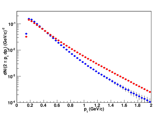
Figure 27: Charged particle $p_{t}$ spectrum from pp collisions (blue color) and Au-Au collisions at 200 GeV for 0-10% centrality [109].

$$dN_{c}/dp_{t}^{2}=a/(p_{0}+p_{t})^{\alpha},$$ (151)

where a, $p_{0}$, and $\alpha$ are parameters used to fit the data. Fig. 27 shows the normalized $p_{t}$ spectrum for pp collisions at $\sqrt{s}=$ 200 GeV. A fit to the data gives $p_{0}$ = 1.982 and $\alpha$ = 12.877. This parameterization is used for nucleus-nucleus collisions to take into account the interactions of the strings [203]

$$p_{0}\rightarrow p_{0}\left(\frac{\langle nS_{1}/S_{n}\rangle_{Au-Au}}{\langle nS_{1}/S_{n}\rangle_{pp}}\right)^{1/4},$$ (152)

where $S_{n}$ corresponds to the area occupied by the $n$ overlapping strings. The thermodynamic limit, i.e. letting $n$ and $S_{n}$ $\rightarrow\infty$ while keeping $\xi$ fixed, is used to evaluate

$$\langle\frac{nS_{1}}{S_{n}}\rangle=1/F^{2}(\xi)$$ (153)

$$dN_{c}/dp_{t}^{2}=\frac{a}{{(p_{0}{\sqrt{F(\xi_{pp})/F(\xi)}}+p_{t})}^{\alpha}}.$$ (154)

In pp collisions $\langle nS_{1}/S_{n}\rangle_{pp}$ $\sim$ 1 due to the low string overlap probability. The STAR analysis of charged hadrons for Au-Au collisions at $\sqrt{s_{NN}}$ = 200 and 62 GeV for $\xi$ is shown in Fig. 28 as a function of number of participants [203]. It is observed that for all centralities, except for the most peripheral one, $\sqrt{s_{NN}}$ = 200 GeV data lie above the critical percolation threshold $\xi_{c}$ = 1.2. The value of $\xi$ increases with increasing collision centrality, an expected indication of additional string overlap in more central collisions. For $\sqrt{s_{NN}}$ = 62.4 GeV, almost all centralities, except for the three most peripheral one lie above $\xi_{c}$.

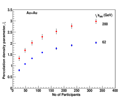
Figure 28: Percolation density parameter $\xi$ as a function of number of participants for Au-Au collisions at $\sqrt{s_{NN}}=$ 62 and 200 GeV [203].

Figure 29 shows a plot of $F(\xi)$ as a function of charged particle multiplicity per unit transverse area $\frac{dN_{c}}{d\eta}/S_{N}$ for Au-Au collisions at $\sqrt{s_{NN}}$ = 200 GeV for various centralities for the STAR data [109, 199]. The error on $F(\xi)$ is $\sim 3\%$. $F(\xi)$ decreases in going from peripheral to central collisions. The $\xi$ value is obtained using Eq. (150), which increases with the increase in centrality. The fit to the Au-Au points has the functional form

$$F(\xi)=\exp[-0.165-0.094\frac{dN_{c}}{d\eta}/S_{N}].$$ (155)

Recently, the ALICE experiment at LHC published the charged-particle multiplicity density data as a function of centrality in Pb-Pb collisions at $\sqrt{s_{NN}}$ = 2.76 TeV [115]. The STAR results for Au-Au collisions at $\sqrt{s_{NN}}$ = 200 GeV have been used to estimate F$(\xi)$ values for Pb-Pb collisions at different centralities using the fit function Eq. (155) for Au-Au.

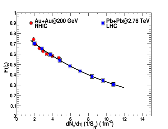
Figure 29: Color suppression factor $F(\xi)$ as a function of $\frac{dN_{c}}{d\eta}/S_{N}(fm^{-2})$. The solid red circles are for Au-Au collisions at 200 GeV (STAR data) [203]. The error is smaller than the size of the symbol. The line is fit to the STAR data. The solid blue squares are for Pb-Pb at 2.76 TeV [201].

4.2 Energy density

The QGP according to CSPM is born in local thermal equilibrium because the temperature is determined at the string level. After the initial temperature $T>T_{c}$ the CSPM perfect fluid may expand according to Bjorken boost invariant 1D hydrodynamics [7]

$$\varepsilon=\frac{3}{2}\frac{{\frac{dN_{c}}{dy}}\langle m_{t}\rangle}{S_{n}\tau_{pro}},$$ (156)

where $\varepsilon$ is the energy density, $S_{n}$ nuclear overlap area, and $\tau_{pro}$ the production time for a boson (gluon) [204].

The dynamics of massless particle production has been studied in QE2 quantum electrodynamics. QE2 can be scaled from electrodynamics to quantum chromodynamics using the ratio of the coupling constants [204]. The $\tau_{pro}$ for a boson (gluon) is [205]

$$\tau_{pro}=\frac{2.405\hbar}{\langle m_{t}\rangle}.$$ (157)

Above the critical temperature only massless particles are present in CSPM. To evaluate $\varepsilon$ we use the charged pion multiplicity $dN_{c}/{dy}$ at midrapidity and $S_{n}$ values from STAR for 0-10% central Au-Au collisions with $\sqrt{s_{NN}}=$200 GeV [199]. The factor 3/2 in Eq. (156) accounts for the neutral pions. The average transverse mass $\langle m_{t}\rangle$ is given by $\langle m_{t}\rangle=\sqrt{\langle p_{t}\rangle^{2}+m_{0}^{2}}$, where $\langle p_{t}\rangle$ is the transverse momentum of pion and $m_{0}$ being the mass of pion .

From the measured value of $\xi$ and $\varepsilon$, as shown in Fig. 30, it is found that $\varepsilon$ is proportional to $\xi$ for the range $1.2<\xi<2.88$, $\varepsilon=0.788$ $\xi$ (GeV/$fm^{3}$) [201]. The extrapolated value of $\varepsilon$ for central Pb-Pb collision at 2.76 TeV is 8.32 $GeV/fm^{3}$ as shown in Fig. 30.

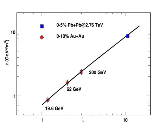
Figure 30: Energy density $\epsilon$ as a function of the percolation density parameter $\xi$. The extrapolated value for LHC energy is shown as blue square [201].

4.3 Temperature measurement and thermalization

The connection between $\xi$ and the temperature $T(\xi)$ involves the Schwinger mechanism (SM) for particle production. The Schwinger distribution for massless particles is expressed in terms of $p_{t}^{2}$ [205, 204]

$$dn/d{p_{t}^{2}}\sim\exp(-\pi p_{t}^{2}/x^{2})$$ (158)

where the average value of the string tension is $\langle x^{2}\rangle$. The tension of the macroscopic cluster fluctuates around its mean value because the chromo-electric field is not constant. The origin of the string fluctuation is related to the stochastic picture of the QCD vacuum. Since the average value of the color field strength must vanish, it can not be constant but changes randomly from point to point [103, 206]. Such fluctuations lead to a Gaussian distribution of the string tension

$$\frac{dn}{dp_{t}^{2}}\sim\sqrt{\frac{2}{<x^{2}>}}\int_{0}^{\infty}dx\exp(-\frac{x^{2}}{2<x^{2}>})\exp(-\pi\frac{p_{t}^{2}}{x^{2}})$$ (159)

which gives rise to thermal distribution [103]

$$\frac{dn}{dp_{t}^{2}}\sim\exp(-p_{t}\sqrt{\frac{2\pi}{\langle x^{2}\rangle}}),$$ (160)

with $\langle x^{2}\rangle$ = $\pi\langle p_{t}^{2}\rangle_{1}/F(\xi)$. The temperature is expressed as [104, 199]

$$T(\xi)={\sqrt{\frac{\langle p_{t}^{2}\rangle_{1}}{2F(\xi)}}}.$$ (161)

We will adopt the point of view that the experimentally determined chemical freeze-out temperature is a good measure of the phase transition temperature, $T_{c}$ [207]. The single string average transverse momentum ${\langle p_{t}^{2}\rangle_{1}}$ is calculated at $\xi_{c}$ = 1.2 with the universal chemical freeze-out temperature of 167.7 $\pm$ 2.6 MeV [208]. This gives $\sqrt{\langle{p_{t}^{2}}\rangle_{1}}$ = 207.2 $\pm$ 3.3 MeV which is close to $\simeq$ 200 MeV used previously in the calculation of percolation transition temperature [104].

Recently, it has been suggested that fast thermalization in heavy ion collisions can occur through the existence of an event horizon caused by a rapid deceleration of the colliding nuclei [209]. The thermalization in this case is due the Hawking-Unruh effect [210, 211].

It is well known that the black holes evaporates by quantum pair production and behave as if they have an effective temperature of

$$T_{H}=\frac{1}{8\pi GM},$$ (162)

where 1/4GM is the acceleration of gravity at the surface of a black hole of mass M. The rate of pair production in the gravitational background of the black hole can be evaluated by considering the tunneling through the event horizon. Unruh showed that a similar effect arises in a uniformly accelerated frame, where an observer detects the thermal radiation with the temperature T =a/2, where $a$ is the acceleration. Similarly, in hadronic interactions the probability to produce states of masses M due to the chromoelectric field E and color charge is given by the Schwinger mechanism

$$W_{M}\sim\exp(\frac{-\pi M^{2}}{gE})\sim\exp(-M/T),$$ (163)

which is similar to the Boltzmann weight in a heat bath with an effective temperature

$$T=\frac{a}{2\pi},a=\frac{2gE}{M}.$$ (164)

In CSPM the strong color field inside the large cluster produces de-acceleration of the primary $q\bar{q}$ pair which can be seen as a thermal temperature by means of Hawking-Unruh effect. This implies that the radiation temperature is determined by the transverse extension of the color flux tube/cluster in terms of the string tension [212, 213].

$$T={\sqrt{\frac{\sigma}{2\pi}}}$$ (165)

The string percolation density parameter $\xi$ which characterizes the percolation clusters measures the initial temperature of the system. Since this cluster covers most of the interaction area, this temperature becomes a global temperature determined by the string density. In this way at $\xi_{c}$ = 1.2 the connectivity percolation transition at $T(\xi_{c})$ models the thermal deconfinement transition.

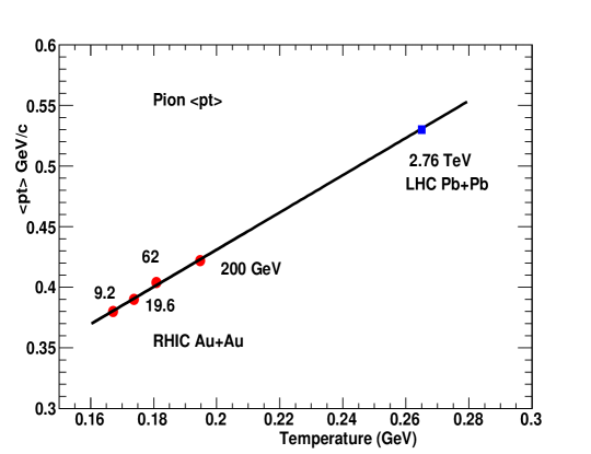
Figure 31: Average $<p_{t}>$ of pions as a function of temperature obtained using Eq. (161).

The temperature obtained using Eq. (161) was $\sim$ 193.6 MeV for Au-Au collisions at $\sqrt{s_{NN}}$ = 200 GeV in reasonable agreement with $T_{i}$ = 221 $\pm 19^{stat}\pm 19^{sys}$ from the enhanced direct photon experiment measured by the PHENIX Collaboration [16]. For Pb-Pb collisions at $\sqrt{s_{NN}}$ = 2.76 TeV the temperature is $\sim$ 262.2 MeV for 0-5$\%$ centrality, which is expected to be $\sim$ 35 $\%$ higher than the temperature from Au-Au collisions [199]. A recent summary of the results from Pb-Pb collisions at the LHC has mentioned that the initial temperature increases at least by 30 $\%$ as compared to the top RHIC energy [214]. The direct photon measurements from ALICE gives the temperature of $T_{i}$ = 304 $\pm 51$ [215]. The agreement with the measured temperaure shows that the temperature obtained using Eq. (161) can be termed as the initial temperature of the percolation cluster. For an ultrarelativistic ideal gas $\langle p_{t}\rangle\propto T$. Figure 31 shows a plot of $\langle p_{t}\rangle$ as a function of the temperature. When the transverse momentum is exponetially distributed with inverse slope T in a given event, $\langle p_{t}\rangle$ = 2 $T$ [216]. Using this relation one can predict the $\langle p_{t}\rangle$ for pions in Pb-Pb collisions at $\sqrt{s_{NN}}$ = 2.76 TeV. For 0-5 $\%$ the $\langle p_{t}\rangle$ = 0.53 GeV/c in agreement with the measured value of 0.517 $\pm$ 0.019 GeV/c [217]. Table I gives the CSPM values $\xi$, ${\it T}$, and $\varepsilon$ at $T/T_{c}$ = 0.88, 1, 1.16 and 1.57.

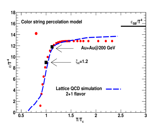
Figure 32: $\epsilon/T^{4}$ versus $T/T_{c}$ from CSPM (red circles) and Lattice QCD (blue dash line) for 2+1 flavor and p4 action [199].

Table 1: The percolation density parameter $\xi$, temperature ${\it T}$, $\tau{pro}$, and $\eta/s$ for meson gas [218], hadron to QGP transition in Au-Au collisions at 200 GeV and Pb-Pb at 2.76 TeV (estimated). Au-Au is for 0-10$\%$ and Pb-Pb is for 0-5$\%$ central events.

System	$\xi$	T (MeV)	$\eta/s$	$\tau_{pro}$ (fm)
Meson Gas	0.22	150.0	0.76
Hadron to QGP	1.2	167.7 $\pm 2.6$	0.240$\pm 0.012$
Au-Au	2.88$\pm 0.09$	193.6 $\pm 3.0$	0.204$\pm 0.020$	1.13
Pb-Pb	10.56$\pm 1.05$	262.2$\pm 13.0$	0.260$\pm 0.026$	0.89

4.4 Shear viscosity

The observation of the large elliptic flow at RHIC in non-central heavy ion collisions suggest that the matter created is a nearly perfect fluid with very low shear viscosity [15, 16, 17, 18]. Recently, attention has been focused on the shear viscosity to entropy density ratio $\eta/s$ as a measure of the fluidity [219, 220, 221, 222]. The observed temperature averaged $\eta/s$ based on viscous hydrodynamics analyses of RHIC data , are suggestive of a strongly coupled plasma [223, 224]. The effect of bulk viscosity is expected to be negligible. It has been conjectured, based on infinitely coupled super-symmetric Yang-Mills (SYM) gauge theory using the correspondence between Anti de-Sitter(AdS) space and conformal field theory (CFT), that the lower bound for $\eta/s$ is $1/4\pi$ and is the universal minimal $\eta/s$ even for QCD [19]. However, there are theories in which this lower bound can be violated [225].

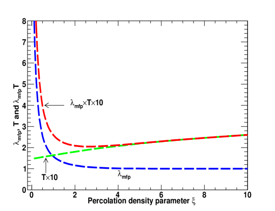
Figure 33: $\lambda_{mfp}$ in fm ( blue line), temperature in GeV scaled by a factor of 10(green line) and $\lambda_{mfp}\times$ scaled T in GeV fm (red line) as a function of $\xi$. The minimum in $\eta/s$ is due to the combination of $\lambda_{mfp}$ and T. Meson gas [218], RHIC and LHC points are also shown as solid black square [201].

The relativistic kinetic theory relation for the shear viscosity over entropy density ratio, $\eta/s$ is given by [223, 226]

$$\frac{\eta}{s}\simeq\frac{T\lambda_{mfp}}{5},$$ (166)

where T is the temperature and $\lambda_{mfp}$ is the mean free path. $\lambda_{mfp}\sim\frac{1}{(n\sigma_{tr})}$ where ${\it n}$ is the number density of an ideal gas of quarks and gluons and $\sigma_{tr}$ the transport cross section.

In CSPM the number density is given by the effective number of sources per unit volume [158, 227]

$$n=\frac{N_{sources}}{S_{N}L}.$$ (167)

L is the longitudinal extension of the string $\sim$ 1 ${\it fm}$ [104]. The area occupied by the strings is related to the percolation density parameter $\xi$ through the relation $(1-e^{-\xi})S_{N}$. Thus the effective no. of sources is given by the total area occupied by the strings divided by the area of an effective string $S_{1}F(\xi)$.

$$N_{sources}=\frac{(1-e^{-\xi})S_{N}}{S_{1}F(\xi)}.$$ (168)

In general $N_{sources}$ is smaller than the number of single strings. $N_{sources}$ equals the number of strings $N_{s}$ in the limit of $\xi$ = 0. The number density of sources from Eqs. (167) and (168) becomes

$$n=\frac{(1-e^{-\xi})}{S_{1}F(\xi)L}.$$ (169)

The transport cross section $\sigma_{tr}$ is the transverse area of the effective string $S_{1}F(\xi)$. Thus $\sigma_{tr}$ is directly proportional to $\frac{1}{T^{2}}$, which is in agreement with the estimated dependence of $\sigma_{tr}$ on the temperature [226, 228]. The mean free path is given by

$$\lambda_{mfp}={\frac{L}{(1-e^{-\xi})}}.$$ (170)

For large value of $\xi$ the $\lambda_{mfp}$ reaches a constant value. $\eta/s$ is obtained from $\xi$ and the temperature

$$\frac{\eta}{s}={\frac{TL}{5(1-e^{-\xi})}}$$ (171)

Below $\xi_{c}$, as the temperature increases, the string density increases and the area is filled rapidly and $\lambda_{mfp}$ and $\eta/s$ decrease sharply. Above $\xi_{c}$, more than 2/3 of the area are already covered by strings, and therefore the area is not filling as fast and the relatively small decrease of $\lambda_{mfp}$ is compensated by the rising of temperature, resulting in a smooth increase of $\eta/s$. The behavior of $\eta/s$ is dominated by the fractional area covered by strings. This is not surprising because $\eta/s$ is the ability to transport momenta at large distances and that has to do with the density of voids in the matter. Figure 33 shows a plot of $\lambda_{mfp}$, $T$ and $\lambda_{mfp}\times T$ as a function of $\xi$. Thus the product T($\xi$)$\times\lambda_{mfp}$ will have a minimum in $\eta/s$. It has been shown that $\eta/s$ has a minimum at the critical point for various substances for example helium, nitrogen and water [224]. Thus the measurement of $\eta/s$ as a function of temperature can locate the critical end point/crossover region in the QCD phase diagram $T\sim$ 175-185 MeV.

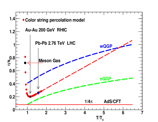
Figure 34: $\eta/s$ as a function of T/$T_{c}$. Au-Au at 200 GeV for 0-10$\%$ centrality is shown as solid black square. wQGP and sQGP values are shown as dotted blue and green lines respectively [223]. The red dotted line represents the extrapolation to higher temperatures from the CSPM [201]. The hadron gas value for $\eta/s$ $\sim$ 0.7 is shown as solid black circle at T/$T_{c}\sim$0.88 [218]. The red solid line is Ads/CFT limit [19].

Figure 34 shows a plot of $\eta/s$ as a function of T/$T_{c}$. The estimated value of $\eta/s$ for Pb-Pb is also shown in Fig. 34 at T/$T_{c}$ = 1.57. The lower bound shown in Fig. 34 is given by AdS/CFT [19]. The results from STAR and ALICE show that the $\eta/s$ value is 2.5 and 3.3 times the KSS bound [19]. Extrapolating the $\eta/s$ CSPM values it is clear that it will approach the weak coupling limit near $T/T_{c}$ $\sim$ 5.8 as the temperature is increased. The CSPM $\eta/s$ value for the hadron gas is in agreement with the calculated value using measured elastic cross sections for a gas of pions and kaons [218].

4.5 Jet quenching parameter

One of the outstanding observation made in central collisions of heavy ions is that the final state hadrons are strongly suppressed at large transverse momenta [229, 230]. This phenomena is referred as jet quenching, is understood to be caused by gluon radiation induced by multiple collisions of the leading parton while traversing the medium [231]. In QCD, the energy loss is expressed by the transport coefficient $\hat{q}$, which describes the rate at which medium transfers transverse momentum of the fast parton. An important question is whether different transport coefficients are related with each other. It was shown that two transport coefficients shear viscosity $\eta$ and jet quenching parameter $\hat{q}$ are related [231, 232].

$$\frac{\eta}{s}\approx{\frac{3}{2}\frac{T^{3}}{\hat{q}}}.$$ (172)

The relation associates a small ratio of $\eta/s$ to a large value of $\hat{q}$. A large amount of theoretical work has been done to extract the jet transport parameter from jet quenching at RHIC and LHC energies [229, 231, 232, 233]. The latest study by the JET Collaboration has extracted or calculated $\hat{q}$ from five different approaches to the parton energy loss in a dense medium. The evolution of bulk medium in the study was given by 2+1D or 3+1D hydrodynamic models with the initial temperatures of $T_{RHIC}^{Hydro}$ = 346 - 373 MeV and $T_{LHC}^{Hydro}$ = 447 - 486 MeV for most central Au-Au collisions at $\sqrt{s_{NN}}$ = 200 GeV and Pb-Pb collisions at $\sqrt{s_{NN}}$ = 2.76 TeV respectively.

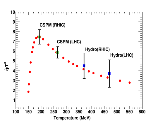
Figure 35: Scaled jet quenching parameter $\frac{\hat{q}}{T^{3}}$ as a function of the temperature. The values shown in solid blue squares (Hydro(RHIC) and Hydro(LHC) are given by Eq. (173). The CSPM values are shown in green solid squares CSPM(RHIC) and CSPM(LHC) for temperatures $\sim$193 and $\sim$262 MeV at RHIC and LHC energies respectively [201].

The variation of $\hat{q}$ values between different models can be considered as theoretical uncertainties. One therefore can extract its range of values at RHIC and LHC [229, 233]. The scaled $\hat{q}$ at the highest temperatures reached in the most central Au-Au collisions at RHIC and Pb-Pb collisions at LHC are

$$\frac{\hat{q}}{T^{3}}\approx\{^{4.5\pm 1.3\ at\ RHIC}_{3.7\pm 1.4\ at\ LHC}.$$ (173)

The corresponding absolute values for $\hat{q}$($GeV^{2}/fm$) for a 10 GeV quark jet are,

$$\hat{q}\approx\{^{1.2\pm 0.3\ }_{1.9\pm 0.7}{{}^{T=370MeV}_{T=470MeV}},$$ (174)

at an initial time $\tau_{0}=0.6fm/c$. The temperature dependence of scaled jet transport parameter $\frac{\hat{q}}{T^{3}}$ is shown in Fig. 35. The CSPM values for $\frac{\hat{q}}{T^{3}}$, using the relation given by Eq. (172), are shown in Fig. 35 (solid red circles). The CSPM values for RHIC and LHC energies are shown as solid green squares while the theoretical values are shown as blue squares. It is observed that CSPM values are in agreement with the JET Collaboration results.

The phase transition and $\hat{q}$ have been studied in the framework of dynamical holographic QCD model [234]. It is found that both $\hat{q}/T^{3}$ and trace anomaly $\Delta=(\varepsilon-3p)$ show a peak around the critical temperature $T_{c}$. This indicates that $\hat{q}$ can characterize the phase transition [234].

In the next section we show that in CSPM the inverse of $\eta/s$ is related to the trace anomaly.

4.6 Trace anomaly

The trace anomaly ($\Delta$) is the expectation value of the trace of the energy-momentum tensor, $\langle\Theta_{\mu}^{\mu}\rangle=(\varepsilon-3p)$, which measures the deviation from conformal behavior and thus identifies the interaction still present in the medium [235]. We find that the reciprocal of $\eta/s$ is in quantitative agreement with $(\varepsilon-3p)/T^{4}$ over a wide range of temperatures [202, 236]. This result is shown in Fig. 36. The minimum in $\eta/s\sim 0.20$ determines the peak of the interaction measure $\sim$ 5 in agreement with the recent HotQCD values [200]. This happens at the critical temperature of $T_{c}\sim 175$ MeV. Figure 36 also shows the results from Wuppertal Collaboration [237]. The maximum in $\Delta$ corresponds to the minimum in $\eta/s$. Both $\Delta$ and $\eta/s$ describe the transition from a strongly coupled QGP to a weakly coupled QGP.

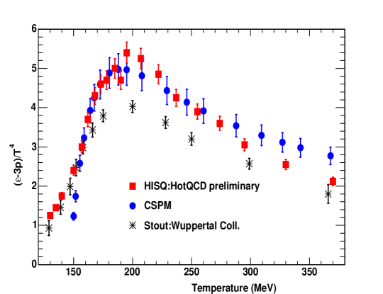
Figure 36: The trace anomaly $\Delta=(\varepsilon-3p)/T^{4}$ vs temperature [200]. Red solid squares are from HotQCD Collaboration [200]. Black stars are from Wuppertal Collaboration [237].

4.7 Equation of State: Sound velocity

We use CSPM coupled to a 1D Bjorken expansion. The input parameters are the initial temperature T, the initial energy density $\varepsilon$, and the trace anomaly $\Delta$ are determined by data. The Bjorken 1D expansion gives the sound velocity

$$\frac{1}{T}\frac{dT}{d\tau}=-C_{s}^{2}/\tau$$ (175)

$$\frac{dT}{d\tau}=\frac{dT}{d\varepsilon}\frac{d\varepsilon}{d\tau}$$ (176)

$$\frac{d\varepsilon}{d\tau}=-Ts/\tau,$$ (177)

where $\varepsilon$ is the energy density, s the entropy density, $\tau$ the proper time, and $C_{s}$ the sound velocity. Since $s=(\varepsilon+P)/T$ and $P=(\varepsilon-\Delta T^{4})/3$ one gets

$$\frac{dT}{d\varepsilon}s=C_{s}^{2}.$$ (178)

From above equations $C_{s}^{2}$ can be expressed in terms of $\xi$

$$C_{s}^{2}=(-0.33)\left(\frac{\xi e^{-\xi}}{1-e^{-\xi}}-1\right)+\\ 0.0191(\Delta/3)\left(\frac{\xi e^{-\xi}}{({1-e^{-\xi}})^{2}}-\frac{1}{1-e^{-\xi}}\right)$$ (179)

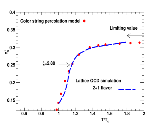
Figure 37: The speed of sound from CSPM versus $T/T_{c}^{CSPM}$(red circles) and Lattice QCD-p4 speed of sound versus $T/T_{c}^{LQCD}$(blue dash line) [238].

Since there is no direct way to obtain pressure in CSPM, we have made the assumption that $\Delta=(\varepsilon-3P)\approx 1/(\eta/s)$ . Fig. 37 shows a plot of $C_{s}^{2}$ as a function of $T/T_{c}$. It is observed that the CSPM results are in very good agreement with the lattice calculations [238]. This suggest that the $\Delta$ can be approximated to $1/(\eta/s)$.

5 Summary

The string percolation gives a successfully description of most of the experimental data in the soft region, including rapidity distributions, probability distributions of multiplicities and transverse momentum, strength of the B-E correlations, elliptic flow and ridge structures. The clustering of color sources has a clear physical basis, although is not derived directly from QCD, but has its most fundamental features. The non-Abelian character is reflected in the coherence sum of the color fields which as a consequence gives rise to an enhancement of the transverse momentum and a relative multiplicity suppression. The confinement is reflected in the small transverse size of the strings as well as in the length of the transverse correlations. The scaling observed in the transverse momentum distribution is a consequence of the invariance of the probability distributions under the transformations of the size of the clusters of strings.

The interpretation of data using string CSPM describes the equation of state close to the critical temperature and also obtains a reasonable dependence on the temperature of the shear viscosity over entropy density ratio. Thermodynamical results are also in agreement with the lattice QCD calculations. The percolation critical transition is known to represent a continuous phase transition. In central Au-Au collisions at $\sqrt{s_{NN}}=$ 200 GeV the QCD to hadron phase transition for baryon density $\mu_{B}\sim$ 0 is believed to be a cross-over transition which does not have a latent heat. The CSPM EOS correctly describes the QCD to hadron cross-over transition and provides an answer to the question of the origin of universal temperature observed in A-A, p-p and $e^{+}e^{-}$ collisions. The percolation framework provides us with a microscopic picture which predicts the early thermalization required for hydrodynamical calculations.

The minimum in $\eta/s$ can be studied as a function of the beam energy at RHIC that could locate the critical point/crossover in the QCD phase diagram seen in substances like helium, nitrogen and water. The accurate determination of $\eta/s$ is also important for the evaluation of another transport coefficient, the jet quenching parameter $\hat{q}$.

There are many similarities between string percolation and the Glasma of the color glass condensate, in formal aspects and also in phenomenological applications. In this way string percolation can be regarded as a complementary view of CGC of the initial stage of a high hadronic collision.

Acknowledgements

This research was supported by the Office of Nuclear Physics within the U.S. Department of Energy Office of Science under Grant No. DE-FG02-88ER40412. M.A.B. appreciates the support of S.Petersburg State University grant 11.38.197.2014 . J.D.D. thanks the support of the FCT/Portugal project PPCDT/FIS/575682004. C.P. was supported by the project FPA2011-022776 of MICINN the Spanish Consolider Ingenio 2010 program CPAN and Conselleria Education Xunta de Galicia.

References

- [1] I. Y. Pomeranchuk, Quantum chromodynamics and the pomeron, Sov. Phys. JETP 3 (1956) 306.
- [2] T. D. Lee, G. C. Wick, Vacuum stability and vacuum excitation in a spin-0 field theory, Phys. Rev. D 9 (1974) 2291.
- [3] J. C. Collins, M. J. Perry, Super dense matter: Neutrons or asymptotically free quarks ?, Phys. Rev. Lett. 34 (1975) 1353.
- [4] N. Cabibbo, G. Parisi, Exponential hadronic spectrum and quark liberation, Phys. Lett. B 59 (1975) 67.
- [5] E. V. Shuryak, Quark-gluon plasma and production of leptons, photons and psions, Phys. Lett. B 78 (1978) 150.
- [6] J. Hofmann, H. Stocker, W. Scheid, W. Greiner, Bear Montain Workshop, 1974.
- [7] J. D. Bjorken, Highly relativistic nucleus-nucleus collisions: The central rapidity region, Phys. Rev. D 27 (1983) 140.
- [8] T. Matsui, H. Satz, J/ suppression by quark-gluon plasma formation, Phys. Lett. B 178 (1986) 416.
- [9] J. D. Bjorken, Energy loss of energetic partons in quark-gluon plasma: Possible extinction of high jets in hadron-hadron collisions, Fermi-Lab. Pub-82/59-THY, 1982.
- [10] M. Gyulassy, X. N. Wang, Multiple collisions and induced gluon bremsstrahlung in QCD, Nucl. Phys. B 420 (1994) 583.
- [11] G. Baym, Confinement of quarks in nuclear matter, Physica A 96 (1979) 131.
- [12] T. Celik, F. Karsch, H. Satz, A percolation approach to strongly interacting matter, Phys. Lett. B 97 (1980) 128.
- [13] B. Schwarzschild, Mapping the interstellar cloud we live in, Physics Today 53 (2000) 20.
- [14] M. Gyulassy, L. McLerran, New forms of QCD matter discovered at RHIC, Nucl. Phys. A 750 (2005) 30.
- [15] J. Adams et al. (STAR Collaboration), Experimental and theoretical challenges in the search for the quark-gluon plasma: The STAR Collaboration’s critical assessment of the evidence from RHIC collisions, Nucl. Phys. A 757 (2005) 102.
- [16] K. Adcox et al., Formation of dense partonic matter in relativistic nucleus-nucleus collisions at RHIC: Experimental evaluation by the PHENIX Collaboration, Nucl. Phys. A 757 (2005) 184.
- [17] B. B. Back et al. (PHOBOS Collaboration), The PHOBOS perspective on discoveries at RHIC, Nucl. Phys. A 757 (2005) 28.
- [18] I. Arsene et al. (BRAHMS Collaboration), Quark-gluon plasma and color glass condensate at RHIC ? The perspective from the BRAHMS experiment, Nucl. Phys. A 757 (2005) 1.
- [19] P. K. Kovtun, D. T. Son, A. O. Starinets, Viscosity in strongly interacting quantum field theories from black hole physics, Phys. Rev. Lett. 94 (2005) 111601.
- [20] K. Aamodt et al. (ALICE Collaboration), Elliptic flow of charged particles in Pb-Pb collisions at = 2.76 TeV, Phys. Rev. Lett. 105 (2010) 252302.
- [21] S. Chatrchyan et al. (CMS Collaboration), Measurement of the elliptic anisotropy of charged particles produced in Pb-Pb collisions at = 2.76 TeV, Phys. Rev. C 87 (2013) 014902.
- [22] G. Aad et al. (ATLAS Collaboration), Measurement of the pseudorapidity and transverse momentum dependence of the elliptic flow of charged particles in lead-lead collisions at = 2.76 TeV with the ATLAS detector, Phys. Lett. B 707 (2012) 330.
- [23] K. Aamodt et al. (ALICE Collaboration), Higher harmonic anisotropic flow measurements of charged particles in Pb-Pb collisions at = 2.76 TeV, Phys. Rev. Lett. 107 (2011) 032301.
- [24] S. Chatrchyan et al. (CMS Collaboration), Studies of dihadron correlations in ultra-central Pb-Pb collisions at = 2.76 TeV, JHEP 02 (2014) 088.
- [25] A. Adare et al. (PHENIX Collaboration), Dihadron azimuthal correlations in Au-Au collisions at = 200 GeV, Phys. Rev. C 78 (2008) 014901.
- [26] M. M. Aggarwal et al. (STAR Collaboration), Azimuthal di-hadron correlations in d+Au and Au-Au collisions at = 200 GeV measured at the STAR detector, Phys. Rev. C 82 (2010) 024912.
- [27] B. Abelev et al. (ALICE Collaboration), Long-range angular correlations on the near and away side in p-Pb collisions at = 5.02 TeV, Phys. Lett. B 719 (2013) 29.
- [28] S. Chatrchyan et al. (CMS Collaboration), Observation of long-range, near-side angular correlations in pPb collisions at the LHC, Phys. Lett. B 718 (2013) 795.
- [29] S. Chatrchyan et al. (CMS Collaboration), Multiplicity and transverse momentum dependence of two- and four-particle correlations in pPb and Pb-Pb collisions, Phys. Lett. B 724 (2013) 213.
- [30] V.Khachatryan et al. (CMS Collaboration), Observation of long range, near-side angular correlations in proton-proton collisions at the LHC, JHEP 09 (2010) 091.
- [31] S. Chatrchyan et al. (CMS Collaboration), Observation of sequential suppression in Pb-Pb collisions, Phys. Rev. Lett. 109 (2012) 222301.
- [32] B. Abelev et al. (ALICE Collaboration), Centrality, rapidity and transverse momentum dependence of suppression in Pb-Pb collisions at = 2.76 TeV, Phys. Lett. B 734 (2014) 314.
- [33] G. Aad et al. (ATLAS Collaboration), Measurement of the centrality dependence of yields and observation of Z production in lead-lead collisions with the ATLAS detector at the LHC, Phys. Lett. B 697 (2011) 294.
- [34] S. Chatrchyan et al. (CMS Collaboration), Study of high- charged particle suppression in Pb-Pb compared to pp collisions at = 2.76 TeV, Eur. Phys. J C 72 (2012) 1945.
- [35] L. McLerran, R. Venugopalan, Computing quark and gluon distribution functions for very large nuclei, Phys. Rev. D 49 (1994) 2233.
- [36] L. McLerran, R. Venugopalan, Gluon distribution functions for very large nuclei at small transverse momentum, Phys. Rev. D 49 (1994) 3352.
- [37] L. McLerran, R. Venugopalan, Green’s function in the color field of a large nucleus, Phys. Rev. D 50 (1995) 2225.
- [38] E. Iancu, A. Leonidov, L. McLerran, Nonlinear gluon evolution in the color glass condensate, Nucl. Phys. A 692 (2001) 583.
- [39] E. G. Ferreiro, E. Iancu, K. Itakura, L. McLerran, Froissart bound from gluon saturation, Nucl. Phys. A 710 (2002) 373.
- [40] L. V. Gribov, E. M. Levin, M. G. Ryskin, Semihard processes in QCD, Phys. Rep. 100 (1983) 1.
- [41] D. Kharzeev, M. Nardi, Hadron production in nuclear collisions at RHIC and high-density QCD, Phys. Lett. B 507 (2001) 121.
- [42] D. Kharzeev, E. Levin, Manifestations of high density QCD in the first RHIC data, Phys. Lett. B 523 (2001) 79.
- [43] T. Lappi, L. McLerran, Some features of the glasma, Nucl. Phys. A 772 (2006) 200.
- [44] N. Armesto, M. A. Braun, E. G. Ferreiro, C. Pajares, Percolation approach to Quark-Gluon Plasma and suppression, Phys. Rev. Lett. 77 (1996) 3736.
- [45] M. Nardi, H. Satz, String clustering and suppression in nuclear collisions, Phys. Lett. B 442 (1998) 14.
- [46] M. A. Braun, C. Pajares, J. Ranft, Fusion of strings vs. percolation and the transition to the Quark-Gluon Plasma, Int. J. Mod. Phys. A 14 (17) (1999) 2689.
- [47] M. A. Braun, C. Pajares, Implications of color-string percolation on multiplicities, correlations, and the transverse momentum, Eur. Phys. J. C 16 (2000) 349.
- [48] M. A. Braun, C. Pajares, Transverse momentum distributions and their forward-backward correlations in the percolating color string approach, Phys. Rev. Lett. 85 (2000) 4864.
- [49] M. B. Isichenko, Percolation, statistical topography, and transport in random media, Rev. Mod. Phys. 64 (1992) 961.
- [50] J. Dias de Deus, C. Pajares, String percolation and the Glasma, Phys. Lett. B 695 (2011) 211.
- [51] H. Satz, Extreme states of matter in strong interaction physics, Lecture Notes in Physics 841, Springer 2012.
- [52] N. F. Mott, The basis of the electron theory of metals, with special reference to the transition metals, Proc. Phys. Soc. A 62 (1949) 416.
- [53] A. Andronic et al., Hadron production in ultra-relativistic nuclear collisions: Quarkyonic matter and a triple point in the phase diagram of QCD, Nucl. Phys. A 837 (2010) 85.
- [54] H. Satz, Color screening in SU(N) gauge theory at finite temperature, Nucl. Phys. A 418 (1984) 447.
- [55] P. Castorina, R. V. Gavai, H. Satz, The QCD phase structure at high density, Eur. Phys. J. C 69 (2010) 169.
- [56] K. Rajagopal, F. Wilczek, The condensed matter physics of QCD, hep-ph/0011333.
- [57] M. Alford, A. Schmitt, K. Rajagopal, T. Schafer, Color superconductivity in dense dark matter, Rev. Mod. Phys. 80 (2008) 1455.
- [58] L. McLerran, K. Redlich, C. Sasaki, Quarkyonic matter and chiral symmetry breaking, Nucl. Phys. A 824 (2009) 86.
- [59] S. Borsanyi et al., Is there still any mystery in lattice QCD ? Results with physical masses in the continuum limit III, JHEP 09 (2010) 073.
- [60] A. Bazavov et al. (HotQCD Collaboration), Chiral and deconfinement aspects of the QCD transition, Phys. Rev. D 85 (2012) 054503.
- [61] P. Petreczky, Lattice QCD at non-zero temperature, J. Phys. G: Nucl. Part. Phys. 39 (2012) 093002.
- [62] D. Stauffer, A. Aharony, Introduction to percolation theory CRC Press, 1994.
- [63] A. Rodrigues, R.Ugoccioni, J. Dias de Deus, Percolation approach to phase transitions in high energy nuclear collisions, Phys. Lett. B 458 (1999) 402.
- [64] G. R. Grimmett, Percolation, Springer-Verlag, New York 2nd Ed. XII (1999) 447.
- [65] P. Castorina, K. Redlich, H. Satz, Phase diagram of hadronic matter, Eur. Phys. J. C 59 (2009) 67.
- [66] C. Gattringer, Coherent center domains in SU(3) gluodynamics and their percolation at , Phys. Lett. B 690 (2010) 179.
- [67] J. Danzer, C. Gattringer, S. Borsanyi, Z. Fodor, Center clusters and their percolation properties in lattice QCD, PoS Lattice2010 (2010) 176.
- [68] M. Beccaria, A. Moro, Cluster percolation and chiral phase transition, Phys. Rev. D 66 (2002) 037502.
- [69] M. Asakawa, S. A. Bass, B. Muller, Center domains and their phenomenological consequences, Phys. Rev. Lett. 110 (2013) 202301.
- [70] A. Capella, U. Sukhatme, C.-I. Tan, J. Tran Thanh Van, Dual Parton Model, Phys. Rep. 236 (1994) 225.
- [71] A. Capella, U. Sukhatme, C.-I. Tan, J. Tran Thanh Van, Jets in small- hadronic collisions, universality of quark fragmentation, and rising rapidity plateaus, Phys. Lett. B 81 (1979) 68.
- [72] K. Werner, Strings, pomerons and the VENUS model of hadronic interactions at ultrarelativistic energies, Phys. Rep. 232 (1993) 87.
- [73] A. B. Kaidalov, K. A. Ter-Martirosyan, Pomeron as quark-gluon strings and multiple hadron production at SPS-collider energies, Phys. Lett. B 117 (1982) 247.
- [74] K. Werner et al., Gribov-Regge theory, partons, remnants, strings-and the EPOS model for hadronic interactions, Nucl. Phys. B Proc. suppl. 196 (2009) 36.
- [75] F. W. Bopp, J. Ranft, R. Engel, S. Roesler, Learning from RHIC data with DPMJET-III, Acta. Phys. Polon. B 35 (2004) 303.
- [76] X. N. Wang, M. Gyulassy, HIJING: A Monte Carlo model for multiple jet production in pp, pA and AA collisions, Phys. Rev. D 44 (1991) 3501.
- [77] T. Sjostrand, S. Mrenna, P. Skands, A brief introduction to PYTHIA 8.1, Comput. Phys. Commun. 178 (2008) 852.
- [78] Zi-Wei Lin, C. M. Ko, Bao-An Li, B. Zhang, S. Pal, Multiphase transport model for relativistic heavy ion collisions, Phys. Rev. C 72 (2005) 064901.
- [79] M. Bleicher et al., Relativistic hadron-hadron collisions in the ultra-relativistic quantum molecular dynamics model, J. Phys. G 25 (1999) 1859.
- [80] A. Abramovski, V. N. Gribov, O. Kancheli, Character of inclusive spectra and fluctuations produced in inelastic processes by Multi-Pomeron exchange, Sov. J. Nucl. Phys. 18 (1974) 308.
- [81] A. Capella, A. Staar, J. Tran Thanh Van, Koba-Nielsen-Olesen-scaling violations in the dual parton model, Phys. Rev. D 32 (1985) 2933.
- [82] A. Capella, A. Krzywicki, Unitarity corrections to short range-order: Long-range rapidity correlations, Phys. Rev. D 18 (1978) 4120.
- [83] T. T. Chou, C. N. Yang, A unified physical picture: Narrow Poisson-like distribution for two -jet events and wide approximate KNO distribution for hadron-hadron collisions, Phys. Lett. B 167 (1986) 453.
- [84] V. Vechernin, Forward-backward multiplicity correlations in windows separated in azimuth and rapidity, arXiv:1210.7588.
- [85] A. Capella, C. Pajares, A. V. Ramallo, High energy nucleus-nucleus collisions in the dual parton model, Nucl. Phys. B 241 (1984) 75.
- [86] A. Bialas, B. Bleszynski, W. Czyz, Multiplicity distributions in nucleus-nucleus collisions at high energies, Nucl. Phys. B 111 (1976) 461.
- [87] C. Pajares, A. V. Ramallo, Effects of the multiple-scattering structure in the propagation of hadronic properties in nucleus-nucleus collisions, Phys. Rev. D 31 (1985) 2800.
- [88] K. G. Boreskov, A. B. Kaidalov, Nucleus-nucleus scattering in the Glauber approach, Sov. J. Nucl. Phys. 48 (1988) 367.
- [89] B. Andersson, G. Gustafson, B. Nilsson-Almqvist, A model for low- hadronic reactions with generalizations to hadron-nucleus and nucleus-nucleus collisions, Nucl. Phys. B 281 (1987) 289.
- [90] M. Gyulassy, CERN preprint CERN -TH 4794, 1987.
- [91] H. Sorge, H. Stocker, W. Greiner, Relativistic quantum molecular approach to nuclear collisions at ultrarelativistic energies, Nucl. Phys. A 498 (1989) 567c.
- [92] T. S. Biro, H. B. Nielsen, J. Knoll, Color rope model for extreme relativistic heavy ion collisions, Nucl. Phys. B 245 (1984) 449.
- [93] M. A. Braun, C. Pajares, Particle production in nuclear collisions and string interactions, Phys. Lett.B 287 (1992) 154.
- [94] N. S. Amelin, M. A. Braun, C. Pajares, Multiple production in the Monte Carlo string fusion model, Phys. Lett. B 306 (1993) 312.
- [95] N. S. Amelin, M. A. Braun, C. Pajares, String fusion and particle production at high energies: Monte Carlo string fusion model, Z fur Physik C 63 (1994) 507.
- [96] A. Bialas, W. Czyz, Conversion of color field into matter in the central region of high-energy heavy ion collisions, Nucl. Phys. B 267 (1986) 242.
- [97] D. Stauffer, Scaling theory of percolation clusters, Phys. Rep. 54 (1979) 1.
- [98] R. Baier, Yu L. Dokshitzer, A. H. Mueller, S. Peigne, D. Schiff, Radiative energy loss of high energy quarks and gluons in the finite-volume quark-gluon plasma, Nucl. Phys. B 483 (1997) 291.
- [99] R. Baier, Yu L. Dokshitzer, A. H. Mueller, S. Peigne, D. Schiff, Radiative energy loss and broadening of high energy partons in nuclei, Nucl. Phys. B 484 (1997) 265.
- [100] A. I. Nikishov, V. I. Ritus, Interaction of electrons and photons with a very strong magnetic field, Sov. Phys. Uspekhi 13 (1970) 303.
- [101] A. Mikhailov, Nonlinear waves in AdS/CFT, hep-th/0305196.
- [102] A. I. Nikishov, Barrier scattering in field theory removal of Klein paradox, Nucl. Phys. B 21 (1970) 346.
- [103] A. Bialas, Fluctuations of the string tension and transverse mass distribution, Phys. Lett. B 466 (1999) 301.
- [104] J. Dias de Deus, C. Pajares, Percolation of color sources and critical temperature, Phys. Lett. B 642 (2006) 455.
- [105] N. Van Eijndhoven et al., The ALICE event generator pool, ALICE/GEN 95-32, Internal note.
- [106] I. Bautista, J. G. Milhano, C.Pajares, J. Dias de Deus, Multiplicity in pp and AA collisions: The same power law from energy-momentum constrains in string production, Phys. Lett. B 715 (2012) 230.
- [107] C. Albajar et al. (UA1 Collaboration), A study of the general characteristics of proton-antiproton collisions at = 0.2 to 0.9 TeV, Nucl. Phys. B 335 (1990) 261.
- [108] G. J. Alner et al. (UA5 Collaboration), UA5: A general study of proton-antiproton physics at =546 GeV, Phys. Rep. 154 (1987) 247.
- [109] B. I. Abelev et al. (STAR Collaboration), Systematic measurements of identified particle spectra in pp, d+Au and Au-Au collisions with the STAR detector, Phys. Rev. C 79 (2009) 34909.
- [110] F. Abe et al. (CDF Collaboration), Pseudorapidity distributions of charged particles produced in p interactions at = 630 and 1800 GeV, Phys. Rev. D 41 (1990) 2330.
- [111] K. Aamodt et al. (ALICE Collaboration), Charged-particle multiplicity measurements in proton-proton collisions at = 0.9 and 2.36 TeV with ALICE at LHC, Eur. Phys. J. C 68 (2010) 89.
- [112] V. Khachatryan et al. (CMS Collaboration), Transverse-momentum and pseudorapidiy distributions of charged hadrons in pp collisions at = 0.9 and 2.36 TeV, JHEP 02 (2010) 041.
- [113] V. Khachatryan et al. (CMS Collaboration), Transverse-momentum and pseudorapidity distributions of charged hadrons in pp collisions at = 7 TeV, Phys. Rev. Lett. 105 (2010) 022002.
- [114] B. Alver et al., Charged-particle multiplicity and pseudorapidity distributions measured with the PHOBOS detector in Au-Au, Cu-Cu, d+Au, and p+p collisions at ultrarelativistic energies, Phys. Rev. C 83 (2011) 024913.
- [115] K. Aamodt et al. (ALICE Collaboration), Centrality dependence of charged particle multiplicity density at midrapidity in Pb-Pb collisions at = 2.76 TeV, Phys. Rev. Lett. 106 (2011) 032301.
- [116] J. Dias de Deus, J. G. Milhano, Energy conservation and scaling violations in particle production, Phys. Lett. B 662 (2008) 129.
- [117] P. Brogueira, J. Dias de Deus, C. Pajares, Limiting fragmentation in heavy-ion collisions and percolation of strings, Phys. Rev. C 75 (2007) 054908.
- [118] I. Bautista, C. Pajares, J. Dias de Deus, Evolution of particle density in high-energy pp collisions, Nucl. Phys. A 882 (2012) 44.
- [119] I. Bautista, C. Pajares, J. G. Milhano, J. Dias de Deus, Rapidity dependence of particle densities in pp and AA collisions, Phys. Rev. C 86 (2012) 034909.
- [120] G. Antchev et al. (TOTEM Collaboration), Measurements of the forward charged-particle pseudorapidity density in pp collisions at = 7 TeV, Eur. Phys. Lett 98 (2012) 31002.
- [121] B. Alver et al. (PHOBOS Collaboration), System size, energy, and centrality dependence of pseudorapidity distributions of charged particles in relativistic heavy ion collisions, Phys. Rev. Lett. 102 (2012) 142301.
- [122] B. B. Back et al. (PHOBOS Collaboration), Significance of the fragmentation region in ultrarelativistic heavy ion collisions, Phys. Rev. Lett. 91 (2003) 052303.
- [123] S. Chatrchyan et al. (CMS Collaboration), Dependence on pseudorapidity and on centrality of charged hadron production in Pb-Pb collisions at = 2.76 TeV, JHEP 08 (2011) 141.
- [124] C. Merino, C. Pajares, Y. M. Shabelski, Production secondaries in high-energy d+Au collisions, Eur. Phys J. C 59 (2009) 691.
- [125] E. Levin, A. H. Rezaeian, Gluon saturation and energy dependence of hadron multiplicity in pp and AA collisions at the LHC, Phys. Rev. D 83 (2001) 114001.
- [126] T. Lappi, Energy dependence of the saturation scale and the charged multiplicity in pp and AA collisions., Eur. Phys. J. C 71 (2011) 1699.
- [127] J. Dias de Deus, E. G. Ferreiro, C. Pajares, R. Ugoccioni, Universality of the transverse momentum in the framework of percolation of strings, Eur. Phys. J. C 40 (2005) 229.
- [128] C. Pajares, String and parton percolation, Eur. Phys. J. C 43 (2005) 9.
- [129] J. Dias de Deus, R. Ugoccioni, Large distribution at RHIC percolation of strings, Eur. Phys. J. C 43 (2005) 249.
- [130] J. Dias de Deus, E. G. Ferreiro, C. Pajares, R. Ugoccioni, Density saturation and the decrease of the normalized width of the multiplicity distribution in high energy pp collisions, Phy. Lett. B 601 (2004) 125.
- [131] J. Dias de Deus, C. Pajares, C. A. Salgado, Moment analysis, multiplicity distributions and correlations in high energy processes: nucleus-nucleus collisions, Phys. Lett. B 407 (1997) 335.
- [132] J. Dias de Deus, C. Pajares, C. A. Salgado, Production associated to rare events in high energy hadron-hadron collisions, Phys. Lett. B 408 (1997) 417.
- [133] J. Dias de Deus, C. Pajares, C. A. Salgado, Multiplicity and transverse energy distributions associated to rare events in nucleus-nucleus collisions, Phys. Lett. B 409 (1997) 474.
- [134] J. Dias de Deus, C. Pajares, Rare event triggers in hadronic and nuclear collisions, Phys. Lett. B 442 (1998) 395.
- [135] S. Hegyi, Beyond KNO: Multiplicative cascades and novel multiplicity scaling, Phys. Lett. B 466 (1998) 380.
- [136] M. Braun, C. Pajares, Self-similarity of multiplicity distributions and the KNO scaling, Phys. Lett. B 444 (1998) 435.
- [137] B. B. Back et al. (PHOBOS Collaboration), Charged hadron transverse momentum distributions in Au-Au collisions at = 200 GeV, Phys. Lett. B 578 (2004) 297.
- [138] I. Arsene et al. (BRAHMS Collaboration), Evolution of nuclear modification factors with rapidity and centrality in d+Au collisions at = 200 GeV, Phys. Rev. Lett. 93 (2004) 242303.
- [139] S. S. Adler et al. (PHENIX Collaboration), Identified charged particle spectra and yields in Au-Au collisions at = 200 GeV, Phys. Rev. C 69 (2004) 034909.
- [140] J. Dias de Deus, E. G. Ferreiro, C. Pajares, R. Ugoccioni, Schwinger model and string percolation in hadron-hadron and heavy ion collisions, Phy. Lett. B 581 (2004) 156.
- [141] R. C. Hwa, C. B. Yang, Fractional energy loss and centrality scaling, Phys. Rev. C 69 (2004) 034902.
- [142] V. Greco, C. M. Ko, P. Levai, Parton coalescence and the antiproton/pion anomaly at RHIC, Phys. Rev. Lett. 90 (2003) 202302.
- [143] R. J. Fries, B. Muller, C. Nonaka, S. A. Bass, Hadronization in heavy-ion collisions: Recombination and fragmentation of partons, Phys. Rev. Lett. 90 (2003) 202302.
- [144] L. Cunqueiro, J. Dias de Deus, E. G. Ferreiro, C. Pajares, Universal behavior of transverse momentum distributions of baryons and mesons in the framework of percolation of strings, Eur. Phys. J. C 53 (2008) 585.
- [145] I. Bautista, C. Pajares, Strong color fields and heavy flavor production, Phys. Rev. C 82 (2010) 034912.
- [146] N. Armesto, M. A. Braun, E. G. Ferreiro, C. Pajares, Strangeness enhancement and string fusion in nucleus-nucleus collisions, Phys. Lett. B 344 (1995) 301.
- [147] V. Topor Pop et al., Transient field fluctuations effects in d+Au and Au-Au collisions at = 200 GeV, Phys. Rev. C 75 (2007) 014904.
- [148] V. Topor Pop, J. Barrette, M. Gyulassy, Soft open charm production in heavy-ion collisions, Phys. Rev. Lett. 102 (2009) 232302.
- [149] V. Topor Pop, M. Gyulassy, J. Barrette, C. Gale, M. Petrovici, Open charm production in and Pb-Pb collisions at the CERN Large Hadron Collider, J. Phys. G 41 (2014) 115101.
- [150] L. L. Zhu, H. Zheng, C. B. Yang, Scaling behavior of transverse kinetic energy distributions in Au-Au collisions at = 200 GeV, Nucl. Phys. A 802 (2008) 122.
- [151] R. C. Hwa, C. B. Yang, Centrality scaling of the distribution of pions, Phys. Rev. Lett. 90 (2003) 212301.
- [152] W. C. Zhang, C. B. Yang, Scaling behavior of charged hadron distribution in pp and p collisions, J. Phys. G 41 (2014) 105006.
- [153] L. McLerran, M. Praszalowicz, Saturation and scaling of multiplicity, mean and distributions from 200 Gev 7 TeV, Act. Phys. Pol. B 41 (2010) 1917.
- [154] M. Praszalowicz, Improved geometrical scaling at the RHIC, Phys. Rev. Lett. 106 (2011) 142002.
- [155] C. Andres, A. Moscoso, C.Pajares, Universal geometrical scaling for hadronic interactions, Nucl. Phys. A 901 (2013) 14.
- [156] V. Khachatryan et al. (CMS Collaboration), Charged particle multiplicities in pp interactions at = 0.9, 2.36 and 7 TeV, JHEP 01 (2011) 079.
- [157] B. Abelev et al. (ALICE Collaboration), Multiplicity dependence of the average transverse momentum in pp, p-Pb and Pb-Pb collisions at the LHC, Phys. Lett. B 727 (2013) 371.
- [158] I. Bautista, J. Dias de Deus, C. Pajares, Elliptic flow at RHIC and LHC in the string percolation approach, Eur. Phys. J. C 72 (2012) 2038.
- [159] M. A. Braun, C. Pajares, Elliptic flow from color strings, Eur. Phys. J. C 71 (2011) 1588.
- [160] I. Bautista, J. Dias de Deus, C. Pajares, Elliptic flow: Pseudorapidity and number of participants dependence, Phys. Lett. B 693 (2011) 362.
- [161] M. A. Braun, C. Pajares, V. V. Vechernin, Anisotropic flow from color strings: Monte-Carlo simulations, Nucl. Phys. A 906 (2013) 14.
- [162] I. Bautista, L. Cunqueiro, J. Dias de Deus, C. Pajares, Particle production azimuthal asymmetries in a clustering of color sources model, J. Phys. G 37 (2010) 015103.
- [163] M. A. Braun, C. Pajares, V. V. Vechernin, Ridge from strings, arXiv:1407.4590.
- [164] B. I. Abelev et al. (STAR Collaboration), Three-particle coincidence of the long-range pseudorapidity correlation in high energy nucleus-nucleus collisions, Phys. Rev. Lett. 105 (2010) 022301.
- [165] C. Andres, A. Moscoso, C.Pajares, On the onset of ridge structure in AA, pA and pp collisions, Phys. Rev. C 90 (2014) 054902.
- [166] G. Agakishiev et al. (STAR Collaboration), Anomalous centrality evolution of two-particle angular correlations from Au-Au collisions at = 62 and 200 GeV, Phys. Rev. C 86 (2012) 064902.
- [167] L. Cunqueiro, J. Dias de Deus, C. Pajares, Nuclear-like effects in proton-proton collisions at high energy, Eur. Phys. J. C 65 (2010) 423.
- [168] A. Adler et al. (STAR Collaboration), Pion interferometry in = 130 GeV Au-Au collisions at RHIC, Phys. Rev. Lett. 87 (2001) 082301.
- [169] A. Adams et al. (STAR Collaboration), Pion interferometry in Au-Au collisions at = 200 GeV, Phys. Rev. C 71 (2005) 044906.
- [170] K. Aamodt et al. (ALICE Collaboration), Two-pion Bose-Einstein correlations in pp collisions at = 900 GeV, Phys. Rev. D 82 (2010) 052001.
- [171] V. Khachatryen et al. (CMS Collaboration), Measurement of Bose-Einstein correlations in central pp collisions at = 0.9 and 7 TeV, JHEP 05 (2011) 029.
- [172] K. Aamodt et al. (ALICE Collaboration), Two-pion Bose-Einstein correlations in central Pb-Pb collisions at = 2.76 TeV, Phys. Lett. B 696 (2011) 328.
- [173] K. Aamodt et al. (ALICE Collaboration), Femtoscopy of pp collisions at = 0.9 and 7 TeV at the LHC with two-pion Bose-Einstein correlations, Phys. Rev. D 84 (2011) 112004.
- [174] B. Abelev et al. (ALICE Collaboration), Two- and three-pion quantum statistics correlations in Pb-Pb collisions at = 2.76 TeV at the CERN Large Hadron Collider, Phys. Rev. C 89 (2014) 024911.
- [175] G. N. Fowler, R. M. Weiner, Effects of classical fields in meson correlations, Phys. Rev. D 17 (1978) 3118.
- [176] M. Gyulassy, S. K. Kauffmann, L. W. Wilson, Pion interferometry of nuclear collisions. I. Theory, Phys. Rev. C 20 (1979) 2267.
- [177] R. M. Weiner, Boson interferometry in high-energy physics, Phys. Rep. 327 (2000) 249.
- [178] C. Albajar et al. (UA1 Collaboration), Bose-Einstein correlations in p interactions at = 0.2 and 0.9 TeV, Phys. Lett. B. 226 (1989) 410.
- [179] T. C. Awes et al. (WA80 Collaboration), Bose-Einstein correlations of soft pions in ultrarelativistic nucleus-nucleus collisions, Z. Phys. C 69 (1995) 67.
- [180] I. G. Bearden et al. (NA44 Collaboration), High energy Pb-Pb collisions viewed by pion interferometry, Phys. Rev. C 58 (1989) 1656.
- [181] M. A. Braun, F. del Moral, C. Pajares, Chaotic sources and percolation of strings in heavy ion collisions, Eur. Phys. J. C 21 (2001) 557.
- [182] M. A. Braun, F. del Moral, C. Pajares, Genuine three-body Bose-Einstein correlations and percolation of strings, Phys. Lett. B 551 (2003) 291.
- [183] B. Andersson, W. Hofmann, Bose-Einstein correlations and color strings, Phys. Lett. B 169 (1986) 364.
- [184] B. Andersson, M. Ringner, Bose-Einstein correlations in the Lund model, Nucl. Phys. B 513 (1998) 627.
- [185] W. Kittel, E. A. D. Wolf, Soft Multihadron Dynamics, World Scientific 2005.
- [186] M. Biyajima, N. Suzuki, G. Wilk, Z. Wlodarczyk, Totally chaotic poissonian-like sources in multiparticle production processes ?, Phys. Lett. B 386 (1996) 297.
- [187] I. G. Bearden et al. (NA44 Collaboration), One and two dimensional analysis of 3 correlations measured in Pb-Pb interactions, Phys. Lett. B 517 (2001) 25.
- [188] M. M. Aggarwal et al. (WA98 Collaboration), Three-pion interferometry results from central Pb-Pb collisions at 158 GeV/c, Phys. Rev. Lett. 85 (2000) 2895.
- [189] F. Karsch, R. Petronzio, Momentum distribution of in the presence of a quark-gluon plasma, Phys. Lett. B 193 (1987) 105.
- [190] S. Ramos et. al. (NA38 Collaboration), The physics of Quark Gluon Plasma, World Scientific, 1987.
- [191] M. C. Abreu et al. (NA38 Collaboration), The production of in 200 GeV/A oxygen-uranium interactions, Z. Fur.Phys. C 38 (1988) 117.
- [192] A. Capella, J. A. Casado, C. Pajares, A. V. Ramallo, J. Tran Thanh Van, Nuclear effects in suppression, Phys. Lett. B 206 (1988) 354.
- [193] C. Gerschel, J. Hfner, A contribution to the suppression of the meson produced in high-energy nucleus-nuclesu collisions, Phys. Lett. B 207 (1988) 253.
- [194] F. Karsch, D. Kharzeev, H. Satz, Sequential charmonium production, Phys. Lett. B 637 (2006) 75.
- [195] A. Andronic, P. Braun-Munzinger, K. Redlich, J. Stachel, Evidence for charmonium generation at the phase boundary in ultra-relativistic nuclear collisions, Phys. Lett. B 652 (2007) 259.
- [196] B. Abelev et al. (ALICE Collaboration), production as a function of charged particle multiplicity in pp collisions at = 7 TeV, Phys. Lett. B 712 (2012) 165.
- [197] E. G. Ferreiro, C. Pajares, High multiplicity pp events and production at energies available at the CERN Large Hardron Collider, Phys. Rev. C 86 (2012) 034903.
- [198] M. A. Braun, F. del Moral, C. Pajares, Percolation of strings and the relativistic energy data on multiplicity and transverse momentum distributions, Phys. Rev. C 65 (2002) 024907.
- [199] R. P. Scharenberg, B. K. Srivastava, A. S. Hirsch, Percolation of color sources and the equation of state of QGP in central Au-Au collisions at 200 GeV, Eur. Phys. J. C 71 (2011) 1510.
- [200] P. Petreczky, Equation of state in 2+1 flavor QCD, Lattice 2012 Cairns, Australia (24 - 30 June).
- [201] J. Dias de Deus, A. S. Hirsch, C. Pajares, R. P. Scharenberg, B. K. Srivastava, Clustering of color sources and the shear viscosity of the QGP in heavy ion collisions at RHIC and LHC energies, Eur. Phys. J. C 72 (2012) 2123.
- [202] R. P. Scharenberg, The QGP equation of state by measuring the color suppression factor at RHIC and LHC energies, PoS (CPOD 2013) 017.
- [203] B. K. Srivastava, R. P. Scharenberg, T. Tarnowsky, Transverse momentum distributions and string percolation study in , d+Au and Au-Au collisions at GeV, Nukleonika 51 (2006) s109.
- [204] C. Y. Wong, Introduction to high energy heavy ion collisions (1994) 289.
- [205] J. Schwinger, Gauge invariance and mass. II, Phys. Rev. 128 (1962) 2425.
- [206] H. G. Dosch, Gluon condensate and effective linear potential, Phys. Lett. B 190 (1987) 177.
- [207] P. Braun-Munzinger, J. Stachel, C. Wetterich, Chemical freeze-out and the QCD phase transition temperature, Phys. Lett. B 596 (2004) 61.
- [208] F. Becattini, P. Castorina, A. Milov, H. Satz, A comparative analysis of statistical hadron production, Eur. Phys. J. C 66 (2010) 377.
- [209] D. Kharzeev, E. Levin, K. Tuchin, Multiparticle production and thermalization in high-enrgy QCD, Phys. Rev. C 75 (2007) 044903.
- [210] S. W. Hawking, Particle creation by black holes, Commun. Math. Phys. 43 (1975) 199.
- [211] W. G. Unruh, Notes on black-hole evaporation, Phys. Rev. D 14 (1976) 870.
- [212] P. Castorina, D. Kharzeev, H. Satz, Thermal hadronization and Hawking-Unruh radiation in QCD, Eur. Phys. J. C 52 (2007) 187.
- [213] P. Castorina, H. Satz, Hawking-Unruh hadronization and strangeness production in high energy collisions, arXiv:1403.3541.
- [214] B. Muller, J. Schukraft, W. Wyslouch, First results from Pb-Pb collisions at the LHC, Ann. Rev. Nucl. Part. Sci. 62 (2012) 361.
- [215] K. Safarik, Overview of recent ALICE results, Nucl. Phys. A 904-905 (2013) 27c.
- [216] H. Heiselberg, Event-by-Event physics in relativistic heavy-ion collisions, Phys. Rep. 351 (2001) 161.
- [217] B. Abelev et al. (ALICE Collaboration), Centrality dependence of , K, and production in Pb-Pb collisions at = 2.76 TeV, Phys. Rev. C 88 (2013) 044910.
- [218] M. Prakash, M. Prakash, R. Venugopalan, G. Wleke, Non-equilibrium properties of hadronic mixtures, Phys. Rep. 227 (1993) 321.
- [219] D. Teaney, Effect of shear viscosity on spectra, elliptic flow, and Hanbury Brown-Twiss radii, Phys. Rev. C 68 (2003) 034913.
- [220] T. Schafer, D. Teaney, Nearly perfect fluidity: From cold atomic gases to hot quark gluon plasma, Rep. Prog. Phys. 72 (2009) 126001.
- [221] R. A. Lacey et al., Has the QCD critical point been signaled by observations at the BNL relativistic heavy ion collider ?, Phys. Rev. Lett. 98 (2007) 092301.
- [222] P. Romatschke, U. Romatschke, Viscosity information from relativistic collisions: How perfect is the fluid observed at RHIC ?, Phys. Rev. Lett. 99 (2007) 172301.
- [223] T. Hirano, M. Gyulassy, Perfect fluidity of the quark-gluon plasma core as seen through its dissipative hadronic corona, Nucl. Phys. A 769 (2006) 71.
- [224] L. P. Csernai, J. I. Kapusta, L. D. McLerran, Strongly interacting low-viscosity matter created in relativistic nuclear collisions, Phys. Rev. Lett. 97 (2006) 152303.
- [225] A. Buchel, R. C. Myers, A. Sinha, Beyond , JHEP 0903 (2009) 084.
- [226] P. Danielewicz, M. Gyulassy, Dissipative phenomena in quark-gluon plasma, Phys. Rev. D 31 (1985) 53.
- [227] B. K. Srivastava, Clustering of color sources and the equation of state of the QGP, ICFP2012, Kolymbari, Crete, June 16, 2012.
- [228] V. Greco, M. Colonna, M. D. Toro, G. Ferini, Anisotropies in momentum space at finite shear viscosity in ultrarelativistic heavy-ion collisions, Prog. Part. Nucl. Phys. 62 (2009) 562.
- [229] K. M. Burke et al. (The JET Collaboration), Extracting the jet transport coefficient from jet quenching at RHIC and LHC, Phys. Rev. C 90 (2014) 014909.
- [230] N. Armesto et al., Comparison of Jet quenching formalisms for quark-gluon plasma ”Brick”, Phys. Rev. C 86 (2012) 064904.
- [231] A. Majumdar, B. Muller, X.-N. Wang, Small shear viscosity of a quark-gluon plasma implies strong jet quenching, Phys. Rev. Lett. 99 (2007) 192301.
- [232] J. Casalderrey-Solana, X.-N. Wang, Energy dependence of jet transport parameter and parton saturation in quark-gluon plasma, Phy. Rev. C 77 (2008) 024902.
- [233] X.-N. Wang, Quantitative extraction of the jet transport parameter from combined data at RHIC and LHC, arXiv:1408.3519.
- [234] D. Li, J. Liao, M. Huang, Enhancement of jet quenching around phase transition: results from the dynamical holographic model, Phys. Rev. D 89 (2014) 126006.
- [235] M. Cheng et al., Equation of state for physical quark masses, Phys. Rev. D 81 (2010) 054504.
- [236] B. K. Srivastava, Percolation approach to initial stage effects in high energy collisions, Nucl. Phys. A 926 (2014) 142.
- [237] S. Borsanyi et al., The QCD equation of state with dynamical quarks, JHEP 11 (2010) 077.
- [238] A. Bazavov et al., Equation of state and QCD transition at finite temperature, Phys. Rev. D 80 (2009) 014504.