The Dust and Gas content of the Crab Nebula

Abstract

We have constructed mocassin photoionization plus dust radiative transfer models for the Crab Nebula core-collapse supernova (CCSN) remnant, using either smooth or clumped mass distributions, in order to determine the chemical composition and masses of the nebular gas and dust. We computed models for several different geometries suggested for the nebular matter distribution but found that the observed gas and dust spectra are relatively insensitive to these geometries, being determined mainly by the spectrum of the pulsar wind nebula which ionizes and heats the nebula. Smooth distribution models are ruled out since they require 16-49 M_⊙ of gas to fit the integrated optical nebular line fluxes, whereas our clumped models require 7.0 M_⊙ of gas. A global gas-phase C/O ratio of 1.65 by number is derived, along with a He/H number ratio of 1.85, neither of which can be matched by current CCSN yield predictions. A carbonaceous dust composition is favoured by the observed gas-phase C/O ratio: amorphous carbon clumped model fits to the Crab’s Herschel and Spitzer infrared spectral energy distribution imply the presence of 0.18-0.27 M_⊙ of dust, corresponding to a gas to dust mass ratio of 26-39. Mixed dust chemistry models can also be accommodated, comprising 0.11-0.13 M_⊙ of amorphous carbon and 0.39-0.47 M_⊙ of silicates. Power-law grain size distributions with mass distributions that are weighted towards the largest grain radii are derived, favouring their longer-term survival when they eventually interact with the interstellar medium. The total mass of gas plus dust in the Crab Nebula is 7.2$\pm$0.5 M_⊙, consistent with a progenitor star mass of $\sim 9$ M_⊙.

I Introduction

Evolved stars, in particular AGB stars, have long been considered as significant contributors to the dust found in the interstellar media (ISMs) of galaxies. However, recent quantitative determinations of AGB star dust injection rates into the ISMs of nearby galaxies such as the LMC have found significant shortfalls compared to current estimates for the required replenishment rates, e.g. Matsuura et al. (2009); Boyer et al. (2011); Matsuura et al. (2013). Influenced in particular by discoveries of very large dust masses in some high redshift galaxies emitting less than a billion years after the Big Bang (Omont et al., 2001; Carilli et al., 2001; Bertoldi et al., 2003), the potential contribution of core-collapse supernovae (CCSNe) to ISM dust budgets has also been investigated intensively in recent years. To significantly influence the dust budgets of galaxies, ejecta dust masses of at least 0.1 M_⊙ per supernova have been judged necessary (Morgan & Edmunds, 2003; Dwek et al., 2007; Michałowski et al., 2010; Gall et al., 2011). While some CCSN dust formation modellers have predicted that such masses of dust should form, others have not (Kozasa et al., 1991; Todini & Ferrara, 2001; Nozawa et al., 2007; Bianchi & Schneider, 2007; Sarangi & Cherchneff, 2013, 2014). Observational determinations of how much dust has formed in the ejecta of CCSNe are therefore key.

Starting with SN 1987A (e.g. Wooden et al., 1993; Bouchet & Danziger, 1993; Ercolano et al., 2007a) and continuing with Spitzer studies of CCSNe (e.g. Sugerman et al., 2006; Meikle et al., 2007; Andrews et al., 2011; Kotak et al., 2009; Fabbri et al., 2011; Meikle et al., 2011), mid-infrared observations during the first 3-4 years after outburst typically measured no more than $\sim$10^-3 M_⊙ of newly formed 200-450 K warm dust in the ejecta, well short of the quantities required for CCSNe to significantly influence galaxy dust budgets. Recently however the Herschel Space Observatory has detected large masses of much cooler dust within several young core-collapse supernova remnants (SNRs). Barlow et al. (2010) measured 0.075 M_⊙ of cool $\sim$35 K dust emitting at wavelengths longwards of 70 $\mu$m in the Cassiopeia A SNR, which together with the 0.025 M_⊙ of warm dust measured by Spitzer to be emitting shortwards of 70 $\mu$m (Rho et al., 2008) implied a total of 0.10 M_⊙ of new dust within this 340-year old SNR. Following the discovery by Matsuura et al. (2011) with Herschel of 0.4-0.7 M_⊙ of cold dust in the then 23-year old remnant of SN 1987A, high angular resolution ALMA observations at 440 and 870 $\mu$m (Indebetouw et al., 2014) confirmed that the cold dust was located in the ejecta, with a mass of 0.5-0.8 M_⊙ (Matsuura et al., 2014). This implied a large increase in the ejecta dust mass during the more than 20 years that had elapsed since the mid-IR observations that had detected less than $\sim$10^-3 M_⊙ of warm dust (Wesson et al., 2015). From Herschel observations of the 960-year old Crab Nebula SNR, Gomez et al. (2012) deduced the presence of 0.12 M_⊙ of amorphous carbon or 0.24 M_⊙ of silicates, much larger than the $\sim 3\times 10^{-3}$ M_⊙ of warm dust that had been derived from shorter wavelength Spitzer observations (Temim et al., 2006, 2012). However, Temim & Dwek (2013) subsequently presented radiative transfer modelling of the Spitzer and Herschel observations of the Crab Nebula, assumimg a central point heating source, to obtain lower dust mass estimates, namely 0.02-0.04 M_⊙ of amorphous carbon, or 0.13 M_⊙ of silicates.

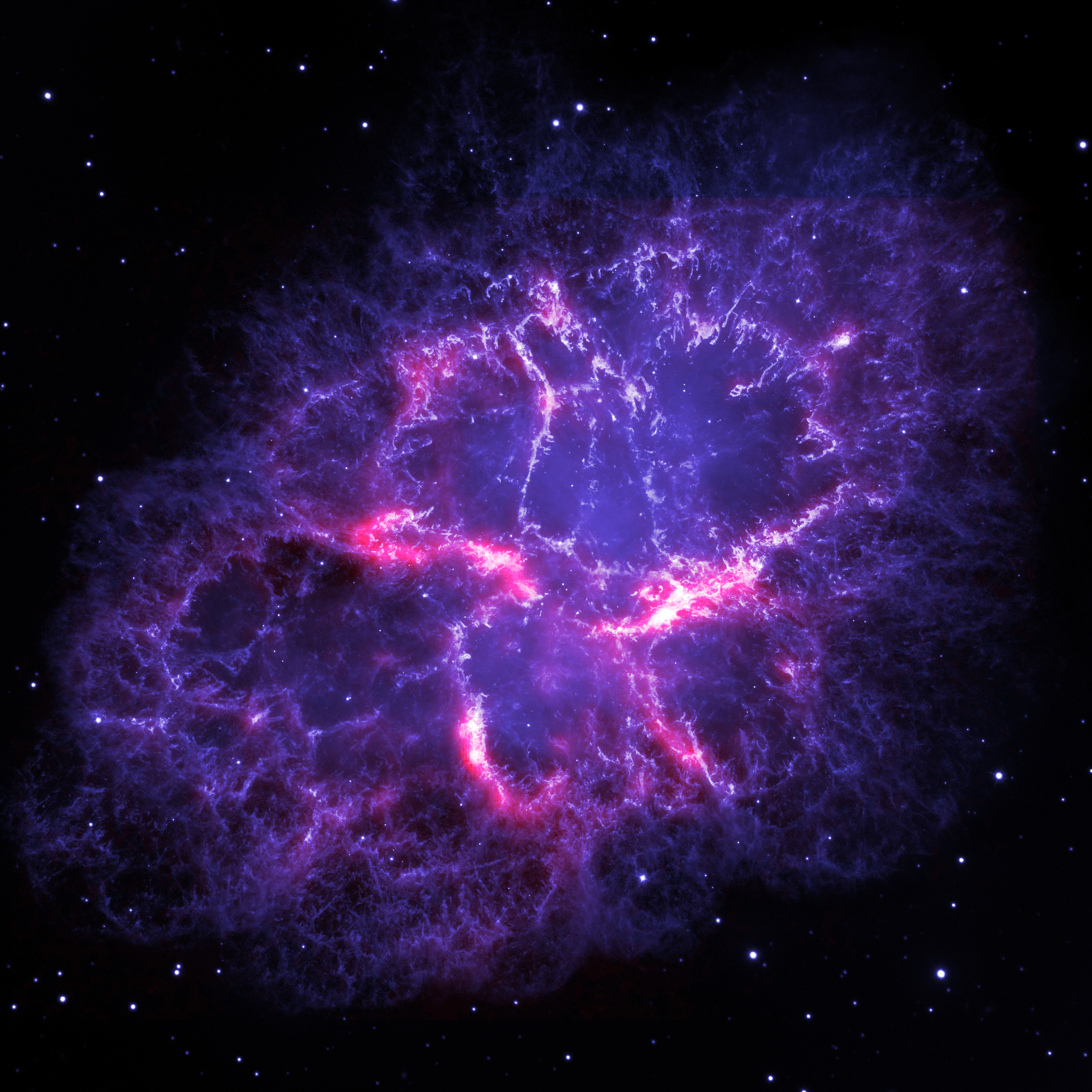
Figure 1: Composite image of the Crab Nebula, obtained by combining a Hubble Space Telescope optical emission line image (blue-white) with a Herschel Space Observatory 70-$\mu$m dust emission image (red), showing the emitting dust to be closely aligned with the optical knots and filaments. The image is 5.65 arcmin on a side; north is up and east is to the left. Credits: Oli Usher (UCL); Herschel Space Observatory, Hubble Space Telescope: ESA, NASA.

The Herschel observations of the Cas A, SN 1987A and Crab supernova remnants that have been summarised above have refocused attention on the potentially significant contribution that core-collapse supernovae can make to interstellar dust budgets. Given the importance of an accurate dust mass estimate for the Crab Nebula, we have constructed a number of gas+dust radiative transfer models for the nebula that use the diffuse radiation field of the pulsar wind nebula (PWN) along with realistic nebular geometries and density distributions. In these models, dust grains with a range of compositions and size distributions are immersed in nebular gas outside the PWN, with the gas either (a) smoothly distributed, or (b) within clumps that mimic the Crab’s highly filamentary structure. We present first our fits to the integrated optical emission line fluxes measured by Smith (2003) for the Crab Nebula, yielding gas-phase elemental abundances and masses in the nebula. We then present the results from our modelling of the infrared spectral energy distribution using several different potential grain species, and compare our derived dust masses with previously published dust mass estimates.

II Input parameters for the gas and dust models

Table 1: Model parameters

	Model i	Model ii	Model iii	Model iv	Model v	Model vi
Density distribution	Smooth	Smooth	Smooth	Clumped	Clumped	Clumped
Total dimensions	4.0$\times$2.9 pc	4.0$\times$2.9 pc	4.0$\times$2.9 pc	4.0$\times$2.9 pc	4.0$\times$2.9 pc	4.0$\times$2.9 pc
Inner axes	1.1$\times$1.1 pc	2.1$\times$1.4 pc	2.3$\times$1.7 pc	3.0$\times$2.0 pc	2.3$\times$1.7 pc	2.3$\times$1.7 pc
H-density	1400 cm-3	775 cm-3	675 cm-3	1700 cm-3	1900 cm-3	1900 cm-3
Radius of each clump				0.037 pc	0.037 pc	0.037 pc
Final gas-phase abundances, by number
Hydrogen	1.00	1.0	1.00	1.00	1.00	1.00
Helium	1.83	1.90	1.90	1.83	1.85	1.85
Carbon	9.7$\times 10^{-3}$	9.3$\times 10^{-3}$	9.3$\times 10^{-3}$	9.7$\times 10^{-3}$	1.02$\times 10^{-2}$	1.02$\times 10^{-2}$
Nitrogen	2.5$\times 10^{-4}$	1.5$\times 10^{-4}$	1.5$\times 10^{-4}$	2.5$\times 10^{-4}$	2.5$\times 10^{-4}$	2.5$\times 10^{-4}$
Oxygen	7.2$\times 10^{-3}$	8.0$\times 10^{-3}$	7.0$\times 10^{-3}$	7.2$\times 10^{-3}$	6.2$\times 10^{-3}$	6.2$\times 10^{-3}$
Neon	2.0$\times 10^{-3}$	4.5$\times 10^{-4}$	4.5$\times 10^{-4}$	2.0$\times 10^{-3}$	4.9$\times 10^{-3}$	4.9$\times 10^{-3}$
Sulphur	4.0$\times 10^{-4}$	5.0$\times 10^{-5}$	5.0$\times 10^{-5}$	4.0$\times 10^{-4}$	4.0$\times 10^{-5}$	4.0$\times 10^{-5}$
Argon	5.0$\times 10^{-5}$	6.0$\times 10^{-6}$	5.0$\times 10^{-5}$	5.0$\times 10^{-5}$	1.0$\times 10^{-5}$	1.0$\times 10^{-5}$

The Crab Nebula is the remnant of a supernova that was recorded in 1054. A distance of 2 kpc is often adopted (Trimble, 1968). It is one of the best-studied objects in the sky, having been observed at all wavelengths from $\gamma$-rays to the radio. It has been suggested to have resulted from a Type IIn-P core-collapse explosion of a progenitor star whose initial mass was $\sim$10 M_⊙ (Smith, 2013). The nebula is rare amongst SNRs in not being collisionally ionized but is instead photoionized by synchrotron radiation from the pulsar wind nebula at the center of the remnant (Hester, 2008).

We have used mocassin (Ercolano et al., 2003, 2005, 2008), a 3D photoionization and dust radiative transfer code which allows for arbitrary gas and dust geometries and density distributions, diffuse radiation fields and multiple point input radiation sources with user-specified spectra, and multiple dust grain species having user-specified grain size distributions. mocassin self-consistently solves the equations of radiative transfer to determine within each cell the degree of ionisation and the gas and dust temperatures, along with the overall line and continuum output spectrum from X-ray to submillimeter (submm) wavelengths of the region being modelled. We used mocassin 2.02.70 to fit the Crab’s observed infrared and submm SED (Temim et al., 2006; Gomez et al., 2012; Planck Collaboration, 2011), along with the integrated optical nebular emission line fluxes measured by Smith (2003).

II.1 The input radiation field and the nebular geometry

The adopted overall geometry for the nebula was an ellipsoid with a major axis diameter of 4.0 pc and a minor axis diameter of 2.9 pc (Hester, 2008). The synchrotron-emitting pulsar wind nebula permeates this volume, which is also partly occupied by the gas corresponding to the observed clumps and filaments.

The pulsar wind nebula’s synchrotron spectrum from 0.36 nm to 1 m that was used for the modelling was a digitized version of the spectrum plotted by Hester (2008). The level of the submillimeter part of the input spectrum needed to be lowered slightly in order to be consistent with recent Planck observations (Planck Collaboration, 2011). The spectrum was scaled to have an integrated luminosity of 1.3$\times 10^{38}$ erg s^-1 (Hester, 2008). The angular extent of the synchrotron emission from the pulsar wind nebula appears to be a function of frequency, with the radio emission extending throughout the 4.0$\times$2.9 pc ellipsoidal nebula (Hester, 2008), while at X-ray wavelengths the PWN has a diameter of $\sim$ 1 pc (Hester et al., 2002).

To investigate the effects of different distributions of gas and dust within the nebula, several shell and PWN geometries were therefore investigated. Table 1 summarises some of the parameters used for the nebular models described below.

1. a smooth shell distribution, with the gas and dust located at a radius of 0.55 pc in a 0.1 pc thick shell (i.e. both inner axes 1.1 pc in length), with the PWN diffuse field radiation field emitting uniformly from within the inner nebular radius of 1.1 pc. This shell geometry was argued for by Čadež et al. (2004) based on their multi-slit spectroscopy and was adopted by Temim & Dwek (2013) for their dust modelling. A shell hydrogen density of 1400 cm^-3 was found to be needed to match the total (dereddened) H$\beta$ flux fom the nebula.

2. a smooth distribution of gas and dust in a shell with inner axis diameters of 2.1$\times$1.4 pc that extends to the outer nebular boundaries, immersed in a diffuse PWN radiation source that also extends to the outer boundaries. This corresponds to the geometry discussed by Davidson & Fesen (1985). A shell hydrogen density of 775 cm^-3 matched the total nebular H$\beta$ flux.

3. a smooth gas and dust distribution in a shell that has inner axes of 2.3$\times$1.7 pc (Lawrence et al., 1995), extending all the way to the outer 4.0$\times$2.9 pc limits of the nebula, as does the PWN diffuse radiation source. A shell hydrogen density of 675 cm^-3 was found to match the total nebular H$\beta$ flux.

4. a clumped shell distribution that has inner axis diameters of 3.0$\times$2.0 pc and extending to the 4.0$\times$2.9 pc outer nebular edges, but in this case with the diffuse radiation source located entirely inside the inner axes of the shell. The degree of clumping is determined by fitting the optical line strengths. A clump filling factor of 0.10 and a clump H-density of 1700 cm^-3 were found to be needed. The clumps are 0.037 pc (3.8 arcsec) in radius. The number of clumps decreases with nebular radius as r^-2. The clumps are modelled using sub-grids, as described by Ercolano et al. (2007b).

5. a clumped shell distribution where the gas and dust clumps start at inner axis diameters of 2.3$\times$1.7 pc (Lawrence et al., 1995), and with an r^-2 distribution of clumps that extends to the 4.0$\times$2.9 pc outer boundaries of the nebula, with a volume filling factor of 0.10. The PWN radiation field is a diffuse source emitting uniformly within a 1.1x1.1 pc diameter sphere at the centre of the nebula. For 0.037-pc radius clumps, a H-density of 1900 cm^-3 within the clumps was found to match the total H$\beta$ flux from the nebula.

6. a clumped shell distribution where the gas and dust clumps start at inner axis diameters of 2.3$\times$1.7 pc (Lawrence et al., 1995), and with an r^-2 distribution of clumps that extends to the 4.0$\times$2.9 pc outer boundaries of the nebula, with a volume filling factor of 0.10. The clumps are immersed in the PWN radiation field emitted from the entire volume of the nebula. For 0.037-pc radius clumps, a H-density of 1900 cm^-3 within the clumps was found to match the total H$\beta$ flux from the nebula.

Our preferred geometries are clumped Models V and VI. A clumped version of smooth Model I could not be constructed: its shell is only 0.1 pc thick and already required a relatively high H-density of 1400 cm^-3 to match the optical line fluxes.

III Modelling the emission line fluxes

As well as aiming to fit the nebular infrared photometric fluxes due to dust emission, we also fitted the emission line fluxes from the ionized gas, principally the optical line fluxes measured for the entire nebula by Smith (2003), which we dereddened using E(B-V) = 0.52 (Miller, 1973) and the Galactic reddening law of Howarth (1983). We assumed an intrinsic Case B H$\alpha$/H$\beta$ flux ratio of 2.85 in order to determine the [N ii] 6584,6548 Å contribution to the dereddened combined H$\alpha$+[N ii] flux, and a Case B H$\gamma$/H$\beta$ flux ratio of 0.47 in order to determine the [O iii] 4363 Å contribution to the dereddened H$\gamma$+[O iii] flux. To diagnose the abundances of carbon and argon, lines of which did not fall within the spectral coverage of Smith (2003), we fitted the [C i] 9824, 9850 Å lines and the [Ar iii] 7136 Å line, using the dereddened line intensities relative to H$\beta$ measured by Rudy et al. (1994) for Knot 6 (FK 6) of Fesen & Kirshner (1982). We note that for FK 10 Rudy et al. (1994) measured [C i] and [Ar iii] intensities relative to H$\beta$ that were 4.0 and 2.2 times higher, respectively, than for FK 6. We used their FK 6 relative line intensities because at shorter wavelengths the FK 6 relative line intensities of Henry et al. (1984) show a better match to those measured for the entire nebula by Smith (2003).

As initial nebular abundances, we used the Crab Nebula ‘Domain 2’ heavy element abundances from Table 2 of MacAlpine & Satterfield (2008). Adopting a distance of 2 kpc, we fitted the dereddened total H$\beta$ flux by varying the value of the density of hydrogen in the smooth shell models, or within the clumps in the clumped shell models. The heavy element abundances were iteratively adjusted in order to match the observed line fluxes, including those sensitive to the nebular temperature. The inferred heavy element abundances, by number, are listed in Table 1. Table 2 presents the dereddened integrated nebular line fluxes, together with the predicted line fluxes from one smooth model (Model III) and from one clumped model (Model VI). The other two smooth models yielded line intensity results that were very similar to those from Model III, while the two other clumped models gave line intensities that were very similar to those listed for Model VI (and Model III). This make it clear that the spectral distribution of the ionizing diffuse radiation field from the PWN is the most important factor in determining the emitted nebular spectrum.

Table 2: Dereddened and modelled absolute H$\beta$ fluxes, plus dereddened and modelled line strengths relative to H$\beta$.

Species	Wavelength	Dereddened	Modelled Flux	Dered/Model	Modelled Flux	Dered/Model
	[Å]	Flux1	Smooth iii		Clumped vi
H$\beta$	4861	7.85$\times 10^{-11}$	6.32 $\times 10^{-11}$	1.24	7.24 $\times 10^{-11}$	1.08
[O ii]	3726+3729	18.11	20.1	0.90	18.86	1.07
[Ne iii]	3869	4.65	3.79	1.23	3.99	1.17
[S ii]	4069+4076	0.37	0.32	1.16	0.36	1.03
[O iii]	4363	0.57	0.54	1.06	0.47	1.20
He i	4471	0.37	0.43	0.86	0.37	1.01
He ii	4686	0.78	0.79	0.98	0.79	0.99
H$\beta$	4861	1.00	1.00	1.00	1.00	1.00
[O iii]	5007	11.92	9.57	1.24	9.9	1.19
[N i]	5198+5200	0.13	0.14	0.93	0.15	0.87
[N ii]	5755	0.093	0.086	1.08	0.076	1.22
[O i]+[S iii]	6300,6363+6312	1.23	1.63	0.75	1.21	1.02
H$\alpha$	6563	2.85	2.92	0.98	2.95	0.97
[N ii]	6548+6584	6.87	6.38	1.08	5.70	1.06
[S ii]	6717+6731	4.31	3.98	0.90	4.08	0.94
[Ar iii]	7136	0.34	0.33	1.04	0.41	0.84
[C i]	9824+9850	0.36	0.66	0.55	0.28	1.29

• ¹ Integrated line fluxes for entire nebula are from Smith (2003), dereddened using E(B-V) = 0.52; except for [C i] 9824+9850 and [Ar iii] 7136 relative fluxes, which are from Rudy et al. (1994). First row fluxes are in ergs cm^-2 s^-1; the fluxes in the remaining rows are relative to H$\beta$=1.00.

Table 3: Gas phase elemental masses in the Crab Nebula

?	Model i	Model ii	Model iii	Model iv	Model v	Model vi
	Mass (M⊙)	Mass (M⊙)	Mass (M⊙)	Mass (M⊙)	Mass (M⊙)	Mass (M⊙)
Hydrogen	1.8	5.53	4.47	0.8	0.81	0.81
Helium	13.2	42	33.97	5.86	5.99	5.99
Carbon	0.21	0.62	0.49	9.3$\times 10^{-2}$	9.91$\times 10^{-2}$	9.91$\times 10^{-2}$
Nitrogen	6.3$\times 10^{-3}$	1.2$\times 10^{-2}$	9.39$\times 10^{-3}$	2.8$\times 10^{-3}$	2.84$\times 10^{-3}$	2.84$\times 10^{-3}$
Oxygen	0.2	0.71	0.5	9.2$\times 10^{-2}$	7.94$\times 10^{-2}$	7.94$\times 10^{-2}$
Neon	0.05	5.0$\times 10^{-2}$	0.04	3.2$\times 10^{-2}$	7.8$\times 10^{-2}$	7.8$\times 10^{-2}$
Sulphur	0.02	8.8$\times 10^{-3}$	7.15$\times 10^{-3}$	1.02$\times 10^{-2}$	1.04$\times 10^{-3}$	1.04$\times 10^{-3}$
Argon	3.1$\times 10^{-3}$	1.2-3	6.48$\times 10^{-3}$	1.4$\times 10^{-3}$	2.9$\times 10^{-3}$	2.9$\times 10^{-3}$
Total	15.5	48.9	40.1	6.89	7.02	7.02

Table 4: Gas-phase elemental ion fractions for the best-fit clumpy model vi

	Neutral	$1^{+}$	2+	3+	4+	5+
Hydrogen	0.130	0.870
Helium	0.332	0.630	3.77$\times 10^{-2}$
Carbon	1.01$\times 10^{-2}$	0.730	0.248	2.08$\times 10^{-2}$	2.01$\times 10^{-6}$	1.04$\times 10^{-10}$
Nitrogen	1.04$\times 10^{-2}$	0.708	0.237	5.39$\times 10^{-3}$	1.17$\times 10^{-6}$	2.34$\times 10^{-9}$
Oxygen	0.144	0.721	0.107	2.75$\times 10^{-3}$	1.05$\times 10^{-6}$	7.37$\times 10^{-8}$
Neon	0.114	0.772	0.113	3.72$\times 10^{-4}$	4.10$\times 10^{-6}$	9.93$\times 10^{-9}$
Sulphur	0.198	0.440	0.299	7.05$\times 10^{-3}$	3.34$\times 10^{-5}$	5.66$\times 10^{-8}$
Argon	2.31$\times 10^{-5}$	0.116	0.702	0.178	2.31$\times 10^{-3}$	4.25$\times 10^{-5}$

III.1 Results from the nebular gas-phase modelling

From Table 3, the total nebular gas mass required to match the observed line fluxes ranges from 15.5 M$\odot$ to 49 M$\odot$ for the three smoothly distributed models, whereas for the clumped models the total gas mass is only 6.9 M$\odot$ to 7.0 M$\odot$. The clumped model gas masses are consistent with the 8-10 M$\odot$ mass estimated for the Crab Nebula’s progenitor star (Smith 2013 and references therein), whereas the smooth models are clearly ruled out. Optical emission line images of the Crab Nebula (e.g. Figure 1) also clearly rule out a smooth distribution for the emitting gas.

Table 4 presents the global elemental ion fractions obtained from our clumped Model VI for the Crab Nebula (the ion fraction patterns are very similar for its smooth model equivalent, Model III). Most elements are found to have a neutral faction of about 10%, with the exception of helium, whose neutral fraction is significantly higher, at 33%. A consequence of the high helium neutral fraction in the Crab is that standard abundance analyses based on recombination lines of H⁺, He⁺ and He²⁺ will underestimate the true He/H ratios. We find a helium mass fraction of 85% (Table 3), in agreement with the 89% derived by MacAlpine & Satterfield (2008) from their photoionization modelling of spectra from many locations within the nebula. They also found that the majority of their locations (their ‘Domain 2’) had C/O ratios greater than unity, both by number and by mass. Our clumped Models V and VI for the entire nebula are consistent with those results, yielding a C/O ratio of 1.65 by number. The mass ratio of C/(H+He) is enhanced by a factor 6.2 in the Crab Nebula relative to the solar abundances of Asplund et al. (2009), while the O/(H+He) mass ratio is enhanced by only a factor of 2.3. The corresponding mass ratios of neon, sulphur and argon for the Crab are enhanced by factors of 3.8, 4.9 and 3.1 relative to solar, while nitrogen is depleted by a factor of 1.7.

C/O mass ratios exceeding unity are not currently predicted by any supernova nucleosynthesis models, for any mass of progenitor star. For the CCSN yields tabulated by Woosley & Weaver (1995), the ejecta C/O mass ratio did increase with decreasing progenitor mass but for the lowest mass cases that they treated (11-12 M_⊙) the predicted C/O mass ratio was 0.39, for the case of initial solar metallicity, and the predicted carbon yield was only 0.053 M_⊙, i.e. lower than the Crab Nebula’s gas-phase carbon mass alone of 0.099 M_⊙. In addition, their 11 M_⊙ model predicted an ejecta He/H mass ratio of 0.67, versus the very much larger He/H mass ratio of 7.3 found here for the Crab Nebula. For the lowest progenitor mass model (13 M_⊙) of Thielemann et al. (1996), an even lower ejecta carbon mass and C/O mass ratio was predicted than for the Woosley & Weaver (1995) model of the same mass. The 13 M_⊙ model of Nomoto et al. (2006) predicted a He/H mass ratio of 0.7 and a C/O mass ratio of 0.5, also too low compared to Crab Nebula ratios. The trend for predicted carbon yields to increase with decreasing progenitor mass suggests that it would be useful to calculate yields for CCSN progenitor masses down to 8 M_⊙. However, we conclude that since no existing CCSN yield predictions match the case of the Crab Nebula, they therefore do not provide useful constraints on the total masses of heavy elements that could be in the gas phase or tied up within dust grains in the Crab Nebula.

From an empirical analysis, Fesen et al. (1997) estimated a total gas mass of 4.6$\pm$1.8 M_⊙ for the Crab Nebula, of which 1.5 M_⊙ was estimated to be in neutral filaments. From our clumped photoionization model we find a total gas mass 7.0 M_⊙, of which 2.1 M_⊙ is neutral (Tables 3 and 4). Fesen et al. (1997) used an observed total H$\beta$ flux of 1.78$\pm 0.20\times 10^{-11}$ ergs cm^-2 s^-1, from MacAlpine & Uomoto (1991), versus the value of 1.38$\pm 0.07\times 10^{-11}$ ergs cm^-2 s^-1 from Smith (2003) used here. Kirshner (1974) measured a total H$\beta$ flux of 1.30$\pm 0.40\times 10^{-11}$ ergs cm^-2 s^-1, while Davidson (1987) estimated 1.16$\pm 0.12\times 10^{-11}$ ergs cm^-2 s^-1. We adopt a factor of 1.15 uncertainty in the total H$\beta$ flux, which corresponds to a factor of 1.15^1/2 = 1.07 uncertainty in the total nebular gas mass of 7.0$\pm 0.5$ M_⊙.

The photoionization models described above included the dust grain components that are described in the next Section. However, running the models without dust made an insignificant difference to the emission line fits, i.e. dust does not compete significantly for the photons that determine the global gas-phase ionization balance and line emission from the nebula. By contrast, for a model run without gas, the dust emission was a factor of 1.17 lower than for the gas+dust model, indicating that absorption of nebular gaseous emission lines makes a significant contribution to the dust luminosity.

III.1.1 Argon and ArH⁺

Barlow et al. (2013) discovered the noble gas molecular ion ³⁶ArH⁺ in the Crab Nebula, via the detection of its J=1-0 and 2-1 rotational emission lines in Herschel-SPIRE FTS spectra. We therefore included argon in our photoionization modelling of the nebula. As noted above, for Knot FK 6, typical of the nebula as a whole, argon’s mass fraction was found to be enhanced by a factor of three relative to solar. However, [Ar iii] relative line intensities at Knot FK 10, where ArH⁺ emission is strongest, are a factor of two higher than at FK 6, suggesting a larger enhancement of the argon abundance there. Following the detection of ArH⁺ emission in the Crab Nebula, Schilke et al. (2014) were able to use a previously unidentified interstellar absorption feature, now identified as due to ground-state absorption by the J=1-0 rotational line of ArH⁺, to diagnose the physical conditions in the absorbing interstellar clouds. They concluded that the formation reaction H₂ + Ar⁺ $\rightarrow$ H + ArH⁺ must take place in regions where hydrogen is overwhelmingly in the form of neutral atoms. This is relevant to the Crab Nebula, since photoionization models predict the existence of significant zones of atomic hydrogen (see Table 4 and Richardson et al. (2013)). Richardson et al. concluded from their models that the Crab Nebula knots from which H₂ line emission had been detected were almost entirely atomic. The likelihood that ArH⁺ also forms and emits in these regions should be investigated with further modelling.

IV Modelling the dust component

Our smooth and clumped radiative transfer models treat both gas and dust and, as described below, have been run with a wide range of dust grain parameters in order to find optimum fits to the observed infared spectral energy distribution of the Crab Nebula in order to diagnose the mass of dust present.

From an analysis of Spitzer spectra, Temim et al. (2012) found the majority of the warmer dust in the Crab nebula to be located in the clumpy filamentary structures. This conclusion was supported by synchrotron-subtracted Spitzer and Herschel images presented by Gomez et al. (2012), which showed both the warm and cool dust to be concentrated in the nebular filaments. Figure 1 shows the far-infrared dust emission from the Crab Nebula to be closely aligned with the knots and filaments that dominate optical emission line images of the nebula. Given this evidence and the fact that smooth models require an implausibly large nebular gas mass, we will concentrate below on the results from our clumped gas+dust models.

IV.1 The grain species and their optical constants

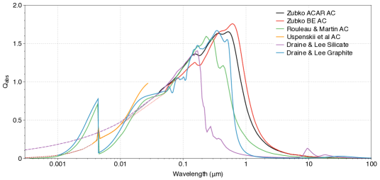
Figure 2: Q${}_{\text{abs}}$($\lambda$) versus wavelength for carbon grains (apart from the Draine & Lee silicate) of radius 0.1 $\mu$m, with optical constants taken from the labelled sources discussed in Section 4.1. Dashed or dotted portions use extrapolated or interpolated optical constants (see text).

As discussed in Section 3.1, the Crab Nebula is carbon-rich, with C/O$>$1 by number (Table 2), though with a few oxygen-rich zones (MacAlpine & Satterfield, 2008). Since its Spitzer IRS spectra show no features at 10 or 20 $\mu$m attributable to silicate Si-O stretching or bending modes (Temim et al., 2006, 2012), we have focused largely on amorphous carbon as the dominant grain species. However, we did construct some models that included silicates, using the silicate optical constants of Draine & Lee (1984), from whom we also adopted the optical constants for our graphite grain models.

For their amorphous carbon models, Temim & Dwek (2013) used optical constants from Rouleau & Martin (1991) (their ‘AC1’) and from Zubko et al. (1996) (‘BE’). For comparison purposes we also ran models using the Rouleau & Martin (1991) AC1 amorphous carbon constants, based largely on optical constants measured by Bussoletti et al. (1987), as well as models with the Zubko et al. (1996) BE amorphous carbon optical constants. The latter were based on data measured by Colangeli et al. (1995) for carbon particles produced from burning benzene samples. We additionally ran models using the Zubko et al. (1996) ‘ACAR’ optical constants, based also on measurements by Colangeli et al. (1995), this time for particles produced via an electrical discharge through carbon electrodes in argon gas.

The ACAR and BE amorphous carbon optical constants of Zubko et al. (1996) have no data points for wavelengths shorter than 40 nm and 54 nm, respectively. Since a significant fraction of the Crab PWN luminosity is emitted shortwards of these wavelengths, we extended the BE and the ACAR optical constants down to shorter wavelengths using the 2.8 nm to 30 nm amorphous carbon optical constant measurements of Uspenskii et al. (2006), which are presented in the Appendix. Also listed there are n and k optical constants suitable for Zubko et al. (1996) BE and ACAR grains over the 0.35-54 nm wavelength range, obtained as described in the Appendix. Figure 2 shows a comparison from 0.35 nm to 1000 $\mu$m between the absorption efficiencies of 0.1-$\mu$m radius amorphous carbon grains for the supplemented Zubko et al. (1996) BE and ACAR optical constants, as well as for the optical constants of Rouleau & Martin (1991). As the latter do not have any data points longwards of 300 $\mu$m, we extrapolated them to 1000 $\mu$m by fitting power laws to their n and k data points from 10-300 $\mu$m, since they change smoothly over this range.

Inspection of the absorption efficiencies plotted in Figure 2 shows significant differences between the supplemented Zubko et al. (1996) BE and ACAR efficiencies and those of Rouleau & Martin (1991), especially at wavelengths below 20 nm and longwards of 310 nm. For wavelengths below 100 nm we prefer the supplemented BE and ACAR data, since we extended these below 30 nm by using experimental optical constants for amorphous carbon measured by Uspenskii et al. (2006). In particular, the Uspenskii et al. (2006) data show a much smaller discontinuity at the carbon atom K-edge at 282 eV (4.4 nm) than the data of Rouleau & Martin (1991). Since K-shell edges correspond to the ejection by photons of inner shell electrons from atoms, the vast majority of the photon energy does not go into grain heating but in to raising the K-shell electron out of its potential well. Therefore for grain heating calculations, the inclusion of K-shell absorption peaks will significantly overestimate the amount of grain heating that results.

For wavelengths longwards of 310 nm, the ‘AC1’ amorphous carbon optical constants presented by Rouleau & Martin (1991) made use of laboratory measurements of extinction efficiencies published by Bussoletti et al. (1987). The latter group subsequently obtained new laboratory measurements of mass extinction coefficients for different types of amorphous carbon particles (Colangeli et al., 1995). They noted that their new data agreed with the measurements of Koike et al. (1980) for similar particles but not with their own (Bussoletti et al., 1987) earlier measurements. The newer data of (Colangeli et al., 1995) were used to produce the amorphous carbon optical constants presented by Zubko et al. (1996), and overall we consider these, and their extensions here to shorter wavelengths, to provide the most reliable data available for amorphous carbon.

For our modelling we adopted a mass density of 1.85 g cm^-3 for amorphous carbon, 2.2 g cm^-3 for graphite, and 3.3 g cm^-3 for silicate.

IV.2 Fitting the observed infrared and submillimeter photometric continuum fluxes

Table 5: Continuum IR Fluxes from the Crab Nebula

Wavelength	Total Flux1	Uncertainty	Dust Flux	Instrument2
($\mu$m)	(Jy)	(Jy)	(Jy)
3.6	12.6	0.22		Spitzer
4.5	14.4	0.26		Spitzer
5.8	16.8	0.10		Spitzer
8.0	18.3	0.13		Spitzer
24	46.4	8.0	17.2	Spitzer
70	202.4	20	156.8	Herschel
100	196.5	20	143.6	Herschel
160	141.8	15	77.5	Herschel
250	103.4	7.2	25.9	Herschel
350	102.4	7.2	13.2	Herschel
350	99.3	2.1	10.1	Planck
500	129.0	9.0		Herschel
550	117.7	2.1		Planck
850	128.6	3.1		Planck
1382	147.2	3.1		Planck

• ¹ The 24-, 70- and 100-$\mu$m fluxes have been corrected for line emission following Table 2 of Gomez et al. (2012).

• ² Spitzer data: Temim et al. (2006); Herschel data: Gomez et al. (2012); Planck data: Planck Collaboration (2011).

The model dust SEDs were fitted to the observed infrared and submm photometric fluxes, using observations made by Spitzer (Temim et al., 2006), Herschel (Gomez et al., 2012) and Planck (Planck Collaboration, 2011), along with the mean synchrotron-subtracted Spitzer-IRS continuum spectrum of Temim & Dwek (2013), to better constrain the warm dust emission. The 24-, 70- and 100-$\mu$m points have been corrected for line emission, using the line contribution factors listed in Table 2 of Gomez et al. (2012). The dust+synchrotron continuum fluxes are listed in Table 5, along with 24-350-$\mu$m dust continuum fluxes obtained by subtracting the synchrotron fluxes listed in Table 4 of Gomez et al. (2012). For a distance of 2 kpc, the total luminosity emitted by dust at infrared wavelengths is 1190 L_⊙, corresponding to the absorption and reradiation of 28% of the luminosity of the pulsar wind nebula emitted between 0.1 nm and 1.0 $\mu$m.

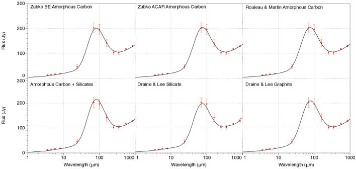
Figure 3: The best fit overall SEDs for clumped model vi. The SEDs corresponds to the parameters in Table 7, for the different grain types described in Section 4.1. The observational data points are described in Section 4.2.

Fitting the models to the observations was done by assuming that the uncertainties associated with each of the observed fluxes were Gaussian, sampling randomly within the allowed observational uncertainty range to generate 1000 separate versions of the SED. These were compared to the model SEDs and the set of model parameters generating the lowest mean $\chi^{2}$ value was taken to be the most likely. The best fit models to the Crab Nebula’s infrared SED are shown in Figure 3 for a number of different grain types, while the dust parameters used to obtain these fits are listed in Tables 6 and 7. The uncertainties listed for the derived dust masses are based on the combination in quadrature of the uncertainties in the dust continuum fluxes between 70 and 160-$\mu$m and the uncertainties in fitting the SED for each grain/nebular model.

When models were initially run with a standard MRN grain size distribution (Mathis, Rumpl, & Nordsieck, 1977), i.e. $n(a)\propto a^{-\alpha}$ with $\alpha$ = 3.5, a_min = 0.005 $\mu$m and a_max = 0.25 $\mu$m, the dust energy distribution was found to peak at too short a wavelength. To better fit the observed peak, which is at about 70 $\mu$m, the maximum grain radius had to be increased to provide larger, cooler, grains, and the power-law slope $\alpha$ had to be decreased, increasing the relative number of larger grains. Since colder dust emits less efficiently at a given wavelength than warmer dust, the dust mass required to fit the observed fluxes also had to increase. For a number of different grain types, $\alpha$ = 2.7-3.0 was found to provide the best fit to the observed SED (see Tables 6 and 7). For values of $\alpha<$ 4, the largest grains dominate the total dust mass. There is a degeneracy between the maximum grain size and the slope of the power law, $\alpha$, however better fits to both the mid and far infrared components of the SED were achieved with a lower a_max and $\alpha$. The value of a_max was varied between 0.1 and 2 $\mu$m, a_min was varied between 0.0005 and 0.1 $\mu$m and $\alpha$ was varied between 2.4 and 4.

IV.3 The Mass of Dust

Table 6: Dust masses for the best fit gas+dust smooth models for the Crab Nebula

Model i Čadež et al. (2004) shell: 0.1 pc thick at 0.55 pc radius with central heating source
Optical Constants	amin	amax	$\alpha$	Mdust	$\chi^{2}$
Zubko et al. ACAR	0.005${{}^{+0.005}_{-0.001}}$ $\mu$m	0.7 $\pm$ 0.01 $\mu$m	2.7 $\pm$ 0.1	0.21 $\pm$ 0.02 M⊙	5.54
Zubko et al. BE	0.005${{}^{+0.005}_{-0.001}}$ $\mu$m	0.5  $\pm$ 0.01 $\mu$m	2.7 $\pm$ 0.1	0.18 $\pm$ 0.01 M⊙	3.39
Rouleau & Martin AC1	0.01 $\pm$ 0.01  $\mu$m	0.8 $\pm$ 0.01 $\mu$m	2.9 $\pm$ 0.1	0.10 $\pm$ 0.01 M⊙	5.21
Mixed Chemistry	0.01 $\mu$m	1.0 $\mu$m	3.0 $\pm$ 0.1	0.25 $\pm$ 0.02 M⊙	5.23
				0.05 $\pm$ 0.01 M⊙ Zubko BE
				0.14 $\pm$ 0.01 M⊙ DL silicates
Draine & Lee Silicate	0.01 $\pm$ 0.01 $\mu$m	0.9 $\pm$ 0.01 $\mu$m	3.5 $\pm$ 0.1	0.33 $\pm$ 0.04 M⊙	6.11
Draine & Lee Graphite	0.001 $\pm$ 0.001 $\mu$m	0.25 $\pm$ 0.01 $\mu$m	2.8 $\pm$ 0.1	0.11 $\pm$ 0.01 M⊙	4.57
Model ii - Davidson & Fesen (1985): shell: 2.1x1.4pc to 4.0x2.9 pc
Optical Constants	amin	amax	$\alpha$	Mdust	Reduced $\chi^{2}$
Zubko et al. ACAR	0.01 $\pm$ 0.01 $\mu$m	1.0 $\pm$ 0.01 $\mu$m	2.9 $\pm$ 0.1	0.18 $\pm$ 0.03 M⊙	9.9
Zubko et al BE	0.01 $\pm$ 0.01 $\mu$m	0.5 $\pm$ 0.01 $\mu$m	2.9 $\pm$ 0.1	0.14 $\pm$ 0.02 M⊙	9.7
Rouleau & Martin AC1	0.01 $\pm$ 0.01 $\mu$m	1.0 $\pm$ 0.01 $\mu$m	3.0 $\pm$ 0.1	0.08 $\pm$ 0.01 M⊙	12.1
Mixed Chemistry	0.01 $\pm$ 0.01 $\mu$m	0.8 $\pm$ 0.01 $\mu$m	3.0 $\pm$ 0.1	0.29 $\pm$ 0.02 M⊙	6.31
				0.10 $\pm$ 0.01 M⊙ Zubko BE
				0.19 $\pm$ 0.01 M⊙ DL silicates
Draine & Lee Silicate	0.01 $\pm$ 0.01 $\mu$m	1.0 $\pm$ 0.01 $\mu$m	3.5 $\pm$ 0.1	0.48 $\pm$ 0.1M⊙	11.3
Draine & Lee Graphite	0.001 $\pm$ 0.001 $\mu$m	0.25 $\pm$ 0.01 $\mu$m	3.0 $\pm$ 0.1	0.09 $\pm$ 0.01 M⊙	11.0
Model iii - Lawrence et al. (1995) shell: 2.3x1.7 pc to 4.0x2.9 pc
Optical Constants	amin	amax	$\alpha$	Mdust	Reduced $\chi^{2}$
Zubko et al. ACAR	0.01 $\pm$ 0.01 $\mu$m	0.7 $\pm$ 0.01 $\mu$m	2.9 $\pm$ 0.1	0.14 $\pm$ 0.04 M⊙	5.22
Zubko et al. BE	0.005 $\pm$ 0.005 $\mu$m	0.5 $\pm$ 0.01 $\mu$m	2.8 $\pm$ 0.1	0.11 $\pm$ 0.02 M⊙	5.97
Rouleau & Martin AC1	0.01 $\pm$ 0.01 $\mu$m	0.7 $\pm$ 0.01 $\mu$m	3.0 $\pm$ 0.1	0.06 $\pm$ 0.01 M⊙	4.89
Mixed Chemistry	0.01 $\mu$m	0.8 $\mu$m	3.0 $\pm$ 0.1	0.21 $\pm$ 0.02 M⊙	6.92
				0.07 $\pm$ 0.01 M⊙ Zubko BE
				0.14 $\pm$ 0.01 M⊙ DL silicates
Draine & Lee Silicate	0.001 $\pm$ 0.001 $\mu$m	0.9 $\pm$ 0.01 $\mu$m	3.5 $\pm$ 0.1	0.37 $\pm$ 0.06 M⊙	5.14
Draine & Lee Graphite	0.001 $\pm$ 0.001 $\mu$m	0.25 $\pm$ 0.01 $\mu$m	2.9 $\pm$ 0.1	0.07 $\pm$ 0.01 M⊙	6.66

Table 7: Dust masses for the best fit gas+dust clumped models for the Crab Nebula

Model iv - Clumps beyond the ionising radiation: 3.0$\times$2.0 pc to 4.0$\times$2.9 pc
Optical Constants	amin	amax	$\alpha$	Mdust	$\chi^{2}$
Zubko AC	0.07 $\pm$ 0.01 $\mu$m	1.0 $\pm$ 0.01 $\mu$m	2.9 $\pm$ 0.1	0.40 $\pm$ 0.08 M⊙	5.39
Zubko BE	0.07 $\pm$ 0.01 $\mu$m	0.2 $\pm$ 0.01 $\mu$m	2.9 $\pm$ 0.1	0.30 $\pm$ 0.06 M⊙	5.52
Rouleau & Martin AC	0.07 $\pm$ 0.01 $\mu$m	1.0 $\pm$ 0.01 $\mu$m	3.0 $\pm$ 0.10	0.24 M⊙	4.35
Mixed Chemistry	0.07 $\pm$ 0.01 $\mu$m	1.0 $\pm$ 0.01 $\mu$m	3.0 $\pm$ 0.1	0.78 M⊙	6.61
				0.18 $\pm$ 0.03 M⊙ Zubko BE
				0.60 $\pm$ 0.03 M⊙ DL silicates
Draine & Lee Silicate	0.07 $\pm$0.01 $\mu$m	1.0 $\pm$0.01 $\mu$m	3.5 $\pm$ 0.1	1.5 M⊙	4.38
Draine & Lee Graphite	0.001 $\pm$0.01 $\mu$m	0.25 $\pm$0.01 $\mu$m	3.0 $\pm$ 0.1	0.40 M⊙	3.22
v Clumped Lawrence et al. (1995) shell: 2.3x1.7 pc to 4.0x2.9 pc - 1.1x1.1 source
Optical Constants	amin	amax	$\alpha$	Mdust	$\chi^{2}$
Zubko et al. ACAR	0.005${{}^{+0.005}_{-0.001}}$$\mu$m	0.7 $\pm$ 0.01  $\mu$m	2.7 $\pm$ 0.1	0.27 $\pm$ 0.04 M⊙	6.08
Zubko et al. BE	0.005${{}^{+0.005}_{-0.001}}$ $\mu$m	0.5 $\pm$ 0.01 $\mu$m	2.7 $\pm$ 0.1	0.20 $\pm$ 0.03 M⊙	5.99
Rouleau & Martin AC1	0.01 $\pm$ 0.01 $\mu$m	0.8 $\pm$ 0.01 $\mu$m	2.9 $\pm$ 0.1	0.17 $\pm$ 0.03 M⊙	4.98
Mixed Chemistry	0.01 $\pm$ 0.01  $\mu$m	1.0 $\pm$ 0.01 $\mu$m	3.0 $\pm$ 0.1	0.58 $\pm$ 0.05 M⊙	5.76
				0.13 $\pm$ 0.02 M⊙ Zubko BE
				0.47 $\pm$ 0.03 M⊙ DL silicates
Draine & Lee Silicate	0.01 $\pm$ 0.005 $\mu$m	0.9 $\pm$ 0.01 $\mu$m	3.5 $\pm$ 0.1	1.10 $\pm$ 0.19 M⊙	5.44
Draine & Lee Graphite	0.001 $\pm$ 0.001 $\mu$m	0.25 $\pm$ 0.01 $\mu$m	2.8 $\pm$ 0.1	0.2-$\pm$ 0.03 M⊙	6.03
Model vi Clumped Lawrence et al. (1995) shell: 2.3x1.7 pc to 4.0x2.9 pc - full nebula source
Optical Constants	amin	amax	$\alpha$	Mdust	$\chi^{2}$
Zubko et al. ACAR	0.005${{}^{+0.005}_{-0.001}}$ $\mu$m	0.7 $\pm$ 0.01 $\mu$m	2.7 $\pm$ 0.1	0.25 $\pm$ 0.04 M⊙	5.72
Zubko et al. BE	0.005${{}^{+0.005}_{-0.001}}$ $\mu$m	0.5 $\pm$ 0.01 $\mu$m	2.7 $\pm$ 0.1	0.18 $\pm$ 0.03 M⊙	4.87
Rouleau & Martin AC1	0.01 $\pm$ 0.01 $\mu$m	0.8 $\pm$ 0.01 $\mu$m	2.9 $\pm$ 0.1	0.15 $\pm$ 0.03 M⊙	4.38
Mixed Chemistry	0.01 $\pm$ 0.01 $\mu$m	1.0 $\pm$ 0.01 $\mu$m	3.0 $\pm$ 0.1	0.50 $\pm$ 0.05 M⊙	6.62
				0.11 $\pm$ 0.02 M⊙ Zubko BE
				0.39 $\pm$ 0.03 M⊙ DL silicates
Draine & Lee Silicate	0.01 $\pm$ 0.01  $\mu$m	0.9 $\pm$ 0.01 $\mu$m	3.5 $\pm$ 0.1	0.98 $\pm$ 0.19 M⊙	5.12
Draine & Lee Graphite	0.001 $\pm$ 0.001  $\mu$m	0.25 $\pm$ 0.01 $\mu$m	2.8 $\pm$ 0.1	0.17 $\pm$ 0.03 M⊙	6.42

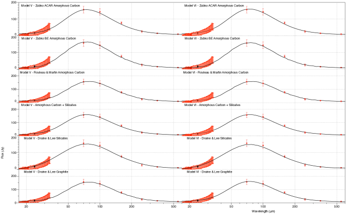
Figure 4: The best fit synchrotron subtracted clumped models v (left column) and vi (right column) dust fluxes. The dust SEDs corresponding to the parameters in Table 7, for the different grain types described in Section 4.1. The observational data points are described in Section 4.2 plotted with the photometric points and Spitzer-IRS spectrum.

The flux from optically thin dust emission is linearly proportional to the total number of dust grains, irrespective of whether they are in clumps. The reason that our clumped models have larger dust masses than our smooth models (a factor of $\sim$ 1.7 larger in the case of amorphous carbon models III vs. VI with Zubko ACAR and BE grain constants) is that the short wavelength radiation that heats the grains is attenuated by the gas and dust within the clumps, leading to cooler grains in the clump interiors than would otherwise be the case. Since cooler grains emit less efficiently, a larger mass of grains needs to be accommodated when matching a given far-infrared flux.

Recombination and forbidden line emissivities are proportional to gas density squared, enabling the higher gas density clumped model to fit the observed line fluxes with a plausible nebular gas mass while ruling out smoothly distributed models because they require an implausible 16-49 M_⊙ of gas in the Crab, versus 7 M_⊙ of gas for the best-fit clumped models (Table 3). We therefore consider that only the clumped models in Table 7 are realistic. In addition, since the Crab Nebula has carbon-rich gas-phase abundances (C/O $>$ 1; Table 1), the models with carbon grains are preferred over those with silicates.

Models V and VI have the same distribution of dust and gas, but have different heating sources, with model V having a centrally located source 1.1$\times$1.1 pc in diameter whilst model VI has the clumps embedded in a source that extends out to 4.0$\times$2.9 pc. The extra heating caused by the clumps being embedded in the radiation source rather than outside it means that Model VI requires less dust to fit the observed SED than Model V. The spectral shape and luminosity of the radiation field have a far greater effect on the mass of dust derived for the Crab Nebula than any of the geometrical and density effects investigated.

Focusing on the carbon grain models, since the Rouleau & Martin (1991) amorphous carbon and Draine & Lee (1984) graphite optical constants both include inappropriate K-shell absorption peaks (Figure 2) that in fact do not contribute significantly to grain heating (see the discussion in Section 4.1), the Zubko et al. (1996) BE and ACAR amorphous carbon models are our preferred grain species, in clumped Models V or VI. These models yield a total dust mass in the Crab Nebula of 0.18 - 0.27 M_⊙ (Table 7).

Since MacAlpine & Satterfield (2008) found a few O-rich regions in the predominantly C-rich Crab Nebula, a further possibility is our ‘Mixed Model’, with 0.11 M_⊙ of Zubko et al. (1996) BE amorphous carbon and 0.39 M_⊙ of Draine & Lee (1984) silicates for Model VI’s geometry, or 0.13 M_⊙ and 0.47 M_⊙, respectively, for Model V’s geometry. In order to compare with our Draine & Lee (1984) silicate models, we also ran models with silicate optical constants from Laor & Draine (1993). The resulting silicate dust mass fits were 6% higher than those found with the silicate optical constants of Draine & Lee (1984).

Allowing for the 0.099 M_⊙ of gas-phase carbon in the nebula for clumped Models V or VI (Table 3), the minimum total mass of carbon in the Crab Nebula is 0.28 M_⊙. As discussed in Section 3.1, we do not consider that the low carbon yields predicted by the 11-13-M_⊙ core-collapse SN models of Woosley & Weaver (1995), Thielemann et al. (1996) and Nomoto et al. (2006) provide a useful constraint on the mass of carbon that can be in dust, since their predicted C/O and He/H mass ratios are much smaller than those found in the Crab Nebula.

For clumped Model V with Zubko et al. (1996) BE amorphous carbon grains (Table 7), the gas and dust masses in each clump were respectively 6.08$\times 10^{-3}$ M_⊙ and 1.68$\times 10^{-4}$ M_⊙, for a gas to dust mass ratio of 36, and the V-band dust optical depth from the edge to the centre of each clump was $\tau_{V}$ = 1.12. Following the detection by Woltjer & Veron-Cetty (1987) of absorption attributable to dust at the position of a bright [O iii] filament in the Crab Nebula, Fesen & Blair (1990) measured angular diameters ranging from 0.9 to 4.8 arcsec for 24 ‘dark spots’ in the Crab Nebula. For comparison, the 0.037-pc radius clumps adopted for our clumped models would have an angular radius of 3.8 arcsec at a distance of 2 kpc.

IV.3.1 Comparison with previous dust mass estimates

Since cool dust emits less efficiently than warm dust, larger dust masses are needed to fit far-infrared fluxes than are required to fit similar fluxes at shorter infrared wavelengths. So observations extending out to far-infrared and submillimeter wavelengths are often necessary in order to fully characterize nebular dust masses. In our comparisons below, we will focus on dust mass estimates made assuming carbon grains.

Prior to the launch of Herschel, the longest infrared wavelengths that the Crab Nebula had been observed to were the IRAS 12-100 $\mu$m observations of Marsden et al. (1984) and the ISO 60-170-$\mu$m plus SCUBA 850-$\mu$m observations of Green et al. (2004). The latter’s 60- and 100-$\mu$m fluxes were lower by factors of 1.5 and 1.7 respectively than the fluxes measured with IRAS by Marsden et al. (1984), whose 100-$\mu$m flux was within 10% of the value measured with Herschel (Gomez et al., 2012), although Marsden et al. (1984) adopted and subtracted a much larger far-infrared synchrotron flux component than Gomez et al. (2012), who had accurate Planck submillimeter and Spitzer near-mid-infrared flux measurements available to define the underlying synchrotron spectrum. Marsden et al. (1984) estimated a dust mass of 10^-3 M_⊙ for 80 K grains having a $\lambda^{-1}$ emissivity, or 0.3 M_⊙ for 50 K grains having a $\lambda^{-2}$ emissivity. Temim et al. (2012) fitted Spitzer data that extended out to 70 $\mu$m with (3${}^{+9}_{-2}$)$\times 10^{-3}$ M_⊙ of 60$\pm$7 K Zubko amorphous carbon dust.

The advent of 70-500-$\mu$m Herschel data enabled Gomez et al. (2012) to fit two modified blackbodies to the Spitzer and Herschel infrared and submillimeter SED of the Crab Nebula. For the amorphous carbon case the blackbodies were modified by the wavelength dependence of the absorption coefficients of Zubko et al. (1996) BE amorphous carbon, with the warmer (63$\pm$4 K) and cooler (34$\pm$2 K) components requiring 0.006$\pm$0.02 and 0.11$\pm 0.01$ M_⊙, respectively, of carbon grains, i.e. the same as the 0.11$\pm$0.02 M_⊙ of BE amorphous carbon dust required by our smooth model III (Table 6).

Temim & Dwek (2013) obtained a lower carbon dust mass by fitting the Gomez et al. (2012) infrared SED with amorphous carbon grains having a power-law distribution of grain radii whose radiative equilibrium was calculated assuming heating by a central point source whose spectrum matched that of the pulsar wind nebula (PWN). For their best-fit models for the SED, the grains were at a distance of 0.5-0.7 pc from the center of the nebula, corresponding to $\sim$0.20-0.25 of the nebular radius. They derived a mass of 0.02 M_⊙ for Rouleau & Martin (1991) amorphous carbon grains, or 0.04 M_⊙ for Zubko et al. (1996) BE amorphous carbon grains.

Our smooth Model I aimed to mimic the geometry adopted by Temim & Dwek (2013) but has a diffuse PWN ionizing radiation source instead of a centrally located point radiation source. We obtained dust masses of 0.10 M_⊙ for Rouleau & Martin (1991) amorphous carbon grains and 0.18 M_⊙ for Zubko et al. (1996) BE amorphous carbon grains. The difference between these two dust masses may be attributable to the inclusion in the Rouleau & Martin (1991) data of an over-large absorption cross-section for grain heating at the K-shell edge of atomic carbon (see Section 3.1), together with the use by Zubko et al. (1996) of improved optical and longer wavelength data from the Lecce group, compared to the earlier data from the same group used by Rouleau & Martin (1991). When we ran a smooth Model I with Rouleau & Martin (1991) amorphous carbon dust whose large K-shell absorption peak (Figure 2) had been replaced by an interpolation of the underlying absorption efficiency, the mass of dust required to fit the infrared SED increased from 0.10 M_⊙ (Table 6) to 0.13 M_⊙.

The filaments and clumps of the Crab Nebula with which the dust is associated extend all the way to the outer edges of the nebula (Figure 1), inconsistent with the 0.55-0.65-pc shell geometry of Model I, which also required an implausibly large gas mass (15.5 M_⊙; Table 3).

V Conclusions

We have constructed a series of radiative transfer models to determine the mass of dust present in the Crab Nebula supernova remnant. In the preferred models the gas and dust are located in clumps within an ellipsoidal diffuse synchrotron radiation source, powered by the pulsar wind nebula. The models are insensitive to the inner axis diameters from which the clump distributions extend.

Models with a smooth distribution of material require 0.11-0.21 M_⊙ of Zubko et al. (1996) BE or ACAR amorphous carbon, respectively, or 0.33-0.48 M_⊙ of Draine & Lee (1984) silicates, to fit the infrared and submillimeter SED defined by the Herschel and Spitzer observations of the nebula. This compares with the 0.12$\pm$0.02 M_⊙ of Zubko BE amorphous carbon, or the 0.24${}^{+0.32}_{-0.08}$ M_⊙ of Weingartner & Draine (2001) silicate dust, derived by Gomez et al. (2012) from two-component blackbody fits modified by the mass absorption coefficents for those materials.

Our smooth distribution models required implausibly large nebular gas masses of 16-49 M_⊙ to fit the integrated optical line fluxes measured by Smith (2003) for the Crab Nebula, much larger than the 8-10 M_⊙ initial mass usually estimated for the progenitor star, whereas our clumped models for the gas and dust, more consistent with the filamentary appearance appearance of the nebula, required only 7.0$\pm$0.5 M_⊙ of gas to match the integrated nebular emission line fluxes. The clumped model V and VI infrared SED fits, which are therefore preferred over those from the smooth models, required either 0.18-0.20 M_⊙ (BE) or 0.25-0.27 M_⊙ (ACAR) of Zubko amorphous carbon, 0.98-1.10 M_⊙ of Draine & Lee silicate, or, for mixed chemistry dust, 0.11-0.13 M_⊙ of Zubko BE amorphous carbon plus 0.38-0.47 M_⊙ of silicates. Since our photoionization modelling yielded an overall gas-phase C/O ratio of 1.65 by number for the Crab Nebula, the clumped model dust masses obtained using just amorphous carbon, or amorphous carbon plus silicates, are favoured over silicate-only models. The total nebular mass (gas plus dust) is estimated to be 7.2$\pm$0.5 M_⊙. The Crab Nebula’s gas to dust mass ratio of 26-39 (depending on the exact grain type) is about 5-7 times lower than for the general ISM. As discussed in the Introduction, CCSN ejecta dust masses of 0.1 M_⊙ or more, a constraint satisfied by the Crab Nebula, Cas A and SN 1987A, can potentially make a significant contribution to the dust budgets of galaxies.

Our best fit power-law grain size distributions, $n(a)\propto a^{-\alpha}$, had $\alpha\sim 3$, so that the majority of the dust mass resides in the largest particles, with $a_{max}$ = 0.5-1.0 $\mu$m. Larger particles better withstand destruction by shock sputtering, for which the rate of reduction of grain radius, $da/dt$, is independent of the grain radius $a$, so that the smallest particles disappear first. The preponderance of larger particles in the Crab Nebula’s dust, and the fact that they are in clumps, can help their longer-term survival when they eventually encounter the interstellar medium (Nozawa et al., 2007).

A mass of 8-13 M_⊙ has previously been estimated for the Crab Nebula progenitor star (Hester, 2008; Smith, 2013). The fact that earlier nebular mass estimates have fallen well short of this mass range had been used as one of the arguments that faster moving material must exist beyond the main nebular boundaries (see e.g. Hester 2008). Arguments against that conclusion have however been presented by Smith (2013). The total nebular mass of (7.2$\pm$0.5) M_⊙ derived here, combined with a pulsar mass of at least 1.4 M_⊙, implies a total mass of at least 8.6 M_⊙, removing a nebular mass deficit as an argument for the existence of additional material beyond the visible boundaries of the Crab Nebula.

Appendix: Amorphous Carbon EUV and X-ray Optical Constants

Table 8 lists the values of n and k measured by Uspenskii et al. (2006) between 2.8 nm and 30 nm for an amorphous carbon sample. It also lists extrapolated n and k values for the Zubko et al. (1996) ACAR amd BE amorphous carbon samples, obtained by fitting power-laws to the short wavelength ends of their n and k distributions and then extrapolating these from their shortest wavelength points, at 40 nm and 54 nm, respectively, to shorter wavelengths until they intersected the n and k data of Uspenskii et al. (2006), which were then used from the intersection wavelength down to 2.8 nm. Power-law extrapolations of the Uspenskii et al. (2006) n and k data were used from 2.8 nm down to 0.35 nm.

Wavelength	n	k	n	k	n	k
(nm)	Uspenskii	Uspenskii	Zubko ACAR	Zubko ACAR	Zubko BE	Zubko BE
0.3			9.970E-01	1.72E-06	9.970E-01	1.72E-06
0.4			9.970E-01	3.26E-06	9.970E-01	3.26E-06
0.5			9.970E-01	5.36E-06	9.970E-01	5.36E-06
0.6			9.970E-01	8.04E-06	9.970E-01	8.04E-06
0.7			9.970E-01	1.13E-05	9.970E-01	1.13E-05
0.8			9.970E-01	1.52E-05	9.970E-01	1.52E-05
0.9			9.970E-01	1.98E-05	9.970E-01	1.98E-05
1.5			9.970E-01	6.16E-05	9.970E-01	6.16E-05
3.55	9.970E-01	4.477E-04	9.970E-01	4.477E-04	9.970E-01	4.477E-04
3.76	9.970E-01	5.226E-04	9.970E-01	5.226E-04	9.970E-01	5.226E-04
3.98	9.971E-01	6.004E-04	9.971E-01	6.004E-04	9.971E-01	6.004E-04
4.13	9.980E-01	2.000E-03	9.980E-01	2.000E-03	9.980E-01	2.000E-03
4.21	9.980E-01	1.700E-03	9.971E-01	1.700E-03	9.971E-01	1.700E-03
4.27	9.980E-01	1.000E-03	9.980E+00	1.000E-03	9.980E+00	1.000E-03
4.35	1.000E+00	3.000E-03	1.000E+00	3.000E-03	1.000E+00	3.000E-03
4.42	9.980E-01	1.000E-04	9.980E-01	1.000E-04	9.980E-01	1.000E-04
4.59	9.970E-01	1.000E-04	9.970E-01	1.000E-04	9.970E-01	1.000E-04
4.72	9.971E-01	1.062E-03	9.971E-01	1.062E-03	9.971E-01	1.062E-03
5.00	9.970E-01	1.062E-03	9.970E-01	1.062E-03	9.970E-01	1.062E-03
5.29	9.969E-01	1.062E-03	9.969E-01	1.062E-03	9.969E-01	1.062E-03
5.60	9.967E-01	1.174E-03	9.967E-01	1.174E-03	9.967E-01	1.174E-03
5.93	9.964E-01	1.297E-03	9.964E-01	1.297E-03	9.964E-01	1.297E-03
6.27	9.960E-01	1.433E-03	9.960E-01	1.433E-03	9.960E-01	1.433E-03
6.64	9.956E-01	1.586E-03	9.956E-01	1.586E-03	9.956E-01	1.586E-03
7.03	9.950E-01	1.755E-03	9.950E-01	1.755E-03	9.950E-01	1.755E-03
7.44	9.943E-01	1.949E-03	9.943E-01	1.949E-03	9.943E-01	1.949E-03
7.88	9.935E-01	2.174E-03	9.935E-01	2.174E-03	9.935E-01	2.174E-03
8.34	9.925E-01	2.431E-03	9.925E-01	2.431E-03	9.925E-01	2.431E-03
8.82	9.913E-01	2.731E-03	9.913E-01	2.731E-03	9.913E-01	2.731E-03
9.34	9.899E-01	3.087E-03	9.899E-01	3.087E-03	9.899E-01	3.087E-03
9.89	9.882E-01	3.511E-03	9.882E-01	3.511E-03	9.882E-01	3.511E-03
10.46	9.863E-01	4.009E-03	9.863E-01	4.009E-03	9.863E-01	4.009E-03
11.08	9.841E-01	4.612E-03	9.841E-01	4.612E-03	9.841E-01	4.612E-03
11.73	9.814E-01	5.333E-03	9.814E-01	5.333E-03	9.814E-01	5.333E-03
12.42	9.784E-01	6.209E-03	9.784E-01	6.209E-03	9.784E-01	6.209E-03
13.14	9.749E-01	7.251E-03	9.749E-01	7.251E-03	9.749E-01	7.251E-03
13.91	9.709E-01	8.519E-03	9.709E-01	8.519E-03	9.709E-01	8.519E-03
14.72	9.663E-01	1.005E-02	9.663E-01	1.005E-02	9.663E-01	1.005E-02
15.58	9.610E-01	1.192E-02	9.610E-01	1.192E-02	9.610E-01	1.192E-02
16.50	9.549E-01	1.417E-02	9.549E-01	1.417E-02	9.549E-01	1.417E-02
17.46	9.480E-01	1.691E-02	9.480E-01	1.691E-02	9.480E-01	1.691E-02
18.49	9.400E-01	2.022E-02	9.400E-01	2.022E-02	9.400E-01	2.022E-02
19.56	9.310E-01	2.422E-02	9.310E-01	2.422E-02	9.310E-01	2.422E-02
20.71	9.207E-01	2.909E-02	9.207E-01	2.909E-02	9.207E-01	2.909E-02
21.92	9.091E-01	3.496E-02	9.091E-01	3.496E-02	9.091E-01	3.496E-02
23.21	8.958E-01	4.206E-02	8.958E-01	4.206E-02	8.958E-01	4.206E-02
24.56	8.807E-01	5.064E-02	8.807E-01	5.064E-02	8.807E-01	5.064E-02
26.00	8.637E-01	6.101E-02	8.637E-01	6.101E-02	8.637E-01	6.101E-02
27.52	8.443E-01	7.350E-02	8.443E-01	7.350E-02	8.443E-01	7.350E-02
29.13	8.224E-01	8.860E-02	8.224E-01	8.860E-02	8.224E-01	8.860E-02
40.00			9.090E-01	7.92E-02	8.990E-01	9.011E-2
50.00			8.63800E-01	1.93800E-01	9.410E-01	9.780E-02
54.00			8.60100E-01	2.35100E-01	9 .18300E-01	1.26400E-01

Table 8: Values of n and k measured by Uspenskii et al. (2006) between 2.8 nm and 30 nm for an amorphous carbon sample and extrapolated n and k for Zubko et al. (1996) ACAR and BE amorphous carbon samples