Exact results for a noise-induced bistable system

Abstract

A stochastic system where bistability is caused by noise has been recently investigated by Biancalani et al. (PRL 112:038101, 2014). They have computed the mean switching time for such a system using a continuous Fokker-Planck equation derived from the Taylor expansion of the Master equation to estimate the parameter of such a system from experiment. In this article, we provide the exact solution for the full discrete system without resorting to continuous approximation and obtain the expression for the mean switching time. We further extend this investigation by solving exactly the Master equation and obtaining the expression of other quantities of interests such as the dynamics of the moments and the equilibrium time.

I Introduction.

In some stochastic systems, noise can have counter intuitive effects and the behavior of the system be markedly different from its deterministic, mean field approximations. In some oscillatory gene networks, the regular oscillations are caused by noise and cease in their absence Vilar2002 . In population genetics, the noise term can explain the emergence of less fit “altruistic” individuals Houchmandzadeh2012a . In ecology, the spatial aggregation of individuals can be caused by noise Korolev2010 ; Houchmandzadeh2008 ; a similar explanation lies behind neutron clustering in nuclear reactors Dumonteil2014 .

The general theory of noise induced transition in non-equilibrium systems has been extensively investigated by Horsthemke and Lefeve Horsthemke . In the context of chemical equations and specifically genetic regulatory networks, there has been an intense investigation of systems where bistability is caused by noise and is absent from the deterministic formulation of kinetic rate equations. Samoilov et al. Samoilov2005 have considered the enzymatic futile cycle reaction and have shown that addition of noise can cause bistability and dynamic switching in the concentration of the substrate. Artyomov et al. Artyomov2007 have considered a simple model of T cells response and have shown again that in the presence of noise, the steady state distribution can become bi-modal. Qian et al. Qian2009 and Thomas et al. Thomas2014 , using different approaches, have derived a general framework to elicit the role of fluctuation time scales separation in the appearance of noise induced bistability. In an elegant experiment, To and Maheshri To2010 have investigated a synthetic transcriptional feedback loop and have demonstrated the bimodality of the response without cooperative binding of the transcription factor, a usual hypothesis to explain bistability of genetic switches.

Recently, Biancalani et al. Biancalani2014 investigated another stochastic system where bistability is caused by noise: in this system, individuals (or molecules) can be in one of the two configurations $A$ and $B$ and can switch from one to the other according to the following transition rates:

$$W^{-}(n) = W(n\rightarrow n-1)=\left(r(N-n)+\epsilon\right)n$$ (1)

$$W^{+}(n) = W(n\rightarrow n+1)=\left(rn+\epsilon\right)(N-n)$$ (2)

where $n$ is the number of individuals in configuration $A$ and $N$ is the total number of individuals. In the following, $n$ is used to characterize the state of the stochastic system at a given time. The rate $r$ characterizes the two body interactions

$$X_{i}+X_{j}\xrightarrow{r}2X_{i}\,\,\,i=A,B;\,\,j=B,A$$

while the rate $\epsilon$ characterizes spontaneous switching of an individual from one configuration to the other:

$$X_{i}\xrightarrow{\epsilon}X_{j}$$

Without loss of generality, we will set $r=1$ in the following. This is achieved by scaling both time and $\epsilon$ by the factor $r$.

Such a system can model for example a colony of foraging ants collecting food from two sources. In population genetics, this is the Moran model for two competing alleles $A$ and $B$ with bidirectional mutations Moran1962 . Such systems were also proposed in the context of autocatalytic chemical reactions with small number of molecules Togashi2001 ; Ohkubo2008 ; Biancalani2012 , or the dynamic Ising model Glauber1963 for a set of fully connected spins. The general properties of this stochastic system, and its application to population genetics in fluctuating environment were discussed by Horsthemke and Lefeve Horsthemke .

The behavior of this system is markedly different from its mean field, deterministic approximation. Indeed, the equation for $\left\langle n\right\rangle$, the mean number of individuals in one state, is:

$$\frac{d\left\langle n\right\rangle}{dt}=\left\langle W^{+}(n)-W^{-}(n)\right\rangle=\epsilon\left(N-2\left\langle n\right\rangle\right)$$ (3)

and has a stable stationary solution $\left\langle n\right\rangle=N/2$. However, for small values of $\epsilon$, i.e. $\epsilon\ll 1/N$, the system is observed most of time in one the two boundary states $n=0$ or $n=N$, and seldom in states close to $n=N/2$. The bistability of the system is caused solely by the noise and cannot be captured by the mean field equation (3).

The reason behind the bistability is the following: in the absence of spontaneous switching ($\epsilon=0$), the states $n=0$ (all individuals in configuration $B$) and $n=N$ (all individuals in configuration $A$) are absorbing: $W^{+}(0)=W^{-}(N)=0$. Eventually, the system will end up in one of these two states and remain there. When $\epsilon>0$, these states cease to be absorbing. However, the mean residence time $\tau$ in these states is $\left(W^{+}(\alpha)+W^{-}(\alpha)\right)^{-1}=1/\epsilon N$ (where $\alpha=0,N$) while the residence time in other states is $O(1)$. Therefore, in the regime $\epsilon N\ll 1$, the system is observed mostly in the boundary states.

In their article, Biancalani et al. computed $T(0)$, the mean switching time (the mean first passage time) from state $n=0$ to state $n=N$, and show that the observation of this quantity can lead to the measure of the parameter $\epsilon$ of this stochastic system. For this computation, they expanded the Master equation of the stochastic system in powers of $1/N$ and neglected terms of $O(1/N^{3})$ to obtain the forward and backward Fokker-Plank equation, from which the mean switching time can be obtained ( Biancalani2014 , equation (4) and Supplementary Materials, equations (4) and (11) ). This approximation is fragile, specially for small $N$ where the noise is strong. In particular, to compute $T(0)$, they have used two different approximations, one of which is valid for $0.2\lesssim N\epsilon$ and the other for $N\epsilon\rightarrow 0$, and there is no clear criterion for their overlap. In this article, we compute the exact expression for $T(0)$ without any approximation, which is valid for all values of $\epsilon$. We further extend this investigation by giving the exact solution of the discrete Master equation through the use of the probability generating function associated to the probabilities. Other quantities that we compute, such as the dynamics of the moments or the dynamics of the boundary states probabilities, provide other useful tools to measure and investigate this system.

This article is organized as follow: in the next section, we give the exact expression for the mean first passage time $T(n)$. The following section is devoted to the solution of the Master equation. The final section is devoted to discussion and conclusion.

II Switching time.

Preparing the system at time $t=0$ in the initial state $n=m$, the system evolves and will reach the state $n=N$ for the first time at some time $T(m)$. The mean first passage times $\bar{T}(m)$ are obtained from the backward Kolmogorov equation and form the linear system Gardiner2004

$$W^{+}(0)\left(\bar{T}(1)-\bar{T}(0)\right) = -1$$ (4)

$$W^{+}(m)\left(\bar{T}(m+1)-\bar{T}(m)\right) +$$

$$W^{-}(m)\left(\bar{T}(m-1)-\bar{T}(m)\right) = -1$$ (5)

where $0<m<N$. Note that as $W^{-}(0)=0$, we don’t need to write a separate equation (4) for the boundary term $\bar{T}(0)$ ; the above notation however is clearer and highlights the boundary condition. Note also that by definition, $\bar{T}(N)=0$, so the above square system of linear equations is well posed.

Using the continuous approximation $n\rightarrow x=n/N$, $\bar{T}(m)\rightarrow\bar{t}(x)$, and developing equation (5) to the second order in $(1/N)$, one obtains the second order differential equation for $\bar{t}(x)$ which can be solved in terms of the hypergeometric function, as was done by Biancalani et alBiancalani2014 (see V.2). The continuous limit is however fragile when $\epsilon\rightarrow 0$, and the first solution obtained by Biancalani et al. does not converge to the right value in this limit. This is due to the absorbing boundary condition $t^{\prime}(0)=0$ used in the continuous approximation, which fails in the limit $\epsilon\rightarrow 0$ as it can be observed directly from equation (4) (see also Biancalani2014 Supplement. Materials). In order to resolve this problem, they have resorted to a limit process for the case $\epsilon\rightarrow 0$ by approximating (Biancalani2014 Supplement. Materials, eq.(28) )

$${}_{2}F_{1}(\frac{1}{2},u;\frac{3}{2};\frac{1}{1+2\epsilon})\approx{}_{2}F_{1}(\frac{1}{2},u;\frac{3}{2};1)$$

where $u=N\epsilon$ or $1-N\epsilon$, i.e. setting $\epsilon=0$ in the fourth argument of the hypergeometric function, but not in the second. This ad hoc approximation gives the correct solution for $\epsilon\rightarrow 0$; no criterion however can be obtained for the overlap between the two solutions (figure 2).

These complications are due to the continuous approximation and can be avoided if the solution is computed directly for the discrete equations (4,5). The discrete solution is computationally much simpler, is valid for the whole range of $\epsilon$ and $N$ and does not involve any approximation; specifically, the boundary conditions are set naturally and don’t need to be adjusted as a function of $\epsilon$. The solution is obtained by setting $y_{k}=\bar{T}(k)-\bar{T}(k-1)$, which transforms equations (4,5) into a simple one-term recurrence equation. The exact solution is then

$$y_{k+1}=-\sum_{i=0}^{k}\frac{(N-k+\epsilon)_{(k-i)}}{(N-k)_{(k-i+1)}}\frac{(i+1)_{(k-i)}}{(i+\epsilon)_{(k-i+1)}}\,\,\,0\leq k<N$$

where $(\alpha)_{(m)}=\alpha(\alpha+1)...(\alpha+m-1)=\Gamma(\alpha+m)/\Gamma(\alpha)$ is the Pochhammer symbol.

As $\bar{T}(N)=0$, the first passage times $\bar{T}(m)$ are easily recovered from the $y_{k}$ :

$$\bar{T}(m)=-\sum_{k=m}^{N-1}y_{k+1}$$

In particular, the mean time to move from one boundary state to the other is

$$\bar{T}(0)=\sum_{k=0}^{N-1}\sum_{i=0}^{k}\frac{(N-k+\epsilon)_{(k-i)}}{(N-k)_{(k-i+1)}}\frac{(i+1)_{(k-i)}}{(i+\epsilon)_{k-i+1}}$$ (6)

The above expression is computationally simpler than the product of two hypergeometric functions and involves only simple, finite arithmetics. Its expansion in the first two powers of $\epsilon$ gives (see Mathematical Details):

$$\bar{T}(0)=\frac{1}{\epsilon}+2\frac{N-1}{N}+O(\epsilon)$$ (7)

Figure 1 shows the remarkable accuracy of this formula for $N\epsilon\in[0,1]$ and $N\lesssim 100$, i.e. the relevant range where bi-stability can be observed.

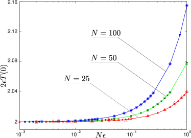
Figure 1: (Color online) Switching time as a function of $\epsilon$ for three different values of $N$. Empty symbols: Numerical simulation by a Gillespie algorithm over $10^{7}$paths ; filled symbols: numerical solution of the linear system (5-4); Solid lines: theoretical expression (7).

The analysis can be extended to compute the linear term in $\epsilon$ in equation (7) (see section V.A)

Equations (6,7) have been obtained by setting $r=1$, i.e. by scaling time and $\epsilon$ by the factor $r$. Restoring the non-scaled time ($t\rightarrow t/r$, $\epsilon\rightarrow\epsilon/r$), we have

$$\bar{T}_{\epsilon,r}^{(\mbox{ns)}}(0)=\frac{1}{r}\bar{T}_{\epsilon/r}(0)$$

and in particular, the leading terms of the development are

$$\bar{T}_{\epsilon,r}^{(\mbox{ns)}}(0)=\frac{1}{\epsilon}+\frac{2}{r}\frac{N-1}{N}+\frac{1}{r}O(\frac{\epsilon}{r})$$

Therefore, it is possible in principle, by measuring the switching time for different system size $N$, to measure independently the parameters $\epsilon$ and $r$.

Note that the rate coefficients used by Biancalani et al. are given in terms of proportions, i.e. $r^{\mbox{B}}=N^{2}r$ and $\epsilon^{\mbox{B}}=N\epsilon$. Figure 2 shows the comparison between our exact result and the Biancalani et al. approximate solutions when this scaling is taken into account, for the full range of $N\epsilon$. It can be observed that the two solutions obtained by Biancalani et al. and their overlap can be recovered from the exact solution we provide here.

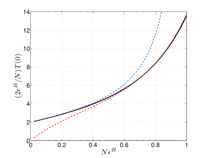
Figure 2: (Color online) Exact result for the first first passage time (solid line, black) as a function of $N$ for $\epsilon^{\mbox{B}}=1/500$, $r=1$ and its comparison to the two solutions provided by Biancalani et al.(Biancalani2014 , Figure 5) : dotted curve, blue for $\epsilon\rightarrow 0$ ; dotted curve, red for $N\epsilon^{\mbox{B}}\gtrsim 0.5$.

In a yet unpublished article, Saito and Kaneko Saito2014 have also computed the switching time for this stochastic system. Their method consists in obtaining an approximation for the residence time $t_{0,j}$ in each state $j$ beginning from state 0 and then summing up these residence times to obtain the switching time. Their analytical result for the switching time has a very different form that the relation (6) and doesn’t seem amenable to easy computation of the interesting limiting case $N\epsilon\ll 1$. However, their formula produces the same numerical results than the relation (6) of this article.

III Solving the master equation.

The mean first passage is one tool to study the stochastic system described by the transition rates (1,2). A complete description can be obtained by solving directly the master equation governing the probabilities $P(n,t)$ to observe $n$ individuals in state $A$ at time $t$:

$$\frac{\partial P(n,t)}{\partial t} = W^{+}(n-1)P(n-1,t)-W^{+}(n)P(n,t)$$ (8)

$$+ W^{-}(n+1)P(n+1,t)-W^{-}(n)P(n,t)$$

We note that the above stochastic system does not need a moment closure approximation, i.e. the equation for the $k$th moment involves only moments of order lower than $k$. Therefore, a hierarchical system of equations can be established to derive all the moments of this system. The probability generating function is a powerful tool to investigate such Master equations Gardiner2004 ; VanKampen1992 . The PGF is defined as

$$\phi(z,t)=\left\langle z^{n}\right\rangle=\sum_{n=0}^{N}P(n,t)z^{n}$$

and contains the most complete information we can have on the given stochastic process: all the moments and probabilities can be obtained from its derivatives at either $z=1$ or $z=0$. The equation governing the PGF can be extracted from the master equation (8) (see section V.3) and reads:

$$\frac{\partial\phi}{\partial t} = -z(z-1)^{2}\frac{\partial^{2}\phi}{\partial z^{2}}$$ (9)

$$+ (z-1)\left[\left(N-1-\epsilon\right)z-\left(N-1+\epsilon\right)\right]\frac{\partial\phi}{\partial z}$$

$$+ \epsilon N(z-1)\phi$$

The solution of equation (9) can be exactly computed (see section V.3) as the superposition of polynomial eigenfunctions

$$\phi(z,t)=\sum_{n=0}^{N}C_{n}\phi_{n}(z)e^{\lambda_{n}t}$$ (10)

where the eigenvalues are

$$\lambda_{n}=-n(n-1+2\epsilon),$$

the eigenfunctions are polynomials in $z$

$$\phi_{n}(z)=\sum_{k=n}^{N}a_{k}^{n}(1-z)^{k}$$

and the coefficients $C_{n}$ depend on the initial condition. The initial condition we use here is the same as in the previous section, $i.e.$ $P(n,0)=\delta_{n,0}$ which implies that $\phi(z,0)=1$. The exact expression for the coefficients $a_{k}^{n}$ , $C_{n}$ and their product are given in the section V.3. The agreement between the solution (10) and the direct numerical solution of the Master equation is displayed in figure 3.

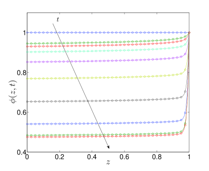
Figure 3: (Color online) The PGF function $\phi(z,t)$ as a function of $z$ at times $t\in\{0,1,2,4,8,16,32,64,128,256\}/(128\epsilon)$ for $N=100$ and $\epsilon=0.01$. Solid lines: theoretical expression (10). Circles: solution obtained by the numerical resolution of the Master equation (8) and computation of its PGF.

The PGF contains the most complete information on the stochastic process under investigation. Some quantities of interest extracted from it are given below.

III.1 Stationary probabilities.

The stationary probabilities attained at large times are

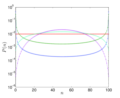
Figure 4: (Color online) The stationary probabilities $P(n,\infty)$ as a function of $n$ for $N=100$ and various $\epsilon$. Solid lines: exact expression (11), symbols: numerical resolution of the Master equation. $\epsilon=0.01$ (blue circles), $0.1$ (green squares), 1 (red diamonds), 2 (diamonds, cyan) and 4 ($\times$, purple).

$$P(n,\infty)=\binom{N}{n}\frac{(\epsilon)_{(n)}(\epsilon)_{(N-n)}}{(2\epsilon)_{(N)}}$$ (11)

(see section V.3) and their comparison to numerical solution of the Master equation is displayed in figure 4. Note the qualitative change of behavior at $\epsilon=1$. Expression (11) is equivalent to the expression found by Biancalani et al. Biancalani2014 in the continuous approximation, with the advantage of being well defined for all $n$, including $n=0,N$. In particular, for $\epsilon N\ll 1$,

$$P(n,\infty)\begin{cases}(1-H_{N-1}\epsilon)/2+O(\epsilon^{2})&n=0,N\\ \frac{N\epsilon}{2n(N-n)}+O(\epsilon^{2})&n\neq 0,N\end{cases}$$

where $H_{m}$ is the harmonic number $\sum_{i=1}^{m}i^{-1}$.

III.2 Factorial moments.

For the purposes of experimental measurements of the parameters, other dynamical quantities can be of interest. The most robust of these quantities are the factorial moments

$$\left\langle(n,q)\right\rangle=\left\langle n(n-1)...(n-q+1)\right\rangle$$

where $(n,q)$ is used to denote the decreasing Pochhammer symbol. The factorial moments are obtained by successive derivation of the PGF

$$\left\langle(n,q)\right\rangle =q! \left.\frac{\partial^{q}\phi}{\partial z^{q}}\right|_{z=1}$$ (12)

$$= (-1)^{q}q!\sum_{i=0}^{q}C_{i}a_{q}^{i}e^{\lambda_{i}t}$$

Note that the $q$th factorial moment involves only $q+1$ eigenfunctions. The two first factorial moments are

$$\left\langle n\right\rangle = \frac{N}{2}\left(1-e^{-2\epsilon t}\right)$$

$$\left\langle n(n-1)\right\rangle = \frac{N(N-1)}{2}$$

$$\times \left(\frac{1+\epsilon}{1+2\epsilon}-e^{-2\epsilon t}+\frac{\epsilon}{1+2\epsilon}e^{-2(1+2\epsilon)t}\right)$$

For $N\epsilon\ll 1$, only the two first terms in the sum (12) contribute significantly to the factorial moments for $t\gtrsim 1$. In particular, for large times,

$$\left\langle(n,q)\right\rangle\rightarrow(N,q)\frac{1-H_{q-1}\epsilon}{2}$$

III.3 Equilibrium time.

Finally, we can define an equilibrium time $T_{eq}$ by studying the dynamics of the decrease in $P(0,t)$ or increase in $P(N,t)$. The measure we choose to use here is

$$T_{eq}=\int_{0}^{\infty}\left\{P(N,\infty)-P(N,t)\right\}dt$$ (13)

which is a generalization of the mean first passage time (see V.3 ). The expressions for the two boundary probabilities are found to be

$$P(0,t) = \sum_{n=0}^{N}(-)^{N-n}C_{n}a_{N}^{n}e^{\lambda_{n}t}$$

$$P(N,t) = (-)^{N}\sum_{n=0}^{N}C_{n}a_{N}^{n}e^{\lambda_{n}t}$$

and therefore

$$T_{eq} = (-)^{N}\sum_{n=1}^{N}C_{n}a_{N}^{n}/\lambda_{n}$$ (14)

For $N\epsilon\lesssim 1$, eq.(14) is approximated by

$$T_{eq}=\frac{1}{4\epsilon}-\frac{1}{4}\left(H_{N-1}-2+\frac{2}{N}\right)$$ (15)

Figure 5 displays $T_{eq}$ as a function of $\epsilon$ and its comparison to numerical solution of the master equation.

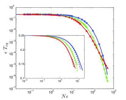
Figure 5: (Color online) $T_{eq}$ as a function of $\epsilon$ for different values of $N$. Solid lines: theoretical expression (14) ; symbols: numerical resolution of the master equation (blue circles $N=100$; green squares $N=50$ ; red triangles $N=25$). Inset: comparison between the exact expression (14) (solid lines) and its approximation (15)(dashed lines) for $N\epsilon\lesssim 1$ and $N=100,50$ and $25$.

IV Conclusion.

As discussed in the introduction, noise induced bi-stability has been intensely investigated, specially in genetic networks. In general, the chemical Master equations are too complex to be solved exactly and various approximation techniques have been developed to tackle this problem. In some cases, exact analytical solutions have been obtained using the probability generating function. Shahrezaei and Swain Shahrezaei2008 have studied a three stage model of simple gene expression (DNA state, RNA, Protein) and obtained the protein number distribution. Grima et al. Grima2012 have investigated the steady state distribution of a two component (DNA state, Protein) genetic feedback loop and have been able to obtain exact analytical results using the PGF technique. In the first case, the PGF equation is a first order partial differential equation and can be solved by the method of characteristics. In the second case, the model can be reduced to two coupled one component systems and the PGF equation reduced to two ordinary coupled first order differential equations. Chemical Master equations analogous to these cases could in principle be investigated with the same technique.

In this work, we have extended the investigation by Biancalani et al. Biancalani2014 of another noise induced bistable system which belongs to the second class of models discussed above. First, we have obtained the exact solution for the mean first passage time which is the main result of the above cited article. Second, we have solved the full master equation associated with this system and obtained other useful quantities for parameter estimations of such systems. We have obtained these results for the original, discrete system without resorting to the Taylor expansion of the Master equation in powers of $1/N$. Discrete solutions have the advantage of being clearly defined and avoid spurious effect happening at the boundaries, specially for the interesting case of small $\epsilon$. Moreover, these solutions involve only simple arithmetic and are easily computed.

V Mathematical details.

V.1 Series expansion of the exact solution of the switching time.

The exact solution (6) contains a double sum, where only the terms $i=0$ contain $\epsilon^{-1}$ factors. Separating these two contributions, the solution becomes:

$$\bar{T}(0) = \frac{1}{N\epsilon}\sum_{k=0}^{N-1}\frac{(1)_{k}}{(1+\epsilon)_{k}}\frac{(N-k+\epsilon)_{k}}{(N-k)_{k}}$$

$$+ \sum_{k=1}^{N-1}\sum_{i=1}^{k}\frac{(N-k+\epsilon)_{(k-i)}}{(N-k)_{(k-i+1)}}\frac{(i+1)_{(k-i)}}{(i+\epsilon)_{k-i+1}}$$

Expanding the first sum to the first order in $\epsilon$ necessitates only simple expansion in factors of the form $m/(m+\epsilon)=1-\epsilon/m+O(\epsilon^{2})$ and leads to

$$\frac{1}{\epsilon}-H_{N-1}+2\frac{N-1}{N}$$

where the Harmonic number $H_{m}=\sum_{i=1}^{m}(1/i)$. Evaluating the second sum for $\epsilon=0$ results in

$$\sum_{k=1}^{N-1}\sum_{i=1}^{k}\frac{1}{i(N-i)}=H_{N-1}$$

Adding the two contributions results in (eq.7):

$$\bar{T}(0)=\frac{1}{\epsilon}+2\frac{N-1}{N}$$

The next term in the series expansion of $\bar{T}(0)$ is found to be

$$-\frac{2\epsilon}{N}\left(H_{N-1}+NH_{N-1}^{(2)}-2(N-1)\right)$$

Note that algorithmically, the computation of $\bar{T}(0)$ (expression (6) ) necessitates only the calculation of $N$ ratios of the form $(m+1)/(m+\epsilon)$ and $(m+\epsilon)/m$ which can be stored in an array. The $\bar{T}(0$) involves then only multiplications and sums of these elements. The Hypergeometric function on the other hand is defined as

$${}_{2}F_{1}(a,b;c;z)=\sum_{n=0}^{\infty}\frac{(a)_{(n)}(b)_{(n)}}{(c)_{(n)}}\frac{z^{n}}{n!}$$

and its efficient implementation requires specific algorithms.

V.2 Solution of Biancalani et al. for the switching time.

In non scaled time, the Biancalani et al. solution is

$$\bar{T}^{\mbox{ns}}(0) = \frac{1}{r^{\prime}}\frac{2N^{2}}{1+2\epsilon^{\prime}/r^{\prime}}\,_{2}F_{1}\left(\frac{1}{2},1-N\frac{\epsilon^{\prime}}{r^{\prime}};\frac{3}{2};\frac{1}{1+2\epsilon^{\prime}/r^{\prime}}\right)$$

$$\times \,{}_{2}F_{1}\left(\frac{1}{2},N\frac{\epsilon^{\prime}}{r^{\prime}};\frac{3}{2};\frac{1}{1+2\epsilon^{\prime}/r^{\prime}}\right)$$

where the rates $\epsilon^{\prime}$ and $r^{\prime}$ are related to the rates $\epsilon$,$r$ used in this article through:

$$\epsilon^{\prime}=N\epsilon\,\,;\,\,r^{\prime}=N^{2}r$$

V.3 Deriving and solving the PGF equation.

PGF.

The equation for the evolution of the PGF is obtained by multiplying the master equation(8) by $z^{n}$ and summing over $n$ Houchmandzadeh2010 . This operation leads to

$$\frac{\partial\phi}{\partial t}=\left\langle(z^{n+1}-z^{n})W^{+}(n)\right\rangle+\left\langle(z^{n-1}-z^{n})W^{-}(n)\right\rangle$$ (16)

The rates $W^{\pm}(n)$ are polynomials of second degree in $n$ and by the definition of the PGF,

$$\left\langle n^{r}z^{n}\right\rangle=\left(z\frac{\partial}{\partial z}\right)^{r}\phi$$

Application of the above rule to equation (16) leads to equation (9).

Eigenfunctions.

Equation (9) can be transformed into a hypergeometric equation by a change of variable $x=(z-1)^{-1}$. It is however much simpler to use the fact that by definition, the function $\phi(z,t)$ is a polynomial of degree $N$ in $z$ and search for the eigenfunctions of equation (9) in term of polynomials of the following form:

$$\phi_{n}(z)=\sum_{k=0}^{N}a_{k}^{n}(1-z)^{k}$$

i.e.

$$\phi(z,t)=\sum_{n=0}^{N}C_{n}\phi_{n}(z)e^{\lambda_{n}t}$$

Insertion of these polynomials into equation (9) shows that non-trivial solutions (i.e. $\neq 0$) are possible only for the eigenvalues

$$\lambda_{n}=-n(n-1+2\epsilon)\,\,\,\,n=0,1,...,N$$

which leads to a one term recurrence relation on the coefficients $a_{k}^{n}$ :

$$a_{k}^{n} = 0\,\,\,\,\,\,(k<n)$$

$$a_{n}^{n} = 1$$

$$a_{k+1}^{n} = -\frac{(N-k)(k+\epsilon)}{(k+1)(k+2\epsilon)-n(n-1+2\epsilon)}a_{k}^{n}\,\,\,\,\,\,(n\leq k<N)$$

As it can be noticed, $\phi_{n}$ is written as polynomial in powers of $(1-z)$ and not $z$. This choice is not arbitrary: it is this change of variable which allows to obtain a one term recurrence relation between the coefficients $a_{k}^{n}$. Writing $\phi_{n}$ as a polynomial in $z$ leads to a two terms recurrence relation which is much more intricate to solve exactly.

The coefficients $a_{k}^{n}$ can be computed in explicit forms:

$$a_{k}^{n}=(-)^{k-n}\binom{N-n}{k-n}\frac{(\epsilon+n)_{(k-n)}}{(2\epsilon+2n)_{(k-n)}}\,\,\,\,\,\,(n\leq k<N)$$ (17)

Alternatively, the eigenfunctions can also be given in terms of the hypergeometric function:

$$\phi_{n}(z)=(1-z)^{n}\,\,_{2}F_{1}(n-N,n+\epsilon;2n+2\epsilon;1-z)$$ (18)

The amplitudes $C_{n}$ depend on the initial condition. For $P(n,0)=\delta_{n,0}$ and therefore $\phi(z,0)=1$, the amplitudes obey the triangular linear system

$$C_{0} = 1$$

$$\sum_{n=0}^{k}C_{n}a_{k}^{n} = 0\,\,\,\,(k>0)$$

which can be explicitly solved

$$C_{n}=\left(\begin{array}[]{c}N\\ n\end{array}\right)\frac{(\epsilon)_{(n)}}{(2\epsilon+n-1)_{(n)}}$$ (19)

and therefore,

$$C_{n}a_{k}^{n}=(-)^{k-n}\binom{N}{k}\binom{k}{n}\frac{(\epsilon)_{(k)}}{(2\epsilon+n)_{(k)}}\frac{2\epsilon+2n-1}{2\epsilon+n-1}$$

Stationary probabilities.

As all eigenvalues except $\lambda_{0}$ are negative, for large times the PGF is simply

$$\phi(z)={}_{2}F_{1}(-N,\epsilon;2\epsilon;1-z)$$

where we have used the hypergeometric representation (eq. 18) of the eigenfunctions. Using the relations

$${}_{2}F_{1}(-m,b;c;1) = \frac{(c-b)_{(m)}}{(c)_{(m)}}$$

$$\frac{d^{n}}{dz^{n}}\,_{2}F_{1}(a,b;c;z) = \frac{(a)_{(n)}(b)_{(n)}}{(c)_{(n)}}\,_{2}F_{1}(a+n,b+n;c+n;z)$$

we obtain

$$P(n) = \frac{1}{n!}\left.\frac{d^{n}\phi}{dz^{n}}\right|_{z=0}$$ (20)

$$= (-1)^{n}\frac{(-N)_{(n)}}{n!}\frac{(\epsilon)_{(n)}}{(2\epsilon)_{(n)}}\frac{(\epsilon)_{(N-n)}}{(2\epsilon+n)_{(N-n)}}$$

As

$$(2\epsilon)_{(n)}(2\epsilon+n)_{(N-n)}=(2\epsilon)_{N}$$

we recover the relation (11) on the stationary probabilities.

Factorial moments.

Using the above expression, the factorial moments are

$$\left\langle(n,q)\right\rangle=(N,q)\sum_{i=0}^{q}(-)^{i}\binom{q}{i}\frac{(\epsilon)_{(q)}}{(2\epsilon+i)_{(q)}}\frac{2\epsilon+2i-1}{2\epsilon+i-1}e^{\lambda_{i}t}$$

Equilibrium times.

Many different measures can be used for the equilibrium time of the system. The expression we use

$$T_{eq}=\int_{0}^{\infty}\left(P(N,\infty)-P(N,t)\right)dt$$ (21)

is the extension of the mean time to absorption to the case when the boundary state is not absorbing. The reason is the following: If the state $N$ were the only absorbing state, whatever the initial condition $m$, $P(N,t)\rightarrow 1$ as $t\rightarrow\infty$. The probability of survival until time $T$, beginning in the state $m$ is

$$Q(m,T)=1-P(N,T)$$

and the probability density of not being absorbed during $[T,T+dt]$ is therefore $-\partial_{T}Q(m,T)$. Therefore, the mean time to absorption is

$$\bar{T}(m) = -\int_{0}^{\infty}T\partial_{T}Q(m,T)dT$$

$$= \int_{0}^{\infty}\left(1-P(N,T)\right)dT$$

$$= \int_{0}^{\infty}\left(P(N,\infty)-P(N,T)\right)dT$$

We see that in the case of an absorbing state $N$, our definition of $T_{eq}$ and the mean time to absorption are the same. We continue to use $T_{eq}$ as a measure of the equilibrium time when $N$ is not absorbing.

Probabilities.

The probabilities are extracted from the PGF by collecting the coefficients of powers of $z$:

$$P(n,t)=\sum_{k=0}^{N}b_{k}^{n}\exp(\lambda_{k}t)$$

where

$$b_{k}^{n}=(-)^{n}C_{k}\sum_{j=k}^{N}\left(\begin{array}[]{c}j\\ n\end{array}\right)a_{j}^{k}.$$

References

- [1] José M G Vilar, Hao Yuan Kueh, Naama Barkai, and Stanislas Leibler. Mechanisms of noise-resistance in genetic oscillators. Proceedings of the National Academy of Sciences of the United States of America, 99(9):5988–92, April 2002.
- [2] Bahram Houchmandzadeh and Marcel Vallade. Selection for altruism through random drift in variable size populations. BMC Evol Biol, 12:61, 2012.
- [3] K S Korolev, Mikkel Avlund, Oskar Hallatschek, and David R Nelson. Genetic demixing and evolution in linear stepping stone models. Reviews of modern physics, 82(2):1691–1718, June 2010.
- [4] B Houchmandzadeh. Neutral clustering in a simple experimental ecological community. Phys Rev Lett, 101(7):78103, 2008.
- [5] Eric Dumonteil, Fausto Malvagi, Andrea Zoia, Alain Mazzolo, Davide Artusio, Cyril Dieudonné, and Clélia De Mulatier. Particle clustering in Monte Carlo criticality simulations. Annals of Nuclear Energy, 63:612–618, January 2014.
- [6] W. Horsthemke and R. Lefeve. Noise-Induced Transitions: Theory and Applications in Physics, Chemistry, and Biology. Springer-Verlag, Berlin, 1986.
- [7] Michael Samoilov, Sergey Plyasunov, and Adam P Arkin. Stochastic amplification and signaling in enzymatic futile cycles through noise-induced bistability with oscillations. Proceedings of the National Academy of Sciences of the United States of America, 102(7):2310–5, February 2005.
- [8] Maxim N Artyomov, Jayajit Das, Mehran Kardar, and Arup K Chakraborty. Purely stochastic binary decisions in cell signaling models without underlying deterministic bistabilities. Proceedings of the National Academy of Sciences of the United States of America, 104(48):18958–63, November 2007.
- [9] Hong Qian, Pei-Zhe Shi, and Jianhua Xing. Stochastic bifurcation, slow fluctuations, and bistability as an origin of biochemical complexity. Physical chemistry chemical physics : PCCP, 11(24):4861–70, June 2009.
- [10] Philipp Thomas, Nikola Popović, and Ramon Grima. Phenotypic switching in gene regulatory networks. Proceedings of the National Academy of Sciences of the United States of America, 111(19):6994–9, May 2014.
- [11] Tsz-Leung To and Narendra Maheshri. Noise can induce bimodality in positive transcriptional feedback loops without bistability. Science (New York, N.Y.), 327(5969):1142–5, February 2010.
- [12] Tommaso Biancalani, Louise Dyson, and Alan J. McKane. Noise-Induced Bistable States and Their Mean Switching Time in Foraging Colonies. Physical Review Letters, 112(3):038101, January 2014.
- [13] P A P Moran. The Statistical processes of of evolutionary theory. Oxford University Press, 1962.
- [14] Yuichi Togashi and Kunihiko Kaneko. Transitions Induced by the Discreteness of Molecules in a Small Autocatalytic System. Physical Review Letters, 86(11):2459–2462, March 2001.
- [15] Jun Ohkubo, Nadav Shnerb, and David A. Kessler. Transition Phenomena Induced by Internal Noise and Quasi-Absorbing State. Journal of the Physical Society of Japan, 77(4):044002, April 2008.
- [16] Tommaso Biancalani, Tim Rogers, and Alan J. McKane. Noise-induced metastability in biochemical networks. Physical Review E, 86(1):010106, July 2012.
- [17] Roy J. Glauber. Time-Dependent Statistics of the Ising Model. Journal of Mathematical Physics, 4(2):294, December 1963.
- [18] C Gardiner. Handbook of Stochastic Methods: for Physics, Chemistry and the Natural Sciences. Springer, 2004.
- [19] Nen Saito and Kunihiko Kaneko. Theoretical Analysis of Discreteness-Induced Transition in Autocatalytic Reaction Dynamics. arXiv:1403, March 2014.
- [20] N G Van Kampen. Stochastic processes in physics and chemistry, volume 11. North- Holland personal library, 1992.
- [21] Vahid Shahrezaei and Peter S Swain. Analytical distributions for stochastic gene expression. Proceedings of the National Academy of Sciences of the United States of America, 105(45):17256–61, November 2008.
- [22] R Grima, D R Schmidt, and T J Newman. Steady-state fluctuations of a genetic feedback loop: an exact solution. The Journal of chemical physics, 137(3):035104, July 2012.
- [23] B Houchmandzadeh and M Vallade. Alternative to the diffusion equation in population genetics. Phys Rev E Stat Nonlin Soft Matter Phys, 82(5 Pt 1):51913, 2010.