NRCPS-HE-1-2015
SigmaPhi2014, July 2014
Rhodes , Greece

The Gonihedric Paradigm
Extensions of the Ising Model

George Savvidy

Institute of Nuclear and Particle Physics

Demokritos National Research Center

Ag. Paraskevi, Athens, Greece

Abstract

We suggest a generalization of the Feynman path integral to an integral over random surfaces. The proposed action is proportional to the linear size of the random surfaces and is called gonihedric. The convergence and the properties of the partition function are analysed. The model can also be formulated as a spin system with identical partition function. The spin system represents a generalisation of the Ising model with ferromagnetic, antiferromagnetic and quartic interactions. Higher symmetry of the model allows to construct dual spin systems in three and four dimensions. In three dimensions the transfer matrix describes the propagation of closed loops and we found its exact spectrum. It is a unique exact solution of the tree-dimensional statistical spin system. In three and four dimensions the system exhibits the second order phase transitions. The gonihedric spin systems have exponentially degenerated vacuum states separated by the potential barriers and can be used as a storage of binary information.

1 Extension of Feynman Path Integral

Feynman path integral over trajectories describes quantum-mechanical behaviour of point-like particles, and it is an important problem to extend the path integral to an integral which describes a quantum-mechanical motion of strings. A string is a one dimensional extended object which moves through the space-time. As string moves through the space-time it sweeps out a two-dimensional surface, and in order to describe its quantum-mechanical behavior one should define an appropriate action and the corresponding functional integral over two-dimensional surfaces.

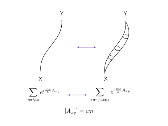
Figure 1: On the left hand side of the figure there is a trajectory of a structureless point particle with an action which is proportional to the length of its world line. On the right there is a world sheet surface which is swept by a propagating closed string. It is required that the string action $A_{xy}$ should be proportional to the linear size of the space-time surface, measuring it in terms of its length, similar to the action of a point-like particle. This is a natural requirement because when a string collapses to a point its world sheet will degenerate into a world line and both actions will coincide.

In string theory the action is defined by using Nambu-Goto area action [1, 2]. The area action suffers from spike instabilities [3], because the zero-area spikes can easily grow on a surface. Indeed, the spikes have zero area, and there is no suppression of the spike fluctuations in the functional integral. Different modifications of the area action have been suggested in the literature to cure these instabilities, which are based on the addition of extrinsic curvature terms [4] to the area action.

Figure 2: On the left there is a discrete trajectory with an action which is proportional to the sum of the lengths of its edges. On the right there is a discretized surface and the action is a sum of the lengths of its edges multiplied by the corresponding deficit angles.

The alternative principle to cure surface instabilities was put forward in [5, 6, 7]. In its essence there is a new requirement which should be imposed on the string action. The string action should be defined in such a way that when a string shrinks to a point-like object its action should reduce to an action of point-like particle [5]. In other words, when a surface shrinks to a space-time curve, its action should reduce to the length of the curve (see Fig. 1 ). It is almost obvious that now the spikes cannot easily grow on a surface because in the functional integral such fluctuations will be suppressed exponentially $e^{-m\lambda_{spike}}$, where $\lambda_{spike}$ is the length of the spike.

One can consider smooth surfaces, as well as discretized random surfaces which are represented by polyhedral surfaces build from triangles (see Fig. 2). For smooth surfaces the proposed action has the form [8, 9, 10, 11, 12]

$$A(M)=m\int d^{2}\zeta\sqrt{g}\sqrt{\left(\Delta(g)X^{\mu}\right)^{2}}~{}~{}~{}~{}\rightarrow~{}~{}~{}~{}m\int ds,$$ (1.1)

where $g_{ab}=\partial_{a}X^{\mu}\partial_{b}X^{\mu}$ is the induced metric and $\Delta(g)$ is a Laplace operator. For discretized surfaces the action is defined as a sum over links and deficit angles [5, 6, 7]:

$$A(M)=m\sum_{<ij>}\lambda_{ij}|\pi-\alpha_{ij}|~{}~{}~{}~{}~{}\rightarrow~{}~{}~{}~{}~{}~{}~{}~{}~{}m\sum_{<ij>}\lambda_{ij}.$$ (1.2)

The action involves the products of edge length $\lambda_{ij}=|x_{i}-x_{j}|$ times the corresponding deficit angle $|\pi-\alpha_{ij}|$, and it was suggested to call that action - gonihedric from two hellenic words $\gamma\omega\nu\iota^{\prime}\alpha$ - the angle and $\epsilon^{\prime}\delta\rho\alpha$ - the side. The corresponding partition function can be represented in the form

$$Z(\beta)=\sum_{N}\int d^{D}x_{1}....d^{D}x_{N}\exp{(-\beta m\sum_{<ij>}|x_{i}-x_{j}||\pi-\alpha_{ij}|)}.$$ (1.3)

The general arguments, based on the Minkowski inequality [5], show that the maximal contribution to the partition function comes from the surfaces close to a sphere. The convergence of the partition function was proven rigorously in [13, 14, 15] . Because the action is proportional to the ”perimeter” of the surface, and not to its area, the classical string tension is equal to zero and the model can equally well be called a model of tensionless strings [8, 9, 10, 11].

It is important to study the phase structure of the system (1.3) in order to identify quantum field theory to which it is equivalent near its critical point [25, 26, 27]. At low temperature the Wegner-Wilson loop correlation functions have perimeter behavior. At high temperature the fluctuations of the surface induce the area behavior signaling that there is a confinement - deconfinement (or area - perimeter) phase transition [5, 6, 8]. In this model a nonzero string tension is entirely generated by quantum (thermodynamical) fluctuations [6, 8, 7].

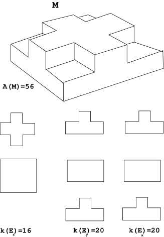
Figure 3: On the top is an example of a surface M on hyper cubic lattice. The set of planes $\{E_{x}\},\{E_{y}\},\{E_{z}\}$ perpendicular to $x,y,z$ axis intersect a given surface $M$ in the middle of the links. On each of these planes we shall have an image of the surface $M$. Every such image is represented by closed polygon-loops $P(E)$ appearing in the intersection of the plane with surface $M$. The energy of the surface $M$ is equal to the sum of the total curvature $k(E)$ on all these planes, as it is given by the formula (4.17). For the surface on the picture this sum is equal to $A(M)=16+20+20=56$ times $a{\pi\over 2}$. As we shall see, the energy of the surface M can be recovered by using images of the surface only on one sequence of parallel planes (4.21). On Fig. 4 this is demonstrated by using only images of the surface M on $\{E_{z}\}$ planes.

2 Extensions of the Ising and Wegner Models

The model of gonihedric random surfaces was formulated as embedding of random surfaces into the Euclidean space [5, 6, 7]. It can also be formulated as a model of random surfaces embedded into the hyper-cubic lattice [16, 17, 18, 19, 20] (see Fig.  3). The advantage of the lattice formulation consists in the fact that one can construct a spin system which is a generalisation of the Ising model with ferromagnetic, antiferromagnetic and quartic interactions so that its interface energy is equal to the gonihedric energy (1.2).

On the lattice a closed surface $M$ can be considered as a collection of plaquettes the edges of which are glued together pairwise. The surface is considered as a connected, orientable surface with given topology, and it is assumed that self-intersections of the surface produce additional contributions to the energy functional proportional to the length of the intersections. On the lattice the lengths of the elementary edges $\lambda_{ij}=|x_{i}-x_{j}|$ are equal to the lattice constant $a$ and the angles between plaquettes are either $0$ or $\pi/2$. The gonihedric energy functional (1.2) on the hyper-cubic lattice therefore takes the following form:

$$A(M)=(n_{2}+4kn_{4})~{}a~{}{\pi\over 2}$$ (2.4)

where $n_{2}$ is the total number of edges on which two plaquettes intersect at right angle, $n_{4}$ is the total number of edges with four intersecting plaquettes and $k$ is the self-intersection coupling constant. It describes the intensity of string interactions: string can split into two strings and merge with other strings (see Fig. 7). The equivalent Hamiltonian of the spin system on three-dimensional lattice has the form [16, 17, 18]

$$H^{3d}_{gonihedric}=-2k\sum_{\vec{r},\vec{\alpha}}\sigma_{\vec{r}}\sigma_{\vec{r}+\vec{\alpha}}+\frac{k}{2}\sum_{\vec{r},\vec{\alpha},\vec{\beta}}\sigma_{\vec{r}}\sigma_{\vec{r}+\vec{\alpha}+\vec{\beta}}-\frac{1-k}{2}\sum_{\vec{r},\vec{\alpha},\vec{\beta}}\sigma_{\vec{r}}\sigma_{\vec{r}+\vec{\alpha}}\sigma_{\vec{r}+\vec{\alpha}+\vec{\beta}}\sigma_{\vec{r}+\vec{\beta}},$$ (2.5)

where the vector $\vec{\alpha}$ runs over the unit vectors parallel to the axes. Similarly, the sum over $\vec{\alpha}$ and $\vec{\beta}$ runs over different pairs of such vectors. The Hamiltonian represents a magnetic system with competing interaction and specially adjusted coupling constants $J_{ferr}=4J_{antiferr}=2k$. The Hamiltonian (2.5) contains the usual Ising ferromagnet

$$H_{Ising}^{3d}=-J\sum_{\vec{r},\vec{\alpha}}\sigma_{\vec{r}}\sigma_{\vec{r}+\vec{\alpha}}$$

with additional diagonal antiferromagnetic interaction and quartic spin interaction which regulates the intensity of the interaction at the self-intersection edges. When $k=0$ the surfaces can freely intersect, at $k=\infty$ the surfaces are strongly self-avoiding [17, 18].

The partition functions of both systems (2.4) and (2.5) are identical to each other:

$$Z(\beta)=\sum_{\{M\}}e^{-\beta~{}A(M)}~{}=~{}\sum_{\{\sigma\}}e^{-\beta H_{gonihedric}(\sigma)}.$$ (2.6)

In the first case it is a sum over all two-dimensional surfaces of the type described above with energy functional $A(M)$, in the second case it is a sum over all spin configurations. This spin system has very high symmetry because one can flip the spins on any flat hypersurface without changing the energy of the system. The rate of degeneracy of the vacuum state depends on the self-intersection coupling constant $k$ [18, 19]. If $k\neq 0$, the degeneracy of the vacuum state is equal to $3\cdot 2^{N}$ for the lattice of the size $N^{3}$, because one can flip spins on any set of parallel planes [18, 19] .

A similar construction can be performed in four dimensions [16, 17]. On a four-dimensional lattice a two-dimensional closed surface can have self-intersections of different orders because at a given edge one can have self-intersections of four or six plaquttes. The energy which is ascribed to self-intersections essentially depends on a configuration of plaquettes in the intersection. There are two topologically different configurations of plaquettes with four intersecting plaquettes and only one with six intersecting plaquettes. The corresponding spin system is locally gauge invariant [17]:

$$H^{4d}_{gonihedric}=-\frac{5\kappa-1}{g^{2}}\sum_{\{plaq\}}(\sigma\sigma\sigma\sigma)+\frac{\kappa}{4g^{2}}\sum_{\{right~{}angle~{}plaq\}}(\sigma\sigma\sigma\sigma_{\alpha})^{rt}(\sigma_{\alpha}\sigma\sigma\sigma)$$

$$-\frac{1-\kappa}{8g^{2}}\sum_{\{triples~{}of~{}right~{}angle~{}plaq\}}(\sigma\sigma\sigma\sigma_{\alpha})^{rt}(\sigma_{\alpha}\sigma\sigma\sigma_{\beta})^{rt}(\sigma_{\beta}\sigma\sigma\sigma).$$ (2.7)

The total energy of the surface in this case is

$$A(M)=(n_{2}+4k\bar{n}_{4}+(6k-1)\bar{\bar{n}}_{4}+12kn_{6})~{}a~{}{\pi\over 2},$$ (2.8)

where $n_{2}$ is the total number of edges, where two plaquettes intersect at the right angle, $\bar{n}_{4}$ and $\bar{\bar{n}}_{4}$ edges with intersection of four plaquettes and $n_{6}$ with six plaquettes. The partition functions of both four-dimensional systems (2) and (2.8) are identical to each other, as in (2.6). Thus a sum over all two-dimensional surfaces of the type described above with energy functional $A(M)$, embedded into a four-dimensional lattice is identical to a sum over all spin configurations.

The spin systems described above can be studied by powerful analytical methods [19, 20, 21, 22, 29, 30, 31], as well as by Monte-Carlo simulations [36, 37, 38, 39, 41].

Figure 4: The energy of the surface M can be recovered by using images of the surface only on one sequence of the parallel planes (4.21). For the surface on the picture we have $k(P_{1})=4,k(P_{2})=12,l(\emptyset\bigtriangleup P_{1})=12,l(P_{1}\bigtriangleup P_{2})=16,l(P_{2}\bigtriangleup\emptyset)=12$. Here $\emptyset$ denotes an empty polygon and $\bigtriangleup$ a symmetric difference (4.20). Summing all these quantities in accordance with the formula (4.21) we shall get $A(M)=4+12+12+16+12=56$ times $a{\pi\over 2}$. This, as it should, coincides with the previous result on Fig. 3. With the use of this representation the transfer martix (4.23) can be viewed as describing the propagation of the polygon-loop $P_{1}$ at time $\tau$ to another polygon-loop $P_{2}$ at the time $\tau+1$.

3 Dual Spin Systems

Of a special interest is a system with self-intersection coupling constant equal to zero, $k=0$ [18, 19]. Because in that case the surfaces can freely self-intersect, the system has even higher symmetry: one can flip spins $\sigma\rightarrow-\sigma$ on any set of planes orthogonal to the axis $x,y,z$. In this limit the Hamiltonian (2.5) reduces to the following form: [18, 19]

$$H_{gonihedric}^{3d}=-\frac{1}{2}\sum_{\vec{r},\vec{\alpha},\vec{\beta}}\sigma_{\vec{r}}\sigma_{\vec{r}+\vec{\alpha}}\sigma_{\vec{r}+\vec{\alpha}+\vec{\beta}}\sigma_{\vec{r}+\vec{\beta}}$$ (3.9)

and its vacuum state degeneracy increases and is equal to $2^{3N}$ [18, 19]. The last case is a sort of ”supersymmetric” point in the space of gonihedric Hamiltonians (2.5).

It is well known that the two-dimensional Ising model is a sef-dual system and that three-dimensional Ising model is dual to the gauge spin system[23]. This duality was an important fact allowing to find the exact solution of the Ising model in two dimensions. We were able to construct dual systems for the gonihedric spin systems in three and four dimensions [19, 20]. In three dimensions the dual spin system is of the form[19]

$$H^{3d}_{dual}=-\sum_{\xi}R^{\chi}(\xi)\cdot R^{\chi}(\xi+\chi)+R^{\eta}(\xi)\cdot R^{\eta}(\xi+\eta)+R^{\varsigma}(\xi)\cdot R^{\varsigma}(\xi+\varsigma),$$ (3.10)

where $\chi$, $\eta$ and $\varsigma$ are unit vectors in the orthogonal directions of the dual lattice and $R^{\chi}$, $R^{\eta}$ and $R^{\varsigma}$ are one-dimensional irreducible representations of the group $Z_{2}\times Z_{2}$.

Similar construction can be performed in four dimensions [20]. But, unlike the three-dimensional case, where we set the self-intersection coupling constant $k$ to be equal to zero in (2), here appears a complication. Indeed, if in four dimensions we set the self-intersection coupling constant $k$ to be equal to zero then the Hamiltonian (2) has one and three plaquette terms and if we take $k=1$, then it has one and two plaquette terms. In order to have even high symmetry one can choose special weights on the intersections. Consider the case when the intersection of six plaquettes contributes zero energy so that it can be uniquely decomposed into three flat pairs of plaquettes. The intersection of four plaquettes yields zero energy in the cases when the plaquettes lie on two flat planes and with the energy equal to $a\pi/2$ if a pair of plaquettes is left out of a plane. Therefore a four-plaquette intersection also uniquely decomposes into two flat planes in the first case and into one flat plane and one ”corner” in the second case. For this choice of the self-intersection energies the Hamiltonian has the form [20]

$$H^{4d}_{gonihedric}=-\sum_{pairs~{}of~{}parallel~{}plaq}(\sigma\sigma\sigma\sigma)_{P}^{~{}~{}||}(\sigma\sigma\sigma\sigma)_{P},$$ (3.11)

where the summation is extended over all pairs of parallel plaquettes in $3d$ cubes of the $4d$ lattice. Here the Ising spins $\sigma_{\vec{r},\vec{r}+\vec{\alpha}}$ are located in the center of the links $(\vec{r},\vec{r}+\vec{\alpha})$ of the four-dimensional lattice. One can check that the low temperature expansion of the partition function of this system,

$$Z(\beta)=\sum_{\{\sigma\}}e^{-\beta H^{4d}_{gonihedric}}=~{}\sum_{\{M\}}e^{-\beta A(M)},$$ (3.12)

is obtained by summation over all closed surfaces $\{M\}$ with the weight $e^{-\beta A(M)}$, where the linear action $A(M)$ is given by the number of non-flat pairs of plaquettes of the closed surface $M$.

The details of the construction of the dual Hamiltonian can be found in [20]. Here we shall present its final form [20]:

$$H^{4d}_{dual}=-\sum_{\xi}\sum_{\nu\neq\mu}\Lambda_{\nu,\mu}(\xi)\cdot\Gamma(\xi,\xi+e_{\mu})\cdot\Lambda_{\mu,\nu}(\xi+e_{\mu}).$$ (3.13)

It is a spin system of six Ising spins $\Lambda_{\mu,\nu}(\xi)=\Lambda_{\nu,\mu}(\xi)$, $\mu\neq\nu=1,2,3,4$ located on every $vertex$ $\xi$ of the lattice and of one Ising spin $\Gamma(\xi,\xi+e_{\mu})$ located on the center of every $link$ $(\xi,\xi+e_{\mu})$, where $e_{\mu}$ are the unite vectors along the four axis.

Both Hamiltonian (3.10) and (3.13) look differently, but it is possible to rederive (3.10) in the form which is similar to (3.13). For that let us introduce three different Ising spins $\{\Lambda_{1},\Lambda_{2},\Lambda_{3}\}$ in every vertex $\xi$, then

$$H^{3d}_{dual}=\sum_{i\neq j\neq k}\Lambda_{j}(\xi)\Lambda_{k}(\xi)\Lambda_{j}(\xi+e_{i})\Lambda_{k}(\xi+e_{i}).$$ (3.14)

As we shall see in the next section, this approach allows to construct the corresponding transfer matrix, to prove that it describes the propagation of closed loops and in a special case to find its spectrum. This will present a unique exact solution of the tree-dimensional statistical spin system.

4 Transfer Matrices and Exact Solutions

Figure 5: Intersection of the polyhedral surface $M$ by the plane $E$. The image of the surface on the plane is a polygon $P$ and its curvature is equal to $k(E)$.

In this section we shall consider the above model of random surfaces embedded into 3d Euclidean lattice $Z^{3}$. The reason to focus on this particular case is motivated by the fact that one can geometrically construct the corresponding transfer matrix [29] and find its exact spectrum [30, 31, 32].

In order to find transfer matrix for this system we have to use the Geometrical theorem proven in [13]. The geometrical theorem provides an equivalent representation of the action $A(M)$ in terms of the absolute total curvature $k(E)$ of the polygon $P(E)$ which appears in the intersection of the two-dimensional plane $E$ with the given two-dimensional surface $M$ (see Fig. 5):

$$k(E)=\sum_{<i,j>}|\pi-\alpha^{E}_{ij}|,$$ (4.15)

where $\alpha^{E}_{ij}$ are the angles of this polygon. They are defined as the angles in the intersection of the two-dimensional plane $E$ with the edge $<ij>$ (see Fig. 5). The meaning of (4.15) is that it measures the total revolution of the tangent vectors to polygon $P_{E}$. By integrating the total curvature $k(E)$ in (4.15) over all intersecting planes $E$ we shall get the action $A(M)$ [13]:

$$A(M)=\frac{1}{2\pi}\int_{\{E\}}k(E)dE.$$ (4.16)

Geometrical Theorem on a lattice [17, 18, 19]. One can find the same representation (4.16) for the action $A(M)$ on a cubic lattice $Z^{3}$ by introducing a set of planes $\{E_{x}\},\{E_{y}\},\{E_{z}\}$ perpendicular to $x,y,z$ axis on the dual lattice. These planes will intersect a given surface $M$ and on each of these planes we shall have an image of the surface $M$. Every such image is represented as a collection of closed polygons $Q(E)$ appearing in the intersection of the plane with surface $M$ (see Fig. 3,4). The energy of the surface $M$ is equal now to the sum of the total curvature $k(E)$ of all these polygons on different planes:

$$A(M)=\sum_{\{E_{x},E_{y},E_{z}\}}k(E).$$ (4.17)

The total curvature $k(E)$ is the total number of polygon right angles. With (4.17) the partition function of the system (2.6) can be written in the form

$$Z(\beta)=\sum_{\{M\}}\exp\{-2\beta\sum_{\{E\}}k(E)\},$$ (4.18)

where the sum in the exponent can be represented as a product:

$$\prod_{\{E\}}e^{-2\beta k(E)}=\prod_{\{E_{z}\}}e^{-2\beta k(E_{z})}\prod_{\{E_{y}\}}e^{-2\beta k(E_{y})}\prod_{\{E_{x}\}}e^{-2\beta k(E_{x})}.$$ (4.19)

The goal is to express the energy functional (4.17) and the product (4.19) in terms of images on parallel planes in one fixed direction, let us say, $\{E_{z}\}$. The question is: what kind of information do we need to know on planes $\{E_{z}\}$ in order to recover the values of the total curvature $k(E_{x})$ and $k(E_{y})$ on the planes $\{E_{y}\}$ and $\{E_{x}\}$? The contribution to the curvature $k(E_{x})+k(E_{y})$ of the polygons which are on the perpendicular planes between $E^{i}_{z}$ and $E^{i+1}_{z}$ is equal to the length of the polygons $Q_{i}$ and $Q_{i+1}$ without length of the common bonds:

$$l(Q_{i})+l(Q_{i+1})-2\cdot l(Q_{i}\cap Q_{i+1})=l(Q_{i}\bigtriangleup Q_{i+1}),$$ (4.20)

where the polygon-loop  $Q_{1}\bigtriangleup Q_{2}~{}\equiv~{}Q_{1}\cup Q_{2}~{}\backslash~{}Q_{1}\cap Q_{2}$  is a union $Q_{1}\cup Q_{2}$ without intersection $Q_{1}\cap Q_{2}$. Therefore the energy (4.17) can be expressed by using images only on $\{E_{z}\}$ planes:

$$A(M)=\sum_{\{E\}}k(E)=\sum_{\{E_{z}\}}k(Q_{i})+l(Q_{i}\bigtriangleup Q_{i+1}).$$ (4.21)

The partition function (4.18) can be now represented in the form

$$Z(\beta)=\sum_{\{Q_{1},Q_{2},...,Q_{N}\}}~{}K_{\beta}(Q_{1},Q_{2})\cdots K_{\beta}(Q_{N},Q_{1})=trK^{N}_{\beta},$$ (4.22)

where $K_{\beta}(Q_{1},Q_{2})$ is the transfer matrix of size $\gamma\times\gamma$, defined as

$$K(Q_{1},Q_{2})=\exp\{-\beta~{}[k(Q_{1})+2l(Q_{1}\bigtriangleup Q_{2})+k(Q_{2})]~{}\},$$ (4.23)

where $Q_{1}$ and $Q_{2}$ are closed polygon-loops on a two-dimensional lattice of size $N\times N$, $k(Q)$ is the curvature and $l(Q)$ is the length of the polygon-loop $Q$. The total number of polygon-loops is $\gamma=2^{N^{2}}$. The transfer matrix (4.23) can be viewed as describing the propagation of the polygon-loop $Q_{1}$ at the time $\tau$ to another polygon-loop $Q_{2}$ at the time $\tau+1$.

The eigenvalues of the transfer matrix $K(Q_{1},Q_{2})$ define all statistical properties of the system and can be found as a solution of the following integral equation:

$$\sum_{\{Q_{2}\}}K(Q_{1},Q_{2})~{}\Psi(Q_{2})=\Lambda(\beta)~{}\Psi(Q_{1}).$$ (4.24)

In the approximation when we drop the curvature term in $K(Q_{1},Q_{2})$ the spectrum can be evaluated exactly [29, 30, 31]:

$$\Lambda_{P}=\sum_{\{Q\}}e^{-i\pi s(P\cap Q)-2\beta l(Q)},$$ (4.25)

and it identically coincides with the spin correlation functions of the 2d Ising model. In other words, the eigenvalues are expressed in terms of all $\gamma=2^{N^{2}}$ spin correlation functions $<\sigma_{i_{1}},...,\sigma_{i_{n}}>$, where spins are located inside the polygon P. Because the expression $\sum_{\{Q\}}e^{-2\beta l(Q)}$ is the partition function of the 2d Ising model, we see that the largest eigenvalue $\Lambda_{0}$ is exactly equal to a corresponding partition function:

$$Z(\beta)=Z_{Ising}(\beta).$$ (4.26)

It appears that the identical model was solved long ago in [32] and was called no-ceiling model (fuki-nuke model in Japanese). Recently a new development took place in the articles [33, 34, 35, 38], where anisotropic models were also considered.

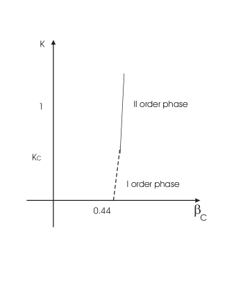
Figure 6: The diagram shows different phases of the system (2.5) as a function of the intersection coupling constant k. The partition function (2.6) is a function of temperature $\beta$ and of the coupling constant k. At $k=0$ the system (2.5), (2.6) reduces to (3.9), (4.18) and (4.22) with transfer matrix (4.23) and demonstrates, a strong first order phase transition. This is the ”supersymmetric” system defined in the sections 3 and 4. As the intersection coupling constant k increases, the first order phase transition is weakening, and at $k_{c}\approx 0.5$ the system undergoes a second order phase transition at $\beta_{c}\approx 0.44$ and has the critical indices ($\nu\approx 0.34$) which are different from those of the 3D Ising model ($\nu\approx 0.64$). These systems belong to different classes of universality. A similar behaviour demonstrates the system (2) in four dimensions. The critical behaviour and the phase structure of the gonihedric spin systems essentially depend on the intersection coupling constant k.

5 Monte-Carlo Simulation of Gonihedric Systems in Various Dimensions

The phase structure of the spin systems can be studied by using Monte-Carlo simulations [59, 60, 61]. The random surfaces with area action in four dimensions are defined through the one-plaquette self-dual gauge invariant action[23]. The simulations indicate that the phase transition is of the first order [24]. The four-dimensional Ising model exhibits critical behaviour with infinite correlation length and is supposed to be equivalent to a Higgs-like theory in the continuum limit [25, 26, 27, 28].

The simulations of the gonihedric system (2.5) in three dimensions demonstrate that it exhibits a second order phase transition [36, 37, 38, 42] (see Fig. 6). In four dimensions the system (2) also undergoes a second order phase transition[39, 40], suggesting that in the continuum limit there exists a string theory in four dimensions. A further study of the critical properties of the proposed models can be rewarding, specifically the scaling behaviour of the intersection lengths $<n_{4}>$ and $<n_{6}>$ [39, 40]. These are the disorder parameters of the system ( they vanish in the low-temperature phase and are non-zero at high-temperature phase ) defined as the derivative of the partition function (2.6) with respect to the coupling $k$. They represent the average length $\mu_{D}$ of the self-intersection edges (see Fig. 7)

$$\mu_{3}=-{1\over\beta}{\partial\ln Z\over\partial k}=4<n_{4}>,~{}~{}~{}\mu_{4}=-{1\over\beta}{\partial\ln Z\over\partial k}=<4\bar{n}_{4}+6\bar{\bar{n}}_{4}+12n_{6}>.$$ (5.27)

The second derivative with respect to $k$ defines the intersection susceptibility. These order parameters are analogous to the magnetisation in the case of Ising model and to the density in the case of liquid-gas transitions.

The other interesting property of the system is that the relaxation to the equilibrium state is very slow, like in spin glasses [20, 39, 41, 42, 43, 44, 45, 46, 51, 54, 52, 55, 56, 57, 58]. The reason is rooted in high symmetry of the system (3.9), its energy states are exponentially degenerated [17, 18, 19].

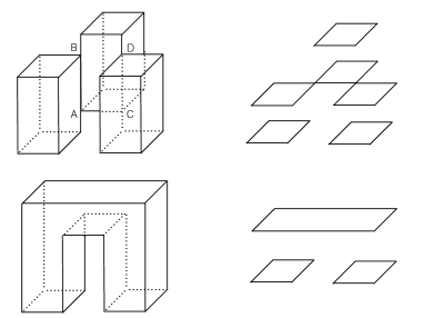
Figure 7: The diagrams on the left show the main topological types of surfaces with and without self-intersections. On the edges AB and CD take place the intersections of four plaquettes. The figures on the right show the horizontal ”time” slices of the surfaces. These time slices demonstrate that two initial strings propagate in the vertical direction, then interact and merge into the final string. The interaction ”time” is proportional to the length of the edges AB and CD. The intensity of string interactions is described by the intersection coupling constant k. In the limit $k\rightarrow\infty$ surfaces are self-avoiding.

6 Random Manifolds with Gonihedric Energy

Similar construction can be extended to the random manifolds of high dimension, that is, for three-, four- and higher-dimensional manifolds, sometimes called p-branes (p=2,3,..). We defined the corresponding energy functionals and transfer matrices, as well as equivalent spin systems[47, 48, 49]. This allows to simulate random manifolds of higher dimensionality on hypercubic lattices.

7 Memory Devices Based on Gonihedric Systems

The gonihedric spin systems are the systems of very high symmetry, their states are exponentially degenerate. The discovery and the understanding of these symmetry in [19, 20] was essential ingredient in the construction of the dual systems. The rate of degeneracy of the vacuum state depends on the self-intersection coupling constant $k$ [19, 20].

If $k\neq 0$, one can flip spins on any set of parallel planes and the degeneracy of the vacuum state is equal to $3\cdot 2^{N}$ for the lattice of the size $N^{3}$. The system with the self-intersection coupling constant $k=0$ is even more symmetric, one can flip spins $\sigma\rightarrow-\sigma$ on any set of planes orthogonal to the axis $x,y,z$ and is equal to $2^{3N}$ [19, 20].

These vacuum states, are separated by the potential barriers, therefore one can suggest to use such systems as storages of the binary information [50, 35]. Because there is no interface energy proportional to the area in these systems one can store one bit of information in a very small region of the gonihedric ”crystal”. It is an interesting and challenging problem to construct an artificial material which will have a corresponding structure.

References

- [1] Y. Nambu, ”Duality and Hydrodynamics” Lectures in Copenhagen Symposium (1970)
- [2] T. Goto, Relativistic quantum mechanics of one-dimensional mechanical continuum and subsidiary condition of dual resonance model, Prog. Theor. Phys. 46 (1971) 1560.
- [3] J. Ambjorn, B. Durhuus and J. Frohlich, Diseases of Triangulated Random Surface Models, and Possible Cures, Nucl. Phys. B 257 (1985) 433.
- [4] A. M. Polyakov, Fine Structure of Strings, Nucl. Phys. B 268 (1986) 406.
- [5] R. Ambartsumian, G.Sukiasian, G. Savvidy and K.Savvidy, Alternative model of random surfaces, Phys.Lett. B275 (1992) 99-102
- [6] G. Savvidy and K. Savvidy, Gonihedric string and asymptotic freedom, Mod.Phys.Lett. A8 (1993) 2963-2972
- [7] G. Savvidy and K. Savvidy, String fine tuning, Int.J.Mod.Phys. A8 (1993) 3993-4012
- [8] G. Savvidy and R. Manvelyan, Weyl invariant gonihedric strings, Phys. Lett. B 533 (2002) 138
- [9] G. Savvidy, Conformal invariant tensionless strings, Phys. Lett. B 552 (2003) 72.
- [10] G. Savvidy, Tensionless strings: Physical Fock space and higher spin fields, Int. J. Mod. Phys. A 19 (2004) 3171
- [11] G. Savvidy, Tensionless strings, correspondence with SO(D,D) sigma model, Phys. Lett. B 615 (2005) 285
- [12] J. Mourad, Continuous spin particles from a tensionless string theory, AIP Conf. Proc. 861 (2006) 436; hep-th/0504118.
- [13] G. Savvidy and R. Schneider, A lower estimate for the modified Steiner functional, Commun.Math.Phys. 161 (1994) 283-288
- [14] B. Durhuus and T. Jonsson, On subdivision invariant actions for random surfaces, Phys. Lett. B 297 (1992) 271
- [15] G. Koutsoumbas, G.Savvidy and K. Savvidy, Curvature representation of the gonihedric action, Europhys.Lett. 36 (1996) 331-336
- [16] G.Savvidy and F.Wegner, Geometrical string and spin systems, Nucl.Phys. B413 (1994) 605-613
- [17] G. Savvidy and K. Savvidy, Self-avoiding gonihedric string and spin systems, Phys.Lett. B324 (1994) 72-77
- [18] G. Savvidy and K. Savvidy, Interaction hierarchy, Phys.Lett. B337 (1994) 333-339
- [19] G.Savvidy , K. Savvidy and P. Savvidy Dual statistical systems and geometrical string, Phys.Lett. A (1994) 333-339
- [20] G. Savvidy, K. Savvidy and F. Wegner, Geometrical string and dual spin systems, Nucl.Phys. B443 (1995) 565-580
- [21] R.Pietig R and F. Wegner Phase transition in lattice surface systems with gonihedric action, Nucl.Phys.B466 (1996) 513
- [22] R.Pietig R and F. Wegner Low temperature expansion of the gonihedric Ising model, Nucl.Phys.B 525(1998) 549
- [23] F. J. Wegner, Duality in Generalized Ising Models and Phase Transitions Without Local Order Parameters, J. Math. Phys. 12 (1971) 2259.
- [24] M. Creutz, L. Jacobs and C. Rebbi, Experiments with a Gauge Invariant Ising System, Phys. Rev. Lett. 42 (1979) 1390.
- [25] K. G. Wilson, Critical Phenomena in 3.99 Dimensions, Physica 73 (1974) 119.
- [26] K. G. Wilson and J. B. Kogut, The Renormalization group and the epsilon expansion, Phys. Rept. 12 (1974) 75.
- [27] J. L. Cardy, Conformal Invariance and Statistical Mechanics, 169-246 ( Fields, Strings and Critical Phenomena: proceedings,1988. Les Houches, France. Edited by E. Brezin and J. Zinn-Justin. Amsterdam, North-Holland, 1990.)
- [28] M. Aizenman, Geometric Analysis of phi**4 Fields and Ising Models,I,II. Commun. Math. Phys. 86 (1982) 1.
- [29] T. Jonsson and G.Savvidy, Loop transfer matrix and gonihedric loop diffusion, Phys.Lett. B449 (1999) 253-259
- [30] T. Jonsson and G.Savvidy, The Spectrum of a transfer matrix for loops, Nucl.Phys. B575 (2000) 661-672
- [31] G. Savvidy, Loop transfer matrix and loop quantum mechanics, JHEP 0009 (2000) 044
- [32] M. Suzuki, Solution and Critical Behavior of Some ”Three-Dimensional” Ising Models with a Four-Spin Interaction, Phys. Rev. Lett. 28 (1972) 507
- [33] Y.Hashizume and M. Suzuki, New random ordered phase in isotropic models with many-body interactions, Int. J. Mod. Phys. AB25 (2011) 73
- [34] Y.Hashizume and M. Suzuki, Controlled randomness and frustration of the many-body interactions, Int. J. Mod. Phys. AB 25 (2012) 3529-3538.
- [35] C. Castelnovo, C. Chamon and D. Sherrington, Quantum mechanical and information theoretic view on classical glass transitions, Phys. Rev.B 81 (2010) 184303 .
- [36] G. Daskalakis and G. Savvidy, The Spectrum of the loop transfer matrix on finite lattice, Mod.Phys.Lett. A16 (2001) 1069-1078
- [37] G.Bathas, E.Floratos, G.Savvidy and K.Savvidy, Two and Three-Dimensional Spin Systems with Gonihedric Action, Mod.Phys.Lett. A 10 (1995) 2695-2701
- [38] G. Koutsoumbas and G. Savvidy, Three-dimensional gonihedric spin system, Mod.Phys.Lett. A17 (2002) 751
- [39] G. Koutsoumbas, G.Savvidy and K.Savvidy, Phase structure of four-dimensional gonihedric spin system, Phys.Lett. B410 (1997) 241-249
- [40] J. Ambjorn, G. Koutsoumbas and G. K. Savvidy, Four-dimensional gonihedric gauge spin system, Europhys. Lett. 46 (1999) 319
- [41] D. Johnston Gonihedric (and Fuki-Nuke) order J. Phys. A: Math. Theor.45 (2012) 405001
- [42] M.Baig M, D.Espriu, D. Johnston and R.Malmini, String tension in gonihedric 3-D Ising models, J.Phys.A:Math.Gen. 30 (1997) 405
- [43] A.Lipowski and D. Johnston, Glassy transition and metastability in four spin Ising model, J. Phys. A: Math. Gen. 33 ( 2000) 4451
- [44] A.Lipowski, D.Johnston and D.Espriu, Slow dynamics of Ising models with energy barriers, Phys Rev. E 62 (2000) 3404
- [45] M.Swift M, H.Bokil, R.Travasso and A. Bray, Glassy behavior in a ferromagnetic p-spin model, Phys. Rev. B 62 (2000) 11494
- [46] S. Davatolhagh, D.Dariush and L.Separdar Nature of the glassy transition in simulations of the ferromagnetic plaquette Ising model, Phys Rev. E 81 (2010 ) 031501
- [47] G. Savvidi and K. Savvidy Interaction hierarchy: String and quantum gravity, Mod.Phys.Lett. A11 (1996) 1379-1396
- [48] J. Ambjorn, G. Savvidy and K. Savvidy Alternative actions for quantum gravity and the intrinsic rigidity of the space-time, Nucl.Phys. B486 (1997) 390-412
- [49] G. Savvidy Quantum gravity with linear action. Intrinsic rigidity of space-time, Nucl.Phys.Proc.Suppl. 57 (1997) 104-114
- [50] G. Savvidy, The System with exponentially degenerate vacuum state, e-Print:cond-mat/ 0003220
- [51] F. Antenucci, M. I. Berganza and L. Leuzzi, Statistical physics of nonlinear wave interaction, arXiv:1412.8610 [cond-mat.stat-mech].
- [52] M. Mueller, D. A. Johnston and W. Janke, Exact solutions to plaquette Ising models with free and periodic boundaries, Nucl. Phys. B 914 (2017) 388. doi:10.1016/j.nuclphysb.2016.11.005
- [53] W. Janke, M. Mueller and D. A. Johnston, Finite-size scaling and latent heat at the gonihedric first-order phase transition, J. Phys. Conf. Ser. 640 (2015) 1, 012002. doi:10.1088/1742-6596/640/1/012002
- [54] D. A. Johnston, M. Mueller and W. Janke, Macroscopic degeneracy and order in the 3D plaquette Ising model, Mod. Phys. Lett. B 29 (2015) 20, 1550109. doi:10.1142/S0217984915501092
- [55] M. Mueller, W. Janke and D. A. Johnston, Planar ordering in the plaquette-only gonihedric Ising model, Nucl. Phys. B 894 (2015) 1 doi:10.1016/j.nuclphysb.2015.02.020 [arXiv:1412.4426 [cond-mat.stat-mech]].
- [56] M. Mueller, W. Janke and D. A. Johnston, Transmuted Finite-size Scaling at First-order Phase Transitions, Phys. Procedia 57 (2014) 68 doi:10.1016/j.phpro.2014.08.133 [arXiv:1410.7928 [cond-mat.stat-mech]].
- [57] M. Mueller, D. A. Johnston and W. Janke, Multicanonical analysis of the plaquette-only gonihedric Ising model and its dual, Nucl. Phys. B 888 (2014) 214 doi:10.1016/j.nuclphysb.2014.09.009 [arXiv:1407.7252 [cond-mat.stat-mech]].
- [58] M. Mueller, W. Janke and D. A. Johnston, Nonstandard Finite-Size Scaling at First-Order Phase Transitions, Phys. Rev. Lett. 112 (2014) 200601 doi:10.1103/PhysRevLett.112.200601 [arXiv:1312.5984 [cond-mat.stat-mech]].
- [59] G. Savvidy and N. Ter-Arutyunyan-Savvidy On the Monte Carlo simulation of physical systems, J.Comput.Phys. 97 (1991) 566
- [60] K. Savvidy The MIXMAX random number generator, arXiv: 1403.5355 (2014) 1
- [61] K. Savvidy and G. Savvidy, Spectrum and Entropy of C-systems. MIXMAX random number generator, Chaos Solitons Fractals 91 (2016) 33 doi:10.1016/j.chaos.2016.05.003 [arXiv:1510.06274 [math.DS]].