Glassy dynamics of athermal self-propelled particles: Computer simulations and a nonequilibrium microscopic theory

Abstract

We combine computer simulations and analytical theory to investigate the glassy dynamics in dense assemblies of athermal particles evolving under the sole influence of self-propulsion. Our simulations reveal that when the persistence time of the self-propulsion is increased, the local structure becomes more pronounced whereas the long-time dynamics first accelerates and then slows down. We explain these surprising findings by constructing a nonequilibrium microscopic theory which yields nontrivial predictions for the glassy dynamics. These predictions are in qualitative agreement with the simulations and reveal the importance of steady state correlations of the local velocities to the nonequilibrium dynamics of dense self-propelled particles.

I Introduction

The application of statistical mechanical methods to the dynamics of individual motile objects started shortly Furth after Einstein’s work on Brownian motion Einstein . Recently, the collective behavior of systems consisting of interacting self-propelled particles attracted interest Ramaswamyrev ; Marchettirev . An important motivation for studying ‘active’ systems is to understand spectacular dynamics observed in assemblies of living systems, such as coherent motion Bialek ; Dombrowski . A more fundamental motivation stems from the nonequilibrium nature of active systems that are driven by internal, non-thermal self-propulsion forces, which represents a difficult challenge for statistical physics. The behavior of such systems may defy our equilibrium-based physical intuition, as demonstrated by large-scale collective motion in persistent hard disk systems Deseigne , and the emergence of dynamic clustering Theurkauff ; Buttinoni , phase separation Buttinoni ; Redner ; Cates , and nonequilibrium equation of state Ginot ; Takatori ; Solon in repulsive self-propelled particles.

Active particles may also exhibit behavior similar to that found in equilibrium systems, such as crystallization Bialke1 . This behavior suggests that, like thermal systems BerthierBiroli , dense active systems could possibly be supercooled and exhibit glassy dynamics; as recently argued theoretically on the basis of a simple driven glassy model BerthierKurchan . This study was followed by numerical investigations of active particles with hard-core Ni ; Berthier or continuous Gompper ; Dasgupta interactions. Active glassy dynamics was observed, but when compared with thermal systems, the onset of glassy behavior was always pushed towards higher densities and lower temperatures. When self-propulsion is progressively added to an otherwise thermal system, it was noted that the local structure becomes less pronounced Ni ; Dasgupta . Such change in local structure suggests both a simple physical explanation for the shift of the onset of glassy behavior, and that a straightforward extension of mode-coupling theory Goetzebook can describe this shift BerthierKurchan ; Farage .

Here we present a simulational and theoretical study of the structure and glassy dynamics of a more complex system in which self-propulsion is the only source of motion. We study self-propelled particles interacting with a continuous potential (differently from Ni ; Berthier ) and without thermal Brownian motion (differently from Ni ; Bialke1 ; Gompper ). Thus, our model is ‘athermal’ Fily ; Berthier , and the degree of nonequilibrium is quantified by the persistence time $\tau_{p}$ of the self-propulsion. As $\tau_{p}$ increases at a constant effective temperature, we find that the structure of the system becomes more pronounced, whereas the dynamics initially speeds up and then slows down, showing that in our model the shift of the glassy dynamics with self-propulsion is not simply the direct consequence of the changing microstructure Farage ; Dasgupta .

To elucidate these findings we develop a microscopic theory that accounts for the nonequilibrium nature of athermal self-propelled systems. We are aware of no other approach where many-body interactions are taken into account at the microscopic level. The theory is constructed from the steady state structure factor and the steady state correlations of the velocities. The latter correlations are non-trivial only for self-propelled systems with a finite persistence time, and are central to explain the opposite, and seemingly contradictory, evolution of the structure and dynamics in dense active materials.

II Model active system

We study a system of interacting self-propelled particles in a viscous medium. We model self-propulsion as an internal driving force evolving according to the Ornstein-Uhlenbeck VanKampen process:

$$\dot{\mathbf{r}}_{i} = \xi_{0}^{-1}\left[\mathbf{F}_{i}+\mathbf{f}_{i}\right],$$ (1)

$$\dot{\mathbf{f}}_{i} = -\tau_{p}^{-1}\mathbf{f}_{i}+\bm{\eta}_{i}.$$ (2)

In Eq. (1), $\mathbf{r}_{i}$ is the position of particle $i$, $\xi_{0}$ the friction coefficient of an isolated particle, $\mathbf{F}_{i}$ is the force acting on particle $i$ originating from interactions, $\mathbf{F}_{i}=-\sum_{j\neq i}\bm{\nabla}_{i}V(r_{ij})$, and $\mathbf{f}_{i}$ is the self-propulsion acting on particle $i$. In Eq. (2), $\tau_{p}$ is the persistence time of the self-propulsion and $\bm{\eta}_{i}$ is an internal Gaussian noise with zero mean and variance $\left<\bm{\eta}_{i}(t)\bm{\eta}_{j}(t^{\prime})\right>_{\text{noise}}=2D_{f}\bm{I}\delta_{ij}\delta(t-t^{\prime})$, where $\left<...\right>_{\text{noise}}$ denotes averaging over the noise distribution, $D_{f}$ is the noise strength and $\bm{I}$ is the unit tensor. Without interactions, Eqs. (1-2) produce a persistent random walk with a self-diffusion coefficient $D_{0}=D_{f}\tau_{p}^{2}/\xi_{0}^{2}$, which defines the single-particle effective temperature: $T_{\text{eff}}=D_{0}\xi_{0}=D_{f}\tau_{p}^{2}/\xi_{0}$ toy . It is convenient to choose as three independent control parameters the number density $\rho$ (which is kept fixed), the effective temperature $T_{\text{eff}}$, and the persistence time $\tau_{p}$. The persistence time quantifies the degree of nonequilibrium; when $\tau_{p}\to 0$ our system becomes equivalent to a Brownian system at temperature $T=T_{\text{eff}}$. Including additional thermal noise would add a fourth control parameter to the model. Finally, we should mention that recently an approximate mapping has been derived FarageKB between our model and the standard active Brownian particles model tenHagen .

III Computer simulation study

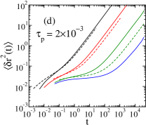
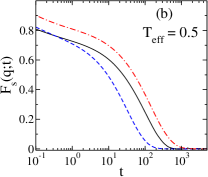
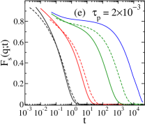
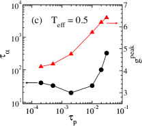
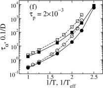
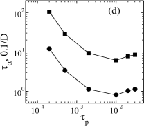
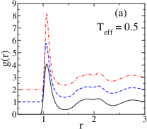
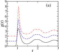
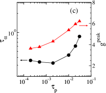
Figure 1: Evolution of the structure and dynamics with the persistence time $\tau_{p}$ at $T_{\text{eff}}=0.5$ (a-c) and comparison of dynamics in active systems with $\tau_{p}=2\times 10^{-3}$ and Brownian systems at $T=T_{\rm eff}=0.5$ (d-f). In (a,b) solid lines correspond to $\tau_{p}=0$ (equivalent to a thermal system at $T=0.5$), and the dashed, and dot-dashed lines correspond to $\tau_{p}=2\times 10^{-3}$, and $2\times 10^{-2}$, respectively. In (a) we show the pair distribution function $g(r)$; the curves are shifted vertically for clarity. In (b) we show the self-intermediate scattering function $F_{s}(q;t)=\langle e^{i\mathbf{q}\cdot(\mathbf{r}_{j}(t)-\mathbf{r}_{j}(0))}\rangle$ for $q=7.25$. In (c) we show the relaxation time, $\tau_{\alpha}$ (circles) and the peak value of $g(r)$ (triangles). The relaxation time is defined as $F_{s}(q;\tau_{\alpha})=e^{-1}$. In (d,e) solid lines correspond to active systems at $T_{\text{eff}}=1$, 0.6, 0.45 and 0.4, and dashed lines correspond to equilibrium systems at $T=1$, 0.6 and 0.45 (from left to right). In (d) we show mean-square displacement $\left<\delta r^{2}(t)\right>=\left<(\mathbf{r}_{j}(t)-\mathbf{r}_{j}(0))^{2}\right>$ and in (e) we show $F_{s}(q;t)$. In (f) circles represent $\tau_{\alpha}$, squares represent the inverse self-diffusion coefficient, $0.1/D$ of active (closed symbols) and thermal (open symbols) systems.

To compare the glassy behavior of the self-propelled system with that of a well-studied thermal system, we simulated the Kob-Andersen (KA) binary mixture Kob1994 . All quantities presented pertain to the large particles, which comprise 80% of the mixture. The results are presented in reduced units units at the well-studied density $\rho=1.2$. In panels (a-c) of Fig. 1 we show the dependence of the structure and dynamics when moving away from equilibrium by increasing the persistence time of the self-propulsion at constant $T_{\text{eff}}=0.5$ commentT . At $T=0.5$ the thermal KA system exhibits glassy dynamics. In panels (a,c), we see that the pair correlation $g(r)$ of the active fluid becomes more structured at all length scales with increasing $\tau_{p}$. In equilibrium, such behavior is usually accompanied by slower dynamics. Surprisingly, panels (b,c) show that the nonequilibrium dynamics exhibits a non-monotonic dependence on $\tau_{p}$, which allows one to define an ‘optimal’ value for $\tau_{p}$. Describing the contrasting dependencies of structure and dynamics is a theoretical challenge since most microscopic glass theories predict the dynamics on the basis of the pair structure BerthierBiroli ; Gilles . A reentrant behavior of the dynamics in driven glassy dynamics is typically not observed BerthierKurchan ; Ni ; Berthier ; Gompper ; Dasgupta . In panels (e,f) we show that, if the persistence time is chosen at its optimal value, the dependence of the dynamics of the self-propelled system on $T_{\rm eff}$ is weaker than that of the thermal Brownian system on $T$. In particular, we can study the self-propelled system at $T_{\text{eff}}=0.4$, whereas it is challenging to simulate the thermal system below $T\approx 0.43$. The opposite is true for longer persistence times, where the dependence of the dynamics of the self-propelled system on $T_{\rm eff}$ becomes significantly more pronounced than that of the thermal Brownian system.

IV Theory

We now outline a microscopic theory for the time dependence of the collective intermediate scattering function, $F(q;t)$, of our model active system commentFs ,

$$F(q;t)=N^{-1}\left<n(\mathbf{q})e^{\Omega t}n(-\mathbf{q})\right>.$$ (3)

In Eq. (3), $N$ is the number of particles, $n(\mathbf{q})=\sum_{j}e^{-i\mathbf{q}\cdot\mathbf{r}_{j}}$ is the Fourier transform of the microscopic density, and $\Omega$ is the $N$-particle evolution operator that can be derived from the equations of motion (1-2):

$$\Omega=-\xi_{0}^{-1}\sum_{i}\bm{\nabla}_{i}\cdot\left(\mathbf{f}_{i}+\mathbf{F}_{i}\right)+\sum_{i}\frac{\partial}{\partial\mathbf{f}_{i}}\cdot\left(\tau_{p}^{-1}\mathbf{f}_{i}+D_{f}\frac{\partial}{\partial\mathbf{f}_{i}}\right).$$ (4)

Finally $\left<\dots\right>$ in (3) denotes an average over a steady state distribution of positions and self-propulsions; the steady state distribution stands to the right of the quantity being averaged, and all operators act on it too. In our approach, we first integrate out the self-propulsions and then we use the projection operator method, and a mode-coupling-like approximation to derive an approximate equation of motion for $F(q;t)$.

To begin, we briefly discuss the case of non-interacting particles. In this case one could start from the Laplace transform of Eq. (3) with the evolution operator similar to (4) but without interactions. In the simplest approximation, after integration over self-propulsions one gets

$$F(q;z)=N^{-1}\left<n(\mathbf{q})\left(z-\Omega^{\text{eff}}_{\text{free}}(z)\right)^{-1}n(-\mathbf{q})\right>_{\bf r},$$ (5)

where $\Omega^{\text{eff}}_{\text{free}}(z)=\xi_{0}^{-2}\sum_{i}\bm{\nabla}_{i}\left(z+\tau_{p}^{-1}\right)^{-1}D_{f}\tau_{p}\cdot\bm{\nabla}_{i}$ and $\left<...\right>_{\bf r}$ denotes the steady state average over particles positions. According to $\Omega^{\text{eff}}_{\text{free}}(z)$, particle motion is ballistic at short times and diffusive at long times, with the long-time self-diffusion coefficient $D_{0}$ discussed above.

For interacting particles, the integration over self-propulsions is more complicated due to non-trivial correlations between positions and self-propulsions (already present for a single self-propelled particle in an external potential toy ). As we show in Appendix A, the final result is a formula analogous to Eq. (5) but with the following evolution operator,

$$\Omega^{\text{eff}}(z)=\xi_{0}^{-2}\sum_{i,j}\bm{\nabla}_{i}\cdot\left(z+\tau_{p}^{-1}\right)^{-1}$$ (6)

$$\left(\left<\mathbf{f}_{i}\mathbf{f}_{j}\right>_{\text{lss}}-\left<\mathbf{f}_{i}\right>_{\text{lss}}\left<\mathbf{f}_{j}\right>_{\text{lss}}\right)\cdot\left[-\mathbf{F}_{j}^{\text{\text{eff}}}+\bm{\nabla}_{j}\right].$$

Here, $\left<...\right>_{\text{lss}}$ is an average over the conditional steady state distribution of self-propulsions, $P_{N}^{\text{ss}}(\mathbf{r}_{1},\mathbf{f}_{1},...,\mathbf{r}_{N},\mathbf{f}_{N})/P_{N}^{\text{ss}}(\mathbf{r}_{1},...,\mathbf{r}_{N})$, where the superscript ‘ss’ stands for ‘steady state’. Furthermore, $\mathbf{F}_{j}^{\text{\text{eff}}}=\bm{\nabla}_{j}\ln P_{N}^{\text{ss}}(\mathbf{r}_{1},...,\mathbf{r}_{N})$ is the effective force acting on particle $j$ in the steady state. The most important physical assumption used in the derivation of Eq. (6) is the absence of systematic currents in the steady state, see Appendix A. We expect the persistence time to be renormalized by the interactions; the presence of the bare persistence time in Eq. (6) represents an approximation.

We now use the projection operator method and arrive at the following memory function equation,

$$\partial^{2}_{t}F(q;t)+\tau_{p}^{-1}\partial_{t}F(q;t)=$$

$$-\frac{\omega_{\parallel}(q)q^{2}}{S(q)}F(q;t)-\int_{0}^{t}dt^{\prime}M^{\text{irr}}(q;t-t^{\prime})\partial_{t^{\prime}}F(q;t^{\prime}).$$

Here, $S(q)=\left<n(\mathbf{q})n(-\mathbf{q})\right>$ is the steady state structure factor, $\omega_{\parallel}(q)=\left(N\xi_{0}^{2}\right)^{-1}\left<\left|\hat{\mathbf{q}}\cdot\sum_{i}\left(\mathbf{f}_{i}+\mathbf{F}_{i}\right)e^{-i\mathbf{q}\cdot\mathbf{r}_{i}}\right|^{2}\right>$ quantifies correlations of the velocities of individual particles commentv , and $M^{\text{irr}}(q;t)$ is the irreducible memory function. The presence of the second time derivative in Eq. (IV) reflects the ballistic nature of the short-time motion. A comparison of Eq. (IV) with the analogous equation for an underdamped thermal system suggests to interpret $\tau_{p}\omega_{\parallel}(q)/S(q)$ as a short-time collective diffusion coefficient. Since this coefficient involves $\omega_{\parallel}(q)$, even in the absence of the memory function we need two static correlation functions to predict the dynamics, $S(q)$ and $\omega_{\parallel}(q)$. Whereas the emergence of velocity correlations can be generically expected far from equilibrium, the specific role they play for self-propelled systems is non-trivial and was not identified before.

The main approximation of our theory is a factorization approximation for the memory function to close the dynamical equations. This is analogous to the mode-coupling approximation Goetzebook . As we show in Appendix B, using the factorization approximation and an approximation for the steady state vertex function, we arrive at the following expression for the memory function,

$$M^{\mathrm{irr}}(q;t) = \frac{\rho\omega_{\parallel}(q)}{2}\int\frac{d\mathbf{q}_{1}d\mathbf{q}_{2}}{(2\pi)^{3}}\delta(\mathbf{q}-\mathbf{q}_{1}-\mathbf{q}_{2})$$

$$\times\left(\hat{\mathbf{q}}\cdot\left[\mathbf{q}_{1}\mathcal{C}(q_{1})+\mathbf{q}_{2}\mathcal{C}(q_{2})\right]\right)^{2}F(q_{1};t)F(q_{2};t).$$

Equation (IV) has a structure similar to the memory function of the mode-coupling theory, but it involves a new function $\mathcal{C}(q)$ (which replaces the direct correlation function $c(q)$ in the mode-coupling $M^{\text{irr}}(q;t)$),

$$\displaystyle\rho\mathcal{C}(q)=1-\frac{\omega_{\parallel}(q)}{\omega_{\parallel}(\infty)S(q)},$$ (9)

where $\omega_{\parallel}(\infty)=\left(3N\xi_{0}^{2}\right)^{-1}\left<\sum_{i}\left(\mathbf{f}_{i}+\mathbf{F}_{i}\right)^{2}\right>$. Equations (IV-9) are closed and can be solved if static steady state functions $S(q)$ and $\omega_{\parallel}(q)$ are available. To test the theory quantitatively, we used the static information obtained directly from simulations. Using the KA system would require formulating and solving our theory for a binary mixture. Instead, we performed additional simulations of a one-component Lennard-Jones (LJ) system of self-propelled particles commentLJ . We measured $S(q)$ and $\omega_{\parallel}(q)$ and used them to solve Eqs. (IV-9) numerically to compare the dynamics predicted by the theory with the numerical results. We focus on the observed non-monotonic evolution of the dynamics with the persistence time because it represents a demanding test of the theory.

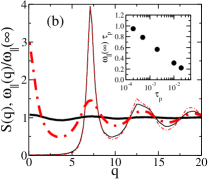
Figure 2: Structure (a,b) and dynamics (c) obtained from simulations, and predicted by the theory (d) for various $\tau_{p}$ at $T_{\text{eff}}=0.9$ in the one-component LJ system. (a) Pair distribution function $g(r)$; the curves are shifted vertically for clarity; $\tau_{p}=0,2\times 10^{-3}$, and $2\times 10^{-2}$ (bottom to top). In (b) thick lines represent $\omega_{\parallel}(q)/\omega_{\parallel}(\infty)$ and thin lines represent $S(k)$ at $\tau_{p}=2\times 10^{-4}$ (solid) and $2\times 10^{-2}$ (dashed). The inset in (b) shows the persistence time dependence of $\omega_{\parallel}(\infty)\tau_{p}$. In (c) we show $\tau_{\alpha}$ (circles, left axis) and the peak value of $g(r)$ (triangles, right axis), obtained from simulations. In (d) we show $\tau_{\alpha}$ (circles) and the inverse self-diffusion coefficient, $0.1/D$ (squares) predicted by the theory.

In Fig. 2(a-c) we show the dependence of $g(r)$, $S(q)$ and $\omega_{\parallel}(q)/\omega_{\parallel}(\infty)$ of the self-propelled LJ system on the persistence time $\tau_{p}$ at constant $T_{\text{eff}}=0.9$ (this is the lowest $T_{\text{eff}}$ at which we were able to simulate our one-component system without observing spontaneous ordering). Again, the structure becomes progressively more pronounced as $\tau_{p}$ increases. Concurrently, correlations of particle velocities also develop, as revealed by $\omega_{\parallel}(q)/\omega_{\parallel}(\infty)$. Finally, the quantity $\omega_{\parallel}(\infty)\tau_{p}$, which is a measure of local mobility in the interacting self-propelled system, decreases.

Because it incorporates these different trends, our theory is able to account for the non-monotonic dependence of the dynamics on the persistence time. In particular, with increasing $\tau_{p}$ both $S(q)$ and $\omega_{\parallel}(q)$ grow for $q$ around $2\pi/\sigma$ and as a result $\mathcal{C}(q)$ gets smaller than $c(q)$, which is the likely source of the speed-up in the dynamics. At larger $\tau_{p}$ decreasing $\omega_{\parallel}(\infty)\tau_{p}$ and increasingly more pronounced local structure seem to prevail upon the increase in velocity correlations resulting in the slowing down in the dynamics. In panels (c,d), we show the dynamics predicted by the theory and obtained from simulations, respectively. Clearly, our theory qualitatively predicts the non-monotonic dependence of the dynamics on the persistence time, suggesting that including non-equilibrium velocity correlations $\omega_{\parallel}(q)$ in the theory is of major importance. Mode-coupling theories overestimate the slowing down of the dynamics Goetzebook , and this explains why our theory predicts a more pronounced non-monotonic effect than in the simulations. Describing quantitatively glassy dynamics at thermal equilibrium is a notoriously difficult and open challenge BerthierBiroli . Therefore, quantitative agreement should not be expected in the far from equilibrium context of self-propelled particles.

Various kinds of generalizations of mode-coupling theory for driven glassy fluids have been proposed BerthierKurchan ; Farage ; Sperl ; BBK ; Reichman ; Fuchs . In particular, Ref. Farage developed a theory for active Brownian particles, where self-propulsion is added to a thermal Brownian system, but this work differs from our approach on important aspects. First, correlations between positions and self-propulsions were neglected in Farage . Technically, this amounts to replacing the local steady-state average in Eq. (6) by the average over the distribution of self-propulsions. As a result, $\left(\left<\mathbf{f}_{i}\mathbf{f}_{j}\right>_{\text{lss}}-\left<\mathbf{f}_{i}\right>_{\text{lss}}\left<\mathbf{f}_{j}\right>_{\text{lss}}\right)$ gets replaced by $D_{f}\tau_{p}\delta_{ij}\bm{I}$, and the steady state correlation function $\omega_{\parallel}(q)$, which we have shown to play a central role, does not appear. Second, in our derivation we use projection operators defined in terms of the steady state distribution, whereas Ref. Farage uses the equilibrium distribution. As a result, the memory function derived in Ref. Farage is the same as in the equilibrium mode-coupling theory while ours is different. Because we consider an intrinsically nonequilibrium system, there is no equilibrium distribution that we could use. Physically, the steady state distribution seems more natural since we are describing fluctuations in the steady state. An obvious disadvantage of our choice is that we have to obtain the steady state correlation functions, $S(q)$ and $\omega_{\parallel}(q)$, from simulations.

V Summary

Using computer simulations and tools from liquid state theory we developed and analyzed an athermal system of interacting self-propelled particles. We showed that the microscopic structure and long-time dynamics evolve nontrivially with the degree of nonequilibrium, which challenges equilibrium theories for dense fluids. We presented a theory for the collective dynamics of an active many-body system that can qualitatively capture these phenomena. In particular, the speed up of the dynamics of the active fluid was linked to emerging steady state correlations of the velocities, an object with no relevant equilibrium counterpart. In future work, we will numerically characterize the approach to the glass transition in more detail for such nonequilibrium conditions. On the theory side, we will analyze the nature of the ‘nonequilibrium glass transition’ BerthierKurchan predicted by our theory. We shall also compare the dynamics predicted by the theory with that obtained from simulations at larger degrees of supercooling, and the relation between the ergodicity breaking temperature predicted by our theory with the transition temperature obtained from simulations. To perform detailed quantitative comparisons, we will need to generalize the present results to binary mixtures. More generally, our work paves the way for developing a general, microscopic understanding of the glassy dynamics of active materials when different interparticle interactions, self-propulsion mechanisms and possibly thermal noise are at play.

Appendix A Derivation of effective evolution operator $\Omega^{\text{eff}}(z)$

In Appendix A we present an outline of a derivation of the effective $N$-particle evolution operator $\Omega^{\text{eff}}(z)$, Eq. (6). There are three main assumptions used in this derivation. First, we assume that systematic currents vanish in the steady state of our system. Second, we assume a separation of timescales for the structural relaxation and the relaxation of the self-propulsions. Third, we approximate the dynamics in the space orthogonal to the local equilibrium distribution of self-propulsions by the free relaxation of the self-propulsions.

Equations of motion (1-2) are equivalent to the following evolution equation for the $N$-particle joint distribution of positions and self-propulsions,

$$\partial_{t}P_{N}(\mathbf{r}_{1},\mathbf{f}_{1},...,\mathbf{r}_{N},\mathbf{f}_{N};t)=\Omega P_{N}(\mathbf{r}_{1},\mathbf{f}_{1},...,\mathbf{r}_{N},\mathbf{f}_{N};t)$$

where $\Omega$ is the $N$-particle evolution operator given by Eq. (4).

We assume that the evolution equation (A) has a steady state solution $P_{N}^{\text{ss}}(\mathbf{r}_{1},\mathbf{f}_{1},...,\mathbf{r}_{N},\mathbf{f}_{N})$, and thus

$$\Omega P_{N}^{\text{ss}}(\mathbf{r}_{1},\mathbf{f}_{1},...,\mathbf{r}_{N},\mathbf{f}_{N})=0.$$ (11)

In the main text and in the following we use brackets $\left<\dots\right>$ to denote averaging over the joint steady state distribution of positions and self-propulsions, $P_{N}^{\text{ss}}(\mathbf{r}_{1},\mathbf{f}_{1},...,\mathbf{r}_{N},\mathbf{f}_{N})$.

From the joint steady state distribution we can obtain a steady state distribution of positions, $P_{N}^{\text{ss}}(\mathbf{r}_{1},...,\mathbf{r}_{N})$,

$$P_{N}^{\text{ss}}(\mathbf{r}_{1},...,\mathbf{r}_{N})=\int d\mathbf{f}_{1}...d\mathbf{f}_{N}P_{N}^{\text{ss}}(\mathbf{r}_{1},\mathbf{f}_{1},...,\mathbf{r}_{N},\mathbf{f}_{N}).$$ (12)

In the main text and in the following we use brackets $\left<\dots\right>_{\mathbf{r}}$ to denote averaging over a steady state distribution of positions, $P_{N}^{\text{ss}}(\mathbf{r}_{1},...,\mathbf{r}_{N})$.

We assume that in the steady state there are no systematic currents. To make this statement more precise we first define the current density by integrating Eq. (A) over self-propulsions to get the following continuity equation,

$$\partial_{t}P_{N}(\mathbf{r}_{1},...,\mathbf{r}_{N};t)=-\sum_{i}\bm{\nabla}_{i}\cdot\mathbf{j}_{i}(\mathbf{r}_{1},...,\mathbf{r}_{N};t),$$ (13)

where $P_{N}(\mathbf{r}_{1},...,\mathbf{r}_{N};t)$ is the N-particle distribution of positions,

$$P_{N}(\mathbf{r}_{1},...,\mathbf{r}_{N};t)=\int d\mathbf{f}_{1}...d\mathbf{f}_{N}P_{N}(\mathbf{r}_{1},\mathbf{f}_{1},...,\mathbf{r}_{N},\mathbf{f}_{N};t),$$ (14)

and $\mathbf{j}_{i}(\mathbf{r}_{1},...,\mathbf{r}_{N};t)$ is the current density of particle $i$,

$$\mathbf{j}_{i}(\mathbf{r}_{1},...,\mathbf{r}_{N};t)=$$

$$\xi_{0}^{-1}\int d\mathbf{f}_{1}...d\mathbf{f}_{N}\left(\mathbf{F}_{i}+\mathbf{f}_{i}\right)P_{N}(\mathbf{r}_{1},\mathbf{f}_{1},...,\mathbf{r}_{N},\mathbf{f}_{N};t).$$

Our assumption of the absence of systematic currents in the steady state is implemented as follows,

$$\xi_{0}^{-1}\int d\mathbf{f}_{1}...d\mathbf{f}_{N}\left[\mathbf{F}_{i}+\mathbf{f}_{i}\right]P_{N}^{\text{ss}}(\mathbf{r}_{1},\mathbf{f}_{1},...,\mathbf{r}_{N},\mathbf{f}_{N})=0.$$ (16)

The above equality implies that the local steady state average of the self-propulsion is equal to the negative of the force, $\left<\mathbf{f}_{i}\right>_{\text{lss}}=-\mathbf{F}_{i}$, where the local steady state average is defined as

$$\left<\dots\right>_{\text{lss}}=$$

$$\frac{1}{P_{N}^{\text{ss}}(\mathbf{r}_{1},...,\mathbf{r}_{N})}\int d\mathbf{f}_{1}...d\mathbf{f}_{N}\dots P_{N}^{\text{ss}}(\mathbf{r}_{1},\mathbf{f}_{1},...,\mathbf{r}_{N},\mathbf{f}_{N}).$$

We assume that the self-propulsions relax faster than the positions of the particles. This assumption is applicable for strongly interacting systems where structural relaxation is slowing down, whereas the evolution of the self-propulsions stays, by definition, independent of intermolecular interactions. The separation of the timescales for the structural and self-propulsions relaxations allows us to derive an approximate equation of motion for the distribution of particle positions.

We define the projection operator on a local equilibrium-like distribution (i.e. on a distribution in which self-propulsions have a steady-state distribution for a given sample of positions),

$$\mathcal{P}_{\text{lss}}P_{N}(\mathbf{r}_{1},\mathbf{f}_{1},...,\mathbf{r}_{N},\mathbf{f}_{N};t)=$$ (18)

$$=\frac{P_{N}^{\text{ss}}(\mathbf{r}_{1},\mathbf{f}_{1},...,\mathbf{r}_{N},\mathbf{f}_{N})}{P_{N}^{\text{ss}}(\mathbf{r}_{1},...,\mathbf{r}_{N})}\int d\mathbf{f}_{1}...d\mathbf{f}_{N}P_{N}(\mathbf{r}_{1},\mathbf{f}_{1},...,\mathbf{r}_{N},\mathbf{f}_{N};t)$$

$$=\frac{P_{N}^{\text{ss}}(\mathbf{r}_{1},\mathbf{f}_{1},...,\mathbf{r}_{N},\mathbf{f}_{N})}{P_{N}^{\text{ss}}(\mathbf{r}_{1},...,\mathbf{r}_{N})}P_{N}(\mathbf{r}_{1},...,\mathbf{r}_{N};t).$$

Next, we define the orthogonal projection, $\mathcal{Q}_{\text{lss}}=\mathcal{I}-\mathcal{P}_{\text{lss}}$, and write down equations of motion for $\mathcal{P}_{\text{lss}}P_{N}(\mathbf{r}_{1},\mathbf{f}_{1},...,\mathbf{r}_{N},\mathbf{f}_{N};t)$ and $\mathcal{Q}_{\text{lss}}P_{N}(\mathbf{r}_{1},\mathbf{f}_{1},...,\mathbf{r}_{N},\mathbf{f}_{N};t)$,

$$\partial_{t}\mathcal{P}_{\text{lss}}P_{N}(\mathbf{r}_{1},\mathbf{f}_{1},...,\mathbf{r}_{N},\mathbf{f}_{N};t)=$$ (19)

$$\mathcal{P}_{\text{lss}}\Omega\mathcal{P}_{\text{lss}}P_{N}(\mathbf{r}_{1},\mathbf{f}_{1},...,\mathbf{r}_{N},\mathbf{f}_{N};t)$$

$$+\mathcal{P}_{\text{lss}}\Omega\mathcal{Q}_{\text{lss}}P_{N}(\mathbf{r}_{1},\mathbf{f}_{1},...,\mathbf{r}_{N},\mathbf{f}_{N};t),$$

$$\partial_{t}\mathcal{Q}_{\text{lss}}P_{N}(\mathbf{r}_{1},\mathbf{f}_{1},...,\mathbf{r}_{N},\mathbf{f}_{N};t)=$$ (20)

$$\mathcal{Q}_{\text{lss}}\Omega\mathcal{P}_{\text{lss}}P_{N}(\mathbf{r}_{1},\mathbf{f}_{1},...,\mathbf{r}_{N},\mathbf{f}_{N};t)$$

$$+\mathcal{Q}_{\text{lss}}\Omega\mathcal{Q}_{\text{lss}}P_{N}(\mathbf{r}_{1},\mathbf{f}_{1},...,\mathbf{r}_{N},\mathbf{f}_{N};t).$$

Since our final goal is to calculate the intermediate scattering function given by Eq. (3), we can assume that $\mathcal{Q}_{\text{lss}}P_{N}(\mathbf{r}_{1},\mathbf{f}_{1},...,\mathbf{r}_{N},\mathbf{f}_{N};t=0)=0$. Then we can solve Eqs. (19-20) for the Laplace transform, $\mathcal{LT}$, of $\partial_{t}\mathcal{P}_{\text{lss}}P_{N}(\mathbf{r}_{1},\mathbf{f}_{1},...,\mathbf{r}_{N},\mathbf{f}_{N};t)$, which is given by

$$\mathcal{LT}\left[\partial_{t}\mathcal{P}_{\text{lss}}P_{N}(\mathbf{r}_{1},\mathbf{f}_{1},...,\mathbf{r}_{N},\mathbf{f}_{N};t)\right](z)=\left[\mathcal{P}_{\text{lss}}\Omega\mathcal{P}_{\text{lss}}+\mathcal{P}_{\text{lss}}\Omega\mathcal{Q}_{\text{lss}}\frac{1}{z-\mathcal{Q}_{\text{lss}}\Omega\mathcal{Q}_{\text{lss}}}\mathcal{Q}_{\text{lss}}\Omega\mathcal{P}_{\text{lss}}\right]\mathcal{P}_{\text{lss}}P_{N}(\mathbf{r}_{1},\mathbf{f}_{1},...,\mathbf{r}_{N},\mathbf{f}_{N};z).$$

Using the assumption that systematic currents vanish in the steady state, Eq. (16), one can show that the first term inside the brackets on right-hand-side of Eq. (A) vanishes. Furthermore, one can show that

$$\mathcal{Q}_{\text{lss}}\Omega\mathcal{P}_{\text{lss}}P_{N}(z)=-\xi_{0}^{-1}\sum_{i}\left(\mathbf{f}_{i}-\left<\mathbf{f}_{i}\right>_{\text{lss}}\right)P_{N}^{\text{ss}}(\mathbf{r}_{1},\mathbf{f}_{1},...,\mathbf{r}_{N},\mathbf{f}_{N})\cdot\left[\bm{\nabla}_{i}\frac{P_{N}(\mathbf{r}_{1},...,\mathbf{r}_{N};z)}{P_{N}^{\text{ss}}(\mathbf{r}_{1},...,\mathbf{r}_{N})}\right]$$ (22)

and

$$\mathcal{P}_{\text{lss}}\Omega\mathcal{Q}_{\text{lss}}...=-\frac{P_{N}^{\text{ss}}(\mathbf{r}_{1},\mathbf{f}_{1},...,\mathbf{r}_{N},\mathbf{f}_{N})}{P_{N}^{\text{ss}}(\mathbf{r}_{1},...,\mathbf{r}_{N})}\xi_{0}^{-1}\sum_{i}\bm{\nabla}_{i}\cdot\int d\mathbf{f}_{1}...d\mathbf{f}_{N}\left(\mathbf{f}_{i}-\left<\mathbf{f}_{i}\right>_{\text{lss}}\right)...$$ (23)

We note that $\mathcal{Q}_{\text{lss}}\Omega\mathcal{Q}_{\text{lss}}$ describes evolution in the space orthogonal to the local steady state space. We assume that this evolution is entirely due to the free relaxation of the self-propulsions. Specifically, we assume that $\mathcal{Q}_{\text{lss}}\Omega\mathcal{Q}_{\text{lss}}$ can be approximated by $\sum_{i=1}^{N}\frac{\partial}{\partial\mathbf{f}_{i}}\left(\tau_{p}^{-1}\mathbf{f}_{i}+D_{f}\frac{\partial}{\partial\mathbf{f}_{i}}\right)$. We note that this approximation physically means that the relaxation rate of the self-propulsions is not renormalized by the interparticle interactions. Combining the last approximation with Eqs. (22-23) we get the following approximate equality

$$\mathcal{P}_{\text{lss}}\Omega\mathcal{Q}_{\text{lss}}\left(z-\mathcal{Q}_{\text{lss}}\Omega\mathcal{Q}_{\text{lss}}\right)^{-1}\mathcal{Q}_{\text{lss}}\Omega\mathcal{P}_{\text{lss}}P_{N}(\mathbf{r}_{1},\mathbf{f}_{1},...,\mathbf{r}_{N},\mathbf{f}_{N};z)\approx$$ (24)

$$\frac{P_{N}^{\text{ss}}(\mathbf{r}_{1},\mathbf{f}_{1},...,\mathbf{r}_{N},\mathbf{f}_{N})}{P_{N}^{\text{ss}}(\mathbf{r}_{1},...,\mathbf{r}_{N})}\xi_{0}^{-2}\sum_{i}\bm{\nabla}_{i}\cdot\int d\mathbf{f}_{1}...d\mathbf{f}_{N}\left(\mathbf{f}_{i}-\left<\mathbf{f}_{i}\right>_{\text{lss}}\right)$$

$$\times\left[z-\sum_{j=1}^{N}\frac{\partial}{\partial\mathbf{f}_{j}}\left(\tau_{p}^{-1}\mathbf{f}_{j}+D_{f}\frac{\partial}{\partial\mathbf{f}_{j}}\right)\right]^{-1}\sum_{l}\left(\mathbf{f}_{l}-\left<\mathbf{f}_{l}\right>_{\text{lss}}\right)P_{N}^{\text{ss}}(\mathbf{r}_{1},\mathbf{f}_{1},...,\mathbf{r}_{N},\mathbf{f}_{N})\cdot\left[\bm{\nabla}_{l}\frac{P_{N}(\mathbf{r}_{1},...,\mathbf{r}_{N};z)}{P_{N}^{\text{ss}}(\mathbf{r}_{1},...,\mathbf{r}_{N})}\right].$$

Now, we expand $\left[z-\sum_{i=1}^{N}\frac{\partial}{\partial\mathbf{f}_{i}}\left(\tau_{p}^{-1}\mathbf{f}_{i}+D_{f}\frac{\partial}{\partial\mathbf{f}_{i}}\right)\right]^{-1}$ and integrate by parts. Finally, we integrate both sides of the resulting equation over self-propulsions and get the following expression for the Laplace transform of $\partial_{t}P_{N}(\mathbf{r}_{1},...,\mathbf{r}_{N};t)$

$$\mathcal{LT}\left[\partial_{t}P_{N}(\mathbf{r}_{1},...,\mathbf{r}_{N};t)\right](z)=\xi_{0}^{-2}\sum_{i,j}\bm{\nabla}_{i}\cdot\left(z+\tau_{p}^{-1}\right)^{-1}\left(\left<\mathbf{f}_{i}\mathbf{f}_{j}\right>_{\text{lss}}-\left<\mathbf{f}_{i}\right>_{\text{lss}}\left<\mathbf{f}_{j}\right>_{\text{lss}}\right)\cdot\left[-\mathbf{F}_{j}^{\text{\text{eff}}}+\bm{\nabla}_{j}\right]P_{N}(\mathbf{r}_{1},...,\mathbf{r}_{N};z).$$ (25)

The right-hand-side of Eq. (25) defines the effective evolution operator $\Omega^{\text{eff}}(z)$ given by Eq. (6).

Appendix B Derivation of an approximate evolution equation for $F(q;t)$

In Appendix B we present an outline of a derivation of an approximate evolution equation for the intermediate scattering function $F(q;t)$, Eqs. (IV-9). The framework of the derivation is based on that of the derivation of the mode-coupling theory: first, the Laplace transform of the time derivative of $F(q;t)$ is expressed in terms of the frequency matrix and the reducible CHess ; SL memory matrix. Next, the reducible memory matrix is expressed in terms of the irreducible one. Finally, an approximate expression for the irreducible memory matrix in terms of the intermediate scattering functions is derived.

The Laplace transform of the intermediate scattering function defined in Eq. (3) reads

$$F(q;z) = N^{-1}\left<n(\mathbf{q})\left(z-\Omega\right)^{-1}n(-\mathbf{q})\right>$$ (26)

$$= N^{-1}\left<n(\mathbf{q})\left(z-\Omega^{\text{eff}}(z)\right)^{-1}n(-\mathbf{q})\right>_{\bf r}$$

where $n(\mathbf{q})=\sum_{j}e^{-i\mathbf{q}\cdot\mathbf{r}_{j}}$ is the Fourier transform of the microscopic density and in the second equality we used the effective evolution operator derived in the previous section of this supplementary material.

To derive an approximate evolution equation for intermediate scattering function $F(q;t)$ we first define a projection operator on the microscopic density

$$\mathcal{P}_{n}=...\left.n(-\mathbf{q})\right>_{\bf r}\left<n(\mathbf{q})n(-\mathbf{q})\right>_{\bf r}^{-1}\left<n(\mathbf{q})...\right..$$ (27)

We should emphasize that projection operator $\mathcal{P}_{n}$ is defined in terms of the steady state distribution, unlike in the approach of Farage and Brader Farage . Next, we use the identity

$$\frac{1}{z-\Omega^{\text{eff}}(z)} = \frac{1}{z-\Omega^{\text{eff}}(z)\mathcal{Q}_{n}}$$

$$+\frac{1}{z-\Omega^{\text{eff}}(z)\mathcal{Q}_{n}}\Omega^{\text{eff}}(z)\mathcal{P}\frac{1}{z-\Omega^{\text{eff}}(z)},$$

where $\mathcal{Q}_{n}$ is the projection on the space orthogonal to that spanned by the microscopic density, $\mathcal{Q}_{n}=\mathcal{I}-\mathcal{P}_{n}$, to rewrite the Laplace transform of the time derivative of $NF(q;t)$ as follows

$$\mathcal{LT}[\partial_{t}NF(q;t)](z)=\left<n(\mathbf{q})\Omega^{\text{eff}}(z)\frac{1}{z-\Omega^{\text{eff}}(z)}n(-\mathbf{q})\right>_{\bf r}=\left<n(\mathbf{q})\Omega^{\text{eff}}(z)\mathcal{P}_{n}\frac{1}{z-\Omega^{\text{eff}}(z)}n(-\mathbf{q})\right>_{\bf r}$$

$$+\left<n(\mathbf{q})\Omega^{\text{eff}}(z)\mathcal{Q}_{n}\frac{1}{z-\Omega^{\text{eff}}(z)}n(-\mathbf{q})\right>_{\bf r}=\left<n(\mathbf{q})\Omega^{\text{eff}}(z)n(-\mathbf{q})\right>_{\bf r}\left<n(\mathbf{q})n(-\mathbf{q})\right>_{\bf r}^{-1}\left<n(\mathbf{q})\frac{1}{z-\Omega^{\text{eff}}(z)}n(-\mathbf{q})\right>_{\bf r}$$

$$+\left<n(\mathbf{q})\Omega^{\text{eff}}(z)\mathcal{Q}_{n}\frac{1}{z-\mathcal{Q}_{n}\Omega^{\text{eff}}(z)\mathcal{Q}_{n}}\mathcal{Q}_{n}\Omega^{\text{eff}}(z)n(-\mathbf{q})\right>_{\bf r}\left<n(\mathbf{q})n(-\mathbf{q})\right>_{\bf r}^{-1}\left<n(\mathbf{q})\frac{1}{z-\Omega^{\text{eff}}(z)}n(-\mathbf{q})\right>_{\bf r}.$$ (29)

We identify the analogue of the frequency matrix, $\mathcal{H}(q;z)$,

$$\left<n(\mathbf{q})\Omega^{\text{eff}}(z)n(-\mathbf{q})\right>_{\bf r}=-\frac{\mathbf{q}\cdot\left<\sum_{i,j}\left(\left<\mathbf{f}_{i}\mathbf{f}_{j}\right>_{\text{lss}}-\left<\mathbf{f}_{i}\right>_{\text{lss}}\left<\mathbf{f}_{j}\right>_{\text{lss}}\right)e^{-i\mathbf{q}\cdot\left(\mathbf{r}_{i}-\mathbf{r}_{j}\right)}\right>\cdot\mathbf{q}}{\xi_{0}^{2}\left(z+\tau_{p}^{-1}\right)}=-q^{2}N\frac{\omega_{\parallel}(q)}{\left(z+\tau_{p}^{-1}\right)}=-q^{2}N\mathcal{H}(q;z)$$ (30)

where $\omega_{\parallel}(q)$ is the function quantifying correlations of the velocities of individual particles that was introduced below Eq. (IV),

$$\omega_{\parallel}(q)=$$ (31)

$$\frac{1}{N\xi_{0}^{2}}\hat{\mathbf{q}}\cdot\left<\sum_{i,j}\left(\left<\mathbf{f}_{i}\mathbf{f}_{j}\right>_{\text{lss}}-\left<\mathbf{f}_{i}\right>_{\text{lss}}\left<\mathbf{f}_{j}\right>_{\text{lss}}\right)e^{-i\mathbf{q}\cdot\left(\mathbf{r}_{i}-\mathbf{r}_{j}\right)}\right>_{\bf r}\cdot\hat{\mathbf{q}}$$

$$\equiv\hat{\mathbf{q}}\cdot\left<\sum_{i,j}\left(\mathbf{f}_{i}+\mathbf{F}_{i}\right)\left(\mathbf{f}_{j}+\mathbf{F}_{j}\right)e^{-i\mathbf{q}\cdot\left(\mathbf{r}_{i}-\mathbf{r}_{j}\right)}\right>\cdot\hat{\mathbf{q}}.$$

Note that $\left<\left<...\right>_{\text{lss}}\right>_{\mathbf{r}}=\left<...\right>$. Furthermore, we identify the analogue of the reducible CHess ; SL memory matrix, $\mathcal{M}(q;z)$,

$$\left<n(\mathbf{q})\Omega^{\text{eff}}(z)\mathcal{Q}_{n}\frac{1}{z-\mathcal{Q}_{n}\Omega^{\text{eff}}(z)\mathcal{Q}_{n}}\mathcal{Q}_{n}\Omega^{\text{eff}}(z)n(-\mathbf{q})\right>_{\mathbf{r}}=\left(\xi_{0}^{4}\left(z+\tau_{p}^{-1}\right)^{2}\right)^{-1}\mathbf{q}\cdot\left<\sum_{i,j}e^{-i\mathbf{q}\cdot\mathbf{r}_{i}}\left(\left<\mathbf{f}_{i}\mathbf{f}_{j}\right>_{\text{lss}}-\left<\mathbf{f}_{i}\right>_{\text{lss}}\left<\mathbf{f}_{j}\right>_{\text{lss}}\right)\cdot\right.$$

$$\times\left.\left[-\bm{\nabla}_{j}+\mathbf{F}^{\text{ss}}_{j}\right]\mathcal{Q}_{n}\frac{1}{z-\mathcal{Q}_{n}\Omega^{\text{eff}}(z)\mathcal{Q}_{n}}\mathcal{Q}_{n}\sum_{l,m}\bm{\nabla}_{l}\cdot\left(\left<\mathbf{f}_{l}\mathbf{f}_{m}\right>_{\text{lss}}-\left<\mathbf{f}_{l}\right>_{\text{lss}}\left<\mathbf{f}_{m}\right>_{\text{lss}}\right)e^{i\mathbf{q}\cdot\mathbf{r}_{m}}\right>_{\mathbf{r}}\cdot\mathbf{q}=q^{2}N\mathcal{M}(q;z)$$ (32)

Following the procedure used previously to derive the mode-coupling theory for Brownian systems we introduce irreducible memory matrix $\mathcal{M}^{\text{irr}}(q;z)$, which is given by the expression analogous to Eq. (B) but with the projected evolution operator $\mathcal{Q}_{n}\Omega^{\text{eff}}(z)\mathcal{Q}_{n}$ replaced by irreducible evolution operator $\Omega^{\mathrm{irr}}(z)$ CHess ; SL ; Kawasaki . The relation between $\mathcal{M}(q;z)$ and $\mathcal{M}^{\text{irr}}(q;z)$ reads

$$\mathcal{M}(q;z)=\mathcal{M}^{\text{irr}}(q;z)-\mathcal{M}^{\text{irr}}(q;z)\mathcal{H}^{-1}(q;z)\mathcal{M}(q;z).$$ (33)

Combining Eqs. (B-30) and (B-33) we can write the Laplace transform of the time derivative of the intermediate scattering function in the following way,

$$\mathcal{LT}[\partial_{t}F(q;t)](z)=$$

$$-q^{2}\mathcal{H}(q;z)\left(1+\mathcal{M}^{\text{irr}}(q;z)/\mathcal{H}(q;z)\right)^{-1}F(q;z)/S(q)$$

where $S(q)$ is the steady state structure factor, $S(q)=\left<n(-\mathbf{q})n(\mathbf{q})\right>_{\mathbf{r}}$. In turn, Eq. (B) can be re-written as

$$\left(z+\tau_{p}^{-1}+\left(z+\tau_{p}^{-1}\right)^{2}\mathcal{M}^{\text{irr}}(q;z)/\omega_{\parallel}(q)\right)$$ (35)

$$\times\left(zF(q;z)-F(q;t=0)\right)=-\left(\omega_{\parallel}(q)q^{2}/S(q)\right)F(q;z).$$

Eq. (35) transformed back to the time domain reproduces Eq. (IV). In particular, the inverse Laplace transform of $\left(z+\tau_{p}^{-1}\right)^{2}\mathcal{M}^{\text{irr}}(q;z)/\omega_{\parallel}(q)$ is equal to the irreducible memory function $M^{\text{irr}}(q;t)$ that enters into Eq. (IV).

To proceed we derive an approximate expression for the irreducible memory function $M^{\text{irr}}(q;t)$ in terms of the intermediate scattering functions. To this end we first follow the steps of the derivation of the mode-coupling theory SL and replace projection operators $\mathcal{Q}_{n}$ in $M^{\text{irr}}(q;t)$ by projections on density pairs, and next factorize both steady state and time-dependent four-point correlations. As a result we get the following approximate expression for $M^{\text{irr}}(q;t)$,

$$M^{\text{irr}}(q;t) \approx \frac{1}{N\xi_{0}^{4}\omega_{\parallel}(q)}\sum_{\mathbf{q}_{1},...,\mathbf{q}_{8}}\hat{\mathbf{q}}\cdot\left<\sum_{i,j}e^{-i\mathbf{q}\cdot\mathbf{r}_{i}}\left(\left<\mathbf{f}_{i}\mathbf{f}_{j}\right>_{lss}-\left<\mathbf{f}_{i}\right>_{lss}\left<\mathbf{f}_{j}\right>_{lss}\right)\cdot\left[-\nabla_{j}+\mathbf{F}^{ss}_{j}\right]\mathcal{Q}_{n}n_{2}(-\mathbf{q}_{1},-\mathbf{q}_{2})\right>_{\mathbf{r}}$$ (36)

$$\times\frac{\delta_{\mathbf{q}_{1}\mathbf{q}_{3}}\delta_{\mathbf{q}_{2}\mathbf{q}_{4}}+\delta_{\mathbf{q}_{1}\mathbf{q}_{4}}\delta_{\mathbf{q}_{2}\mathbf{q}_{3}}}{N^{2}S(q_{1})S(q_{2})}N^{2}F(q_{3};t)F(q_{4};t)\left(\delta_{\mathbf{q}_{3}\mathbf{q}_{5}}\delta_{\mathbf{q}_{4}\mathbf{q}_{6}}+\delta_{\mathbf{q}_{3}\mathbf{q}_{6}}\delta_{\mathbf{q}_{4}\mathbf{q}_{5}}\right)$$

$$\times\frac{\delta_{\mathbf{q}_{5}\mathbf{q}_{7}}\delta_{\mathbf{q}_{6}\mathbf{q}_{8}}+\delta_{\mathbf{q}_{5}\mathbf{q}_{8}}\delta_{\mathbf{q}_{6}\mathbf{q}_{7}}}{N^{2}S(q_{5})S(q_{6})}\left<n_{2}(\mathbf{q}_{7},\mathbf{q}_{8})\mathcal{Q}_{n}\sum_{k,l}\nabla_{k}\cdot\left(\left<\mathbf{f}_{k}\mathbf{f}_{l}\right>_{lss}-\left<\mathbf{f}_{k}\right>_{lss}\left<\mathbf{f}_{l}\right>_{lss}\right)e^{i\mathbf{q}\cdot\mathbf{r}_{l}}\right>_{\mathbf{r}}\cdot\hat{\mathbf{q}}.$$

Next, we approximate the vertex functions. The justification for the form of this last approximation will be discussed elsewhere. Here we present the approximate expression for the left vertex,

$$\xi_{0}^{-2}\hat{\mathbf{q}}\cdot\left<\sum_{i,j}e^{-i\mathbf{q}\cdot\mathbf{r}_{i}}\left(\left<\mathbf{f}_{i}\mathbf{f}_{j}\right>_{lss}-\left<\mathbf{f}_{i}\right>_{lss}\left<\mathbf{f}_{j}\right>_{lss}\right)\cdot\left[-\nabla_{j}+\mathbf{F}^{ss}_{j}\right]\mathcal{Q}_{n}n_{2}(-\mathbf{q}_{1},-\mathbf{q}_{2})\right>_{\mathbf{r}}$$ (37)

$$\approx -i\mathbf{q}\cdot\mathbf{q}_{1}N\left(\omega_{\parallel}(q)\frac{1}{\omega_{\parallel}(\infty)}\omega_{\parallel}(q_{1})S(q_{2})-\omega_{\parallel}(q)S(q_{1})S(q_{2})\right)\delta_{\mathbf{q},\mathbf{q}_{1}+\mathbf{q}_{2}}$$

$$-i\mathbf{q}\cdot\mathbf{q}_{2}N\left(\omega_{\parallel}(q)\frac{1}{\omega_{\parallel}(\infty)}\omega_{\parallel}(q_{2})S(q_{1})-\omega_{\parallel}(q)S(q_{1})S(q_{2})\right)\delta_{\mathbf{q},\mathbf{q}_{1}+\mathbf{q}_{2}},$$

where $\omega_{\parallel}(\infty)=\lim_{q\to\infty}\omega_{\parallel}(q)\equiv\left(3N\xi_{0}^{2}\right)^{-1}\left<\sum_{i}\left(\mathbf{f}_{i}+\mathbf{F}_{i}\right)^{2}\right>$.

Finally, we use Eq. (9) and an analogous approximation for the right vertex in Eq. (36) and, after taking the thermodynamic limit, we obtain Eqs. (IV-9).

References

• (1) R. Fürth. Z. Physik, 2, 244 (1920).
• (2) A. Einstein, Investigations on the Theory of the Brownian Movement (Dover, 1998).
• (3) S. Ramaswamy, Annu. Rev. Condens. Matter Phys. 1, 323 (2010).
• (4) M.C. Marchetti, J.F. Joanny, S. Ramaswamy, T.B. Liverpool, J. Prost, M. Rao, and R.A. Simha, Rev. Mod. Phys. 85, 1143 (2013).
• (5) W. Bialek, A. Cavagna, I. Giardina, T. Mora, E. Silvestri, M. Viale, and A. M. Walczak, PNAS 109, 4786 (2012).
• (6) C. Dombrowski, L. Cisneros, S. Chatkaew, R. E. Goldstein, and J. O. Kessler, Phys. Rev. Lett. 93, 098103 (2004).
• (7) J. Deseigne, O. Dauchot, and H. Chaté, Phys. Rev. Lett. 105, 098001 (2010).
• (8) I. Theurkauff, C. Cottin-Bizonne, J. Palacci, C. Ybert, and L. Bocquet, Phys. Rev. Lett. 108, 268303 (2012).
• (9) I. Buttinoni, J. Bialké, F. Kümmel, H. Löwen, C. Bechinger, and T. Speck, Phys. Rev. Lett. 110, 238301 (2013).
• (10) G.S. Redner, M.F. Hagan, and A. Baskaran, Phys. Rev. Lett. 110, 055701 (2013).
• (11) M. E. Cates and J. Tailleur, arXiv:1406.3533.
• (12) F. Ginot, I. Theurkauff, D. Levis, C. Ybert, L. Bocquet, L. Berthier, and C. Cottin-Bizonne, Phys. Rev. X 5, 011004 (2015).
• (13) S. C. Takatori and J. F. Brady, Phys. Rev. E 91, 032117 (2015).
• (14) A.P. Solon, J. Stenhammar, R. Wittkowski, M. Kardar, Y. Kafri, M.E. Cates, and J. Tailleur, Phys. Rev. Lett. 114, 198301 (2015).
• (15) J. Bialké, T. Speck and H. Löwen, Phys. Rev. Lett. 108, 168301 (2012).
• (16) L. Berthier and G. Biroli, Rev. Mod. Phys. 83, 587 (2011).
• (17) L. Berthier and J. Kurchan, Nature Physics 9, 310 (2013).
• (18) R. Ni, M.A. Cohen Stuart and M. Dijkstra, Nature Comm. 4, 2704 (2013).
• (19) L. Berthier, Phys. Rev. Lett. 112, 220602 (2014).
• (20) A. Wysocki, R. G. Winkler, and G. Gompper, Europhys. Lett. 105, 48004 (2014).
• (21) R. Mandal, P. J. Bhuyan, M. Rao, and C. Dasgupta, arXiv:1412.1631
• (22) W. Götze, Complex dynamics of glass-forming liquids: A mode-coupling theory (Oxford University Press, Oxford, 2008).
• (23) T. F. F. Farage and J. M. Brader, arXiv:1403.0928.
• (24) Y. Fily and M. C. Marchetti, Phys. Rev. Lett. 108, 235702 (2012).
• (25) N. G Van Kampen, Stochastic Processes in Physics and Chemistry (Elsevier, Amsterdam, 1992).
• (26) G. Szamel, Phys. Rev E 90, 012111 (2014).
• (27) T.F.F. Farage, P. Krinninger, and J.M. Brader, Phys. Rev. E 91, 042310 (2015).
• (28) B. ten Hagen, S. van Teeffelen and H. Löwen, J. Phys.: Condens. Matter 23 194119 (2011).
• (29) W. Kob and H. C. Andersen, Phys. Rev. Lett. 73, 1376 (1994).
• (30) σAAsubscript𝜎𝐴𝐴\sigma_{AA} is the unit of length and σAA2ϵAA/ξ0superscriptsubscript𝜎𝐴𝐴2subscriptitalic-ϵ𝐴𝐴subscript𝜉0\sigma_{AA}^{2}\epsilon_{AA}/\xi_{0} is the unit of time; see Ref. Kob1994 for definitions of σAAsubscript𝜎𝐴𝐴\sigma_{AA} and ϵAAsubscriptitalic-ϵ𝐴𝐴\epsilon_{AA}.
• (31) Comparing systems at the same Teffsubscript𝑇effT_{\text{eff}} is meaningful as these systems all have the same long-time dynamics in the absence of interactions. Note, however, that for a given Teffsubscript𝑇effT_{\text{eff}} the mean-square self-propulsion acting on a given particle decreases with increasing τpsubscript𝜏𝑝\tau_{p}, 𝐟i2=3Teffξ0/τpdelimited-⟨⟩superscriptsubscript𝐟𝑖23subscript𝑇effsubscript𝜉0subscript𝜏𝑝\left<\mathbf{f}_{i}^{2}\right>=3T_{\text{eff}}\xi_{0}/\tau_{p}.
• (32) L. Berthier and G. Tarjus, Eur. Phys. J. E 34, 96 (2011).
• (33) A theory for the self-intermediate scattering function Fs(q;t)subscript𝐹𝑠𝑞𝑡F_{s}(q;t) can be obtained by extending the theory for F(k;t)𝐹𝑘𝑡F(k;t) in the same way as in the mode-coupling approach Goetzebook .
• (34) For our overdamped system ξ01(𝐅i+𝐟i)superscriptsubscript𝜉01subscript𝐅𝑖subscript𝐟𝑖\xi_{0}^{-1}\left(\mathbf{F}_{i}+\mathbf{f}_{i}\right) is the velocity of the i𝑖ith particle, Eq. (1).
• (35) We have chosen the LJ interaction in order to simulate a system as similar to the KA binary mixture as possible. All results are presented in the standard LJ units. We used number density ρ=1.02𝜌1.02\rho=1.02 because at this density the long-time self-diffusion coefficients for the KA binary mixture and the one-component LJ system near the ‘optimal’ τpsubscript𝜏𝑝\tau_{p} are very close.
• (36) L. Berthier, J.-L. Barrat, and J. Kurchan, Phys. Rev. E 61, 5464 (2000).
• (37) K. Miyazaki and D. R. Reichman, Phys. Rev. E 66, 050501 (2002).
• (38) M. Fuchs and M. E. Cates, Phys. Rev. Lett. 89, 248304 (2002).
• (39) W. T. Kranz, M. Sperl, and A. Zippelius, Phys. Rev. Lett. 104, 225701 (2010).
• (40) B. Cichocki and W. Hess, Physica A 141, 475 (1987).
• (41) G. Szamel and H. Löwen, Phys. Rev. A 44, 8215 (1991).
• (42) K. Kawasaki, Physica A 208, 35 (1994).