Steps toward a high precision solar rotation profile: Results from SDO/AIA coronal bright point data

Abstract

Context. Coronal bright points (CBP) are ubiquitous small brightenings in the solar corona associated with small magnetic bipoles.

Aims. We derive the solar differential rotation profile by tracing the motions of CBPs detected by the Atmospheric Imaging Assembly (AIA) instrument aboard the Solar Dynamics Observatory (SDO). We also investigate problems related to detection of coronal bright points resulting from instrument and detection algorithm limitations.

Methods. To determine the positions and identification of coronal bright points we used a segmentation algorithm. A linear fit of their central meridian distance and latitude versus time was utilised to derive velocities.

Results. We obtained 906 velocity measurements in a time interval of only 2 days. The differential rotation profile can be expressed as $\omega_{rot}=(14.47\pm 0.10+(0.6\pm 1.0)\sin^{2}(b)+(-4.7\pm 1.7)\sin^{4}(b))$°day^-1. Our result is in agreement with other work and it comes with reasonable errors in spite of the very short time interval used. This was made possible by the higher sensitivity and resolution of the AIA instrument compared to similar equipment as well as high cadence. The segmentation algorithm also played a crucial role by detecting so many CBPs, which reduced the errors to a reasonable level.

Conclusions. Data and methods presented in this paper show a great potential to obtain very accurate velocity profiles, both for rotation and meridional motion and, consequently, Reynolds stresses. The amount of coronal bright point data that could be obtained from this instrument should also provide a great opportunity to study changes of velocity patterns with a temporal resolution of only a few months. Other possibilities are studies of evolution of CBPs and proper motions of magnetic elements on the Sun.

1 Introduction

We present a new solar rotation profile obtained by tracing the motions of coronal bright points (CBPs) observed by Atmospheric Imaging Assembly (AIA) instrument on board the Solar Dynamics Observatory (SDO) satellite (Lemen et al. 2012).

The most frequently used and oldest tracers of the solar differential rotation profile are sunspots (Newton & Nunn 1951; Howard et al. 1984; Balthasar et al. 1986b; Brajša et al. 2002a). One of the advantages of using sunspots is very long time coverage. On the other hand, there are numerous disadvantages: sunspots have complex and evolving structure, their distribution in latitude is highly non-uniform and it does not extend to higher solar latitudes. The number of sunspots is also highly variable during the solar cycle which makes measurements of solar differential rotation profile almost impossible during solar minimum.

CBPs are more uniformly distributed in latitude and are numerous in all phases of the solar cycle. They also extend over all solar latitudes. They have been used as tracers of solar rotation since the beginning of the space age (Dupree & Henze 1972). In recent years there are numerous studies investigating solar differential rotation by using CBPs as tracers. Kariyappa (2008); Hara (2009) used Yohkoh/SXT data while Brajša et al. (2001, 2002b, 2004); Vršnak et al. (2003); Wöhl et al. (2010) used SOHO-EIT observations in 28.4 nm channel and Karachik et al. (2006) used 19.4 nm SOHO/EIT channel. Kariyappa (2008) also used Hinode/XRT full-disk images to determine the solar rotation profile.

Other tracers are used as well: magnetic fields (Wilcox & Howard 1970; Snodgrass 1983; Komm et al. 1993) and H$\alpha$ filaments (Brajša et al. 1991). Apart from tracers, Doppler measurements can also be used (Howard & Harvey 1970; Ulrich et al. 1988; Snodgrass & Ulrich 1990).

Helioseismic measurements also show differential rotation below the photosphere all the way down to the bottom of the convective zone (Kosovichev et al. 1997; Schou et al. 1998). Further down, the rotation profile becomes uniform for all latitudes (cf. eg. Howe 2009).

For further details about solar rotation, its importance for solar dynamo models, and comparison of rotation measurements between different sources, see the reviews by Schröter (1985); Howard (1984); Beck (2000); Ossendrijver (2003); Rüdiger & Hollerbach (2004); Stix (2004); Howe (2009); Rozelot & Neiner (2009).

In this work we use CBP data obtained by SDO/AIA over only two days to assess the quality of the data, identify sources of errors and calculate the solar differential rotation profile. We will also investigate the possibility of using CBP data from SDO/AIA for further studies of other related phenomena (meridional flow, rotation velocity residuals and Reynolds stress).

CBP data from SDO/AIA were also used in other works. Lorenc et al. (2012) discussed rotation of the solar corona based on 69 structures from 674 images detected in 9.4 nm channel using an interactive method of detection. Dorotovič et al. (2014) presented a hybrid algorithm for detection and tracking of CBPs. McIntosh et al. (2014b) used detection algorithm presented in their previous paper (McIntosh & Gurman 2005) to identify CBPs in SDO/AIA 19.4 nm channel and correlate their properties with those of giant convective cells. Using more SDO/AIA data and extending analysis back to SOHO era, McIntosh et al. (2014a) concluded that CBPs almost exclusively form around the vertices of giant convective cells.

2 Data and reduction methods

We have used data from the AIA instrument on board the SDO satellite (Lemen et al. 2012). The spatial resolution of the instrument is $\approx$0.6”/pixel. For comparison, SOHO/EIT resolution is 2.629”/pixel while Hinode/XRT has a resolution of 1.032”/pixel.

To obtain positional information for the coronal bright points (CBPs), we employed a segmentation algorithm which uses the 19.3 nm AIA channel data to search for localized, small intensity enhancements in the EUV compared to a smoothed background intensity. More details about the detection algorithm, which is similar to the algorithm by McIntosh & Gurman (2005), can be found in Martens et al. (2012).

This resulted in measurements of 66842 positions of 13646 individual CBPs covering two days (1st and 2nd of January 2011). The time interval between two successive images was 10 minutes.

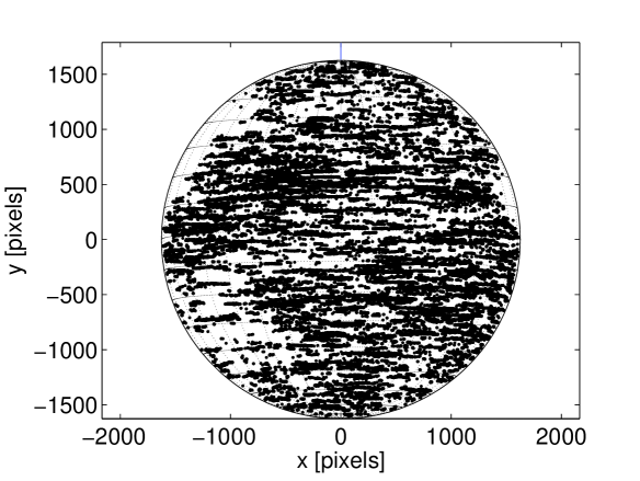
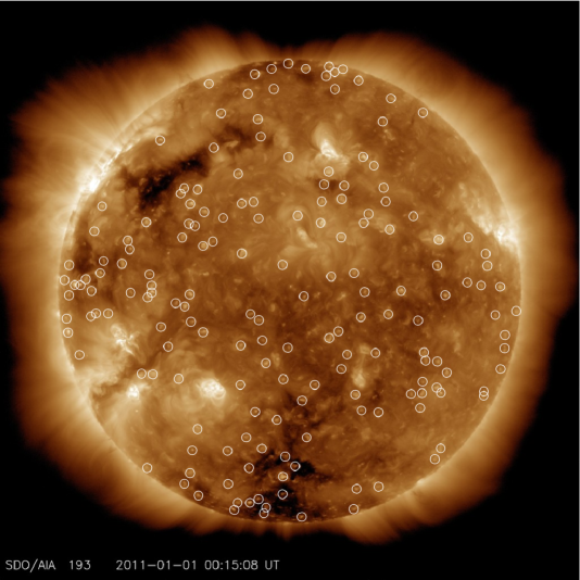
Figure 1: Distribution of CBPs detected by the segmentation algorithm (top panel) and image of the Sun in the 19.3 nm channel obtained by SDO/AIA on 1st of January 2011. White circles show detected CBPs on this image (bottom panel).

In top panel of Fig. 1 we show the distribution of detected CBPs and compare it to the full disk image of the Sun in the 19.3 nm channel obtained on 1st of January 2011 (bottom panel of the same Figure). In the bottom panel, white circles show CBPs that were detected on one image by the segmentation algorithm. We can see that CBPs are scarce in active regions, partly because of difficulties in detecting them against such bright and variable backgrounds.

The segmentation algorithm provides coordinates in pixels (centroids of CBPs on the image) and we converted them to heliographic coordinates taking into account the current solar distance given in FITS files (Roša et al. 1995, 1998). Positions of objects near the solar limb are fairly inaccurate. Limiting the data to $\pm$58°from the centre of the Sun or $\approx$0.85$R_{\odot}$ of the projected solar disk removes this problem (cf. Stark & Wöhl 1981; Balthasar et al. 1986a).

Figure 2: Motion of a single CBP. Top panel: latitude, $b$, over time, $t$; bottom panel: central meridional distance, $CMD$ over time, $t$.

As can be seen from Fig. 2, the calculated velocities show some scatter. This scatter arises because the shifts are fairly small at our 10 min cadence, and there can be significant variations in brightness and structure of CBPs which influences calculation of the centroid points. Nevertheless, trends are visible, especially in azimuthal motion which is known to be a significantly larger effect. The dominant azimuthal motion led us to approximate the CBP motion with a linear fit to calculate the velocities:

$$\omega_{syn}=\frac{N\sum\limits^{N}_{i=1}l_{i}t_{i}-\sum\limits^{N}_{i=1}l_{i}\sum\limits^{N}_{i=1}t_{i}}{N\sum\limits^{N}_{i=1}t^{2}_{i}-\left(\sum\limits^{N}_{i=1}t_{i}\right)^{2}},$$ (1)

$$\omega_{mer}=\frac{N\sum\limits^{N}_{i=1}b_{i}t_{i}-\sum\limits^{N}_{i=1}b_{i}\sum\limits^{N}_{i=1}t_{i}}{N\sum\limits^{N}_{i=1}t^{2}_{i}-\left(\sum\limits^{N}_{i=1}t_{i}\right)^{2}},$$ (2)

where $\omega_{syn}$ is a synodic rotational velocity, $\omega_{mer}$ is a meridional angular velocity, $l_{i}$ is central meridian distance (CMD) and $b_{i}$ is latitude of each measurement for a single CBP. We have also removed all CBPs which had less than 10 measurements of position in order for linear fits to be more robust. This is equivalent to 100 minutes or about 1°at the equator. To obtain the true rotation of CBPs on the Sun we convert synodic velocities to sidereal using Eq. 7 from Skokić et al. (2014).

Trying to identify the same object on subsequent images with an automatic method is bound to result in some misidentification. The resulting velocities are usually very large and can easily be removed by applying a simple velocity filter. Even the human factor can introduce such errors. For example, Sudar et al. (2014) analysed solar rotation residuals and meridional motions of sunspot groups from the Greenwich Photoheliographic Results and found that they had to use a filter 8$<\omega_{rot}<$19°day^-1 for rotational velocity in order to eliminate these erroneous measurements. The Greenwich Photoheliographic Results catalogue is being investigated and revised partly in order to remove such problems (Willis et al. 2013a, b; Erwin et al. 2013). In this work we have also used a 8$<\omega_{rot}<$19°day^-1 filter for rotational velocities to remove such outliers. In addition, we applied a meridional velocity filter of -4$<\omega_{mer}<$4°day^-1 to remove further outliers.

After completing all the procedures described above, we obtained 906 velocity measurements by tracing CBPs over just two days. Olemskoy & Kitchatinov (2005) pointed out that non-uniform distribution of tracers can result in false flows. This effect is most notable for meridional motion and rotation velocity residuals, but can easily be removed by assigning the calculated velocity to the latitude of the first measurement of position (Olemskoy & Kitchatinov 2005; Sudar et al. 2014). Although the effect is negligible for solar rotation, we nevertheless applied the correction in this work.

It is important to keep in mind that even when the tracers are uniformly distributed over the solar surface, the distribution of tracers in latitude will be non-uniform. As we move from equator to the pole, the area of each latitude bin becomes smaller, so we observe progressively fewer tracers ($\sim\cos{b}$).

3 Results

In this work, we present an analysis of the motion of CBPs observed by the SDO/AIA instrument. For a better understanding of the results and the potential of future studies along these lines, it is very useful to analyse the accuracy and errors of the dataset.

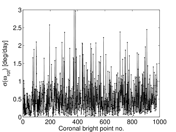
Figure 3: Errors of rotational velocity, $\sigma(\omega_{rot})$, for each of the 906 measurements.

In Fig. 3 we show errors of the calculated rotational velocities, $\sigma(\omega_{rot})$, for each CBP, which resulted from errors in the linear fitting of longitude vs time measurements. Although the errors can go up to 3°day^-1, the majority is below 1°day^-1. In Fig. 4 we show these errors in heliographic coordinates to check their spatial distribution on the solar surface.

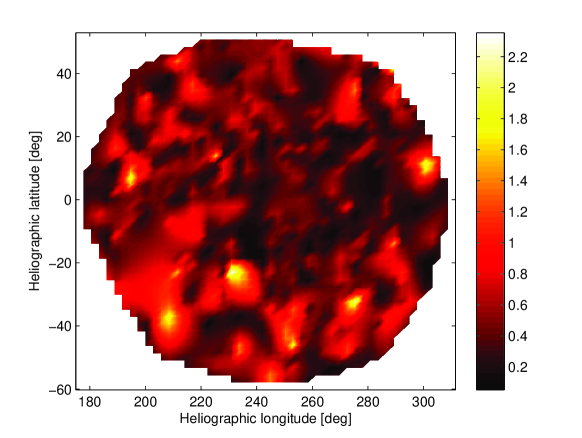
Figure 4: Distribution of rotation velocity errors ($\omega_{rot}$) in heliographic coordinates. Error scale is in ° day^-1.

Larger errors are shown with brighter shades and we can see that these roughly correspond to the positions of active regions shown in the bottom panel of Fig. 1. This correlation with active region is probably a consequence of the detection algorithm design and difficulties in detection of CBPs over a bright, variable background.

In Fig. 5 we show the distribution of CBPs in heliographic coordinates with arrows indicating the velocity vector.

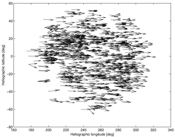
Figure 5: Distribution of CBPs in heliographic coordinates with arrows showing the direction and strength of the velocity vector.

As expected, the dominant effect is that of solar rotation.

The latitudinal dependence of rotational velocity is usually expressed as (Howard & Harvey 1970; Schröter 1985):

$$\omega_{rot}(b)=A+B\sin^{2}{b}+C\sin^{4}{b},$$ (3)

where $b$ is the latitude. Parameter $A$ represents equatorial velocity, while $B$ and $C$ depict the deviation from rigid body rotation. The problem with Eq. 3 is that the functions in this expression are not orthogonal, so the parameters are not independent of each other (Duvall & Svalgaard 1978; Snodgrass 1984; Snodgrass & Howard 1985; Snodgrass & Ulrich 1990). This crosstalk among the coefficients is particularity bad for $B$ and $C$. The effect of crosstalk does not affect the actual shape of the fit ($\omega_{rot}(b)$), but it creates confusion when directly comparing coefficients from different authors or obtained by different indicators.

There are various methods to alleviate this problem. Frequently $C$ is set to zero since its effect is noticeable only at higher latitudes. This is almost a standard practise when observing rotation by tracing sunspots or sunspot groups because their positions do not extend to high latitudes (Howard et al. 1984; Balthasar et al. 1986b; Pulkkinen & Tuominen 1998; Brajša et al. 2002a; Sudar et al. 2014).

Another method to reduce the crosstalk problem is to set the $C/B$ ratio to some fixed value. Scherrer et al. (1980) set the ratio $C/B=1$ while Ulrich et al. (1988), after measuring the covariance of $B$ and $C$, set the ratio to $C/B=1.0216295$.

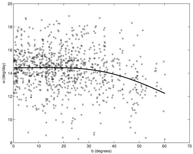
Figure 6: Solar differential rotation profile obtained with data from SDO/AIA. Open circles are individual measurements, while the solid line is the best fit defined by Eq. 3 for the $A\neq B\neq C$ case.

In Fig. 6 we show individual measurements of rotational velocities, $\omega_{rot}$, with respect to latitude, $b$, as open circles. We indicate, with a solid line, the best fit to the data using a functional form given in Eq. 3. Coefficients of the fit are given in Table 1. We also fitted the rotation profile for Northern and Southern solar hemisphere separately because of possible asymmetry (cf.eg. Wöhl et al. 2010) and show the results in the same table. Coefficient $A$ shows a larger value in the Southern hemisphere for all 3 fit functions. Jurdana-Šepić et al. (2011) reported that coefficient $A$ is larger when solar activity is smaller. According to the SIDC data (SILSO World Data Center 2011) we can see that Northern hemisphere is more active both when looking at the monthly smoothed means and daily sunspot data, consistent with Jurdana-Šepić et al. (2011). However, judging by the errors of the coefficients, the difference between South and North is statistically low and the hypothesis that this is a result of asymmetric solar activity needs to be verified with a larger data sample.

Table 1: Coefficients of the solar rotation profile.

Type	$A$ [°day-1]	$B$ [°day-1]	$C$ [°day-1]	$n$
$A$, $B$, $C$	14.47$\pm$0.10	+0.6$\pm$1.0	-4.7$\pm$1.7	906
$A$, $B=C$	14.59$\pm$0.07	-1.35$\pm$0.21	-1.35$\pm$0.21	906
$A$, $B$, $C=0$	14.62$\pm$0.08	-2.02$\pm$0.33	0	906
Northern hemisphere
$A$, $B$, $C$	14.43$\pm$0.13	+0.8$\pm$1.5	-5.6$\pm$3.0	461
$A$, $B=C$	14.55$\pm$0.10	-1.35$\pm$0.35	-1.35$\pm$0.35	461
$A$, $B$, $C=0$	14.57$\pm$0.10	-1.92$\pm$0.52	0	461
Southern hemisphere
$A$, $B$, $C$	14.50$\pm$0.15	+0.7$\pm$1.4	-4.8$\pm$2.3	445
$A$, $B=C$	14.65$\pm$0.11	-1.39$\pm$0.28	-1.39$\pm$0.28	445
$A$, $B$, $C=0$	14.69$\pm$0.12	-2.14$\pm$0.45	0	445

In Fig. 7 we show a comparison between different fitting techniques: $A\neq B\neq C$ (solid line), $A\neq B=C$ (dashed line) and $A\neq B$, $C=0$ (dotted line). In the same figure we also show average values of $\omega_{rot}$ in bins 5° wide in latitude, $b$, with their respective errors.

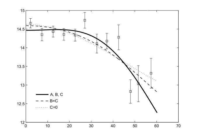
Figure 7: Comparison of three different fitting procedures for the solar differential rotation profile. Average values of $\omega_{rot}$ in 5° bins in latitude, $b$, are also shown with their respective errors.

4 Discussion

Table 2: Comparison with some other results.

Method/object	time period	$A$ [°day-1]	$B$ [°day-1]	$C$ [°day-1]	$A_{G}$ [°day-1]	$B_{G}$ [°day-1]	$C_{G}$ [°day-1]	Ref
CBPs	1967	14.65$\pm$0.2			14.65			(1)
CBPs	1994-1997	14.39$\pm$0.01	-1.91$\pm$0.10	-2.45$\pm$0.17	13.80	-0.709	-0.117	(2)
CBPs	1998-1999	14.454$\pm$0.027	-2.22$\pm$0.07	-2.22$\pm$0.07	13.82	-0.740	-0.106	(3)
CBPs	1998-2006	14.499$\pm$0.006	-2.54$\pm$0.06	-0.77$\pm$0.09	13.93	-0.611	-0.037	(4)
CBPs	1-2 Jan 2011	14.47$\pm$0.10	+0.6$\pm$1.0	-4.7$\pm$1.7	14.19	-0.507	-0.224	(5)
CBPs	1-2 Jan 2011	14.59$\pm$0.07	-1.35$\pm$0.21	-1.35$\pm$0.21	14.20	-0.450	-0.064	(5)
CBPs	1-2 Jan 2011	14.62$\pm$0.08	-2.02$\pm$0.33		14.22	-0.404		(5)
sunspot groups	1853-1996	14.531$\pm$0.003	-2.75$\pm$0.05		13.98	-0.550		(6)
sunspot groups	1874-1976	14.551$\pm$0.006	-2.87$\pm$0.06		13.98	-0.574		(7)
sunspot groups	1878-2011	14.499$\pm$0.005	-2.64$\pm$0.05		13.97	-0.528		(8)
sunspot groups	1880-1976	14.37$\pm$0.01	-2.59$\pm$0.16		13.85	-0.518		(9)
sunspots	1921-1982	14.522$\pm$0.004	-2.84$\pm$0.04		13.95	-0.568		(10)
sunspot groups	1921-1982	14.393$\pm$0.010	-2.95$\pm$0.09		13.80	-0.590		(10)
H$\alpha$ filaments	1972-1987	14.45$\pm$0.15	-0.11$\pm$0.90	-3.69$\pm$0.90	14.11	-0.514	-0.176	(11)
magnetic features	1967-1980	14.307$\pm$0.005	-1.98$\pm$0.06	-2.15$\pm$0.11	13.73	-0.683	-0.102	(12)
magnetic features	1975-1991	14.42$\pm$0.02	-2.00$\pm$0.13	-2.09$\pm$0.15	13.84	-0.679	-0.100	(13)
Doppler	1966-1968	13.76	-1.74	-2.19	13.22	-0.640	-0.104	(14)
Doppler	1967-1984	14.05	-1.49	-2.61	13.53	-0.646	-0.124	(15)
Helioseismology	1996	14.16	-1.63	-2.52	13.62	-0.662	-0.120	(16)
Helioseismology	Apr 2002	14.04	-1.70	-2.49	13.49	-0.672	-0.119	(17)

(1) Dupree & Henze (1972); (2) Hara (2009); (3) Brajša et al. (2004); (4) Wöhl et al. (2010); (5) this paper; (6) Pulkkinen & Tuominen (1998); (7) Balthasar et al. (1986b); (8) Sudar et al. (2014); (9) Brajša et al. (2002a); (10) Howard et al. (1984) (11) Brajša et al. (1991); (12) Snodgrass (1983); (13) Komm et al. (1993); (14) Howard & Harvey (1970); (15) Snodgrass (1984); (16) Schou et al. (1998); (17) Komm et al. (2004)

In Table 2 we show a comparison of the solar differential profile (Eq. 3) from a number of different sources, including the results from this paper (Table 1). Since we found no statistically significant difference between Northern and Southern hemisphere we only include the results for both hemispheres combined. Results in Table 2 come from a wide variety of different techniques, tracers and instruments.

Snodgrass (1984) suggested that the rotation profile should be expressed in terms of Gegenbauer polynomials since they are orthogonal on the disk. This eliminates the cross-talk problem between coefficients in Eq. 3. Using the expansion in terms of Gegenbauer polynomials solar rotation profile becomes:

$$\omega_{rot}(b)=A_{G}T_{0}^{1}(\sin b)+B_{G}T_{2}^{1}(\sin b)+C_{G}T_{4}^{1}(\sin b),$$ (4)

where $A_{G}$, $B_{G}$ and $C_{G}$ are coefficients of expansion and $T_{0}^{1}(\sin b)$, $T_{2}^{1}(\sin b)$ and $T_{4}^{1}(\sin b)$ are Gegenbauer polynomials as defined by Snodgrass & Howard (1985) in their equation (2).

As Snodgrass & Howard (1985); Snodgrass & Ulrich (1990) pointed out, the relationship between coefficients $A$, $B$ and $C$ from standard rotation profile (Eq. 3) and coefficients $A_{G}$, $B_{G}$ and $C_{G}$ from Eq. 4 is linear. Therefore, it is not necessary to recalculate the fits using Gegenbauer polynomials, we can compute $A_{G}$, $B_{G}$ and $C_{G}$ directly from $A$, $B$ and $C$. We used the relationship given in Snodgrass & Howard (1985) (their equation (4)) since there seems to be a typo for a similar relationship for coefficients $C$ and $C_{G}$ in Snodgrass & Ulrich (1990). In Table 2 we also show the values of coefficients $A_{G}$, $B_{G}$ and $C_{G}$.

Our rotational profile results are roughly consistent with all the previously published work we surveyed (Table 2). The accuracy of our coefficients is lower when compared with other results, a consequence of our fairly small number of data points ($n=906$). Wöhl et al. (2010), for example, had more than 50000 data points spanning a time interval of 8 years. We have used data spanning only 2 days. It is therefore reasonable to expect that with AIA/SDO CBP data we could reach 50000 data points with only 4 months of data and achieve similar accuracy in solar rotation profile coefficients. This means that with AIA/SDO data it should be possible to measure rotation profile several times per year and track possible changes in solar surface differential rotation directly with a very simple tracer method. This is also true for meridional motion and Reynolds stress, both of which probably vary over the solar cycle (cf. e.g Sudar et al. 2014).

5 Summary and Conclusion

Using 19.3nm data from the SDO/AIA instrument at 10 min cadence we have identified a large number of CBPs, resulting in 906 rotation velocity measurements. We obtained a fairly good differential solar rotation profile in spite of the fact that we used data spanning only two days. The large density of data points in time is a result of several factors. The instrument itself (SDO/AIA) has better spatial resolution and is capable of high cadence ($<$5 min). For comparison, SOHO/EIT 28.4 nm channel had a cadence of two images every 6 hours (Wöhl et al. 2010). In this work, the high cadence enabled us to track and measure velocities of short lived CBPs which couldn’t be detected or accurately tracked by the comparatively large time interval between successive images in the SOHO/EIT 28.4 nm channel. Coupled with the fact that short lived CBPs are more numerous than long lived ones (Brajša et al. 2008), this resulted in a very high density of data points in time. High data density necessitated the use of an automatic procedure to detect and track CBPs. The segmentation algorithm used here proved to be completely adequate for the task, as similar algorithms have elsewhere (McIntosh & Gurman 2005; McIntosh et al. 2014a, b).

The surface rotation profile and its accuracy obtained by helioseismology is seldom given in a form suitable for comparison with those obtained by tracer measurements. We can estimate from the number of published significant digits in the results Schou et al. (1998); Komm et al. (2004), given in Table 2, that the accuracy is of the same order as better quality tracer measurements. Zaatri et al. (2009) published the error for the coefficient $B$ (see Eq. 3) and the value of 0.01 from that paper is in agreement with our estimate above.

It is quite conceivable that errors in the differential rotation profile coefficients would drop significantly when more data is used. From our analysis, we can expect to obtain 400-500 velocity measurements per day from CBPs using SDO/AIA. A time interval of 4 months seems adequate to obtain 50000 velocity measurements, which should be sufficient to match the most accurate results obtained by tracer methods (for example Wöhl et al. (2010)).

CBPs are also very good tracers since they extend to much higher latitudes than sunspots. They are also quite numerous in all phases of the solar cycle while sunspots are often absent in the minimum of the cycle.

This opens up an intriguing possibility of measuring the solar rotation profile almost from one month to the next over an entire cycle. Such studies could provide new insight into mechanisms responsible for solar rotation. We already know that meridional motion exhibits some changes during the course of the solar cycle, and the same is probably true for Reynolds stress. Sudar et al. (2014) found by averaging almost 150 years of sunspot data that meridional motion changes slightly over the solar cycle and hinted that the Reynolds stresses are probably changing too. Here we have found a small asymmetry in rotation profile for two solar hemispheres and suggested that this might be related to different solar activity levels in the two hemispheres. This needs to be verified with a larger dataset though, as the difference in rotation profiles was of low statistical significance.

The planned SDO mission duration of 5–10 years will cover a large portion of the solar cycle which should result in enormous amount of velocity data to assist in the understanding of the nature and variation of solar rotation profile. Having more detailed temporal resolution and direct results (without the need to average many solar cycles) could prove to be very informative.

A time interval of 10 minutes between successive images also offers a good opportunity to study the evolution of CBPs and possible effect this might have on the detected surface velocity fields. For example, Vršnak et al. (2003) reported that longer lasting CBPs show different results than short-lived CBPs.

Based on the promising results here, we will use larger datasets to further exploit the potential of SDO/AIA CBP data to determine meridional motions, rotation velocity residuals, Reynolds stresses and proper motions in subsequent papers.