Hastatic Order in URu₂Si₂ : Hybridization with a Twist

Abstract

The broken symmetry that develops below 17.5K in the heavy fermion compound URu₂Si₂ has long eluded identification. Here we argue that the recent observation of Ising quasiparticles in URu₂Si₂ results from a spinor hybridization order parameter that breaks double time-reversal symmetry by mixing states of integer and half-integer spin. Such “hastatic order” (hasta:[Latin]spear ) hybridizes Kramers conduction electrons with Ising, non-Kramers $5f^{2}$ states of the uranium atoms to produce Ising quasiparticles. The development of a spinorial hybridization at 17.5K accounts for both the large entropy of condensation and the magnetic anomaly observed in torque magnetometry. This paper develops the theory of hastatic order in detail, providing the mathematical development of its key concepts. Hastatic order predicts a tiny transverse moment in the conduction sea, a collosal Ising anisotropy in the nonlinear susceptibility anomaly and a resonant energy-dependent nematicity in the tunneling density of states.

I Introduction

The heavy fermion superconductor URu₂Si₂ exhibits a large specific heat anomaly at $T_{0}=$17.5K signalling the development of long-range order with an associated entropy of condensation, $\int_{0}^{T_{0}}\frac{C_{V}}{T}dT\approx\frac{1}{2}R\ln 2$ per mole formula unitPalstra85 ; Schlabitz86 . This sizable ordering entropy in conjunction with the sharpness of the specific heat anomaly suggests underlying itinerant ordering; however the anisotropic bulk spin susceptibility (cf. Fig. 1) of URu₂Si₂ displays Curie-Weiss behavior down to $T\sim 70K$ indicative of local moment behavior. Initially, the hidden order was attributed to a spin density wave with a tiny c-axis momentbroholm91 ; walter93 , which was later shown to be extrinsictakagi07 . However, spin ordering in the form of antiferromagnetism is observed at pressures exceeding 0.8GPaAmitsuka99 ; Amitsuka07 ; Butch2010 . Despite thirty years of intense experimental effort, no laboratory probe has yet coupled directly to the order parameter in URu₂Si₂ at ambient pressure, though there have been a wide variety of theoretical proposals for this “hidden order” (HO) problemAmitsuka94 ; Haule09 ; Santini94 ; Varma ; pepin ; Morr10 ; Dubi10 ; Fujimoto11 ; Ikeda11 ; Mydosh11 ; hastatic ; Flint14 ; Chandra14 . We point the interested reader to a recent review on URu₂Si₂ for more details.Mydosh11

Expanding on our recent proposalhastatic ; Flint14 ; Chandra14 of “hastatic order” in URu₂Si₂ , here we argue that the failure to observe the nature of its “hidden order” is not due to its intrinsic complexity but instead results from a fundamentally new kind of broken time-reversal symmetry associated with an order parameter of spinorial, half-integer spin character. Key evidence supporting this conjecture is the observation of quasiparticles with an Ising anisotropy characteristic of integer spin f-momentsOhkuni99 ; Altarawneh11 ; Hc2 ; Altarawneh2 . Hastatic order accounts for this unusual feature as a consequence of a spinor order parameter that coherently hybridizes the integer spin, Ising f-moments with half-integer spin conduction electrons; the observed quasiparticle and the magnetic anisotropies thus have the same origin.

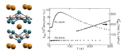
Figure 1: (a) Tetragonal structure of URu₂Si₂ (b) Temperature dependence of magnetic susceptibility in URu₂Si₂ after palstra86 .

I.1 Experimental Motivation for Hastatic Order

Above the hidden order transition, URu₂Si₂ is an incoherent heavy fermion metal, with an large, anisotropic, linear resistivitypalstra86 ,and a linear specific heat with $\gamma=\frac{C_{V}}{T}\sim 200$mJmol^-1K^-2 . The development of hidden order results in a significant reduction in the specific heat to $\gamma_{0}=\frac{C_{V}}{T}\sim 60$ mJmol^-1K^-2, corresponding to the the loss of about two-thirds of the heavy Fermi surfaceMydosh11 . At $T_{c}=1.5K$, the remaining heavy quasiparticles go superconducting. Under a modest pressure of 0.8GPa, the hidden order ground-state of URu₂Si₂ undergoes a first order transition into an Ising antiferromagnet with an staggered ordered moment of order 0.4 $\mu_{B}$ aligned along the c-axisAmitsuka07 . de Haas-van Alphen (dHvA) shows that the quasiparticles in the hidden order phase form small, highly coherent heavy electron pockets with an effective mass up to $8.5m_{e}$Ohkuni99 . Remarkably, these small heavy electron pockets survive across the first order transition into the high-pressure antiferromagnetic phase, leading many groups to conclude that the (commensurate) ordering wavevectors ${\bf Q}=(0,0,1)$ of the antiferromagnetic and the HO phases are the sameJo07 ; Villaume08 ; Hassinger10 ; Haule09 ; Haule10 .

Perhaps the most dramatic feature of these heavy electron pockets is the essentially perfect Ising magnetic anisotropy in the magnetic g-factors of the itinerant heavy f-electrons in the HO state of URSAltarawneh11 . This Ising quasiparticle anisotropy has been determined by measuring the Fermi surface magnetization in an angle-dependent magnetic field in the HO state; this magnetization is a periodic function of the ratio of the Zeeman and the cyclotron energies, where the former is defined through an angle-dependent g-factor $g(\theta)$

$$\Delta E(\theta)=g(\theta)\mu_{B}|B|.$$ (1)

Interference of Zeeman-split orbits in tilted fields leads to spin zeroes in the quantum oscillation measurements (cf. Fig. 2) satisfying the condition

$$g(\theta_{n})\frac{m^{*}}{m_{e}}=2n+1$$ (2)

where $n$ is a positive integer and $\theta_{n}$ is the (indexed) angle with respect to the c-axis. Sixteen such spin zeroes were identified in the HO state of URSOhkuni99 ; Altarawneh11 , and the experimentalists found that

$$\frac{g_{\perp}}{g_{c}}<\frac{1}{30}$$ (3)

where $g_{\perp}=g(\theta_{n}\sim\frac{\pi}{2})$ and $g_{c}=g(\theta_{n}=0)$, indicating that $\Delta E(\theta_{n})$ depends solely on the c-axis component of the applied magnetic field ($B_{c}$), namely that

$$g(\theta_{n})=g^{*}\cos\theta_{n}$$ (4)

where $g^{*}=2.6$ in contrast to the isotropic $g=2$ for free electrons.

In these high-field measurements, the quasiparticle anisotropy manifests itself through the appearance of a rapid modulation in the amplitude of the dHvA oscillations generated by the heavy $\alpha$ pockets of URu₂Si₂ as the magnetic field is tilted from the c-axis into the basal plane. The same magnetic anisotropy is also observed in the angular dependence of the upper-critical field of the superconducting state which develops at low temperatures (cf. Fig. 2)Hc2 ; Altarawneh2 . Whereas the dHvA measurements could in principle belong to a select region of the Fermi surface, the upper-critical field, $H_{c2}(\theta)$ is sensitive to the entire heavy fermion pair condensate, proving crucially that the Ising quasiparticle anisotropy pervades the entire Fermi surface of hidden order state. We note that while $H_{c2}(\theta)$ matches the anisotropy of the g-factor for angles near the c-axis, where $H_{c2}$ is Pauli limited, when the field is in-plane, $H_{c2}(\theta)$ is larger than expected, likely due to orbital contributions. We note that since the Pauli susceptibility $\chi^{P}$ scales with the square of the g-factor, these resolution-limited measurements of $\frac{g_{c}}{g_{\perp}}$ suggest that

$$\chi^{P}(\theta)=\chi^{P*}\cos^{2}\theta\qquad\frac{\chi^{P}_{c}}{\chi^{P}_{\perp}}>900.$$ (5)

Such a large anisotropy should be observable in electron spin resonance measurements that probe the Pauli susceptibility directly in contrast to bulk susceptibility measurements where Van Vleck contributions are also present.

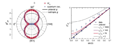
Figure 2: (a) Anisotropy of the measured g-factorAltarawneh11 plotted (a) in polar co-ordinates derived from spin zeros in quantum oscillation measurements and the anisotropy of the upper critical field (b) versus sine of the angle out of the basal plane, showing that the dataAltarawneh11 requires a Pauli susceptibility anisotropy in excess of a thousand.

I.2 Ground-State Configuration of the Uranium Ion

Bulk susceptibility measurements (see Fig. 1) of URu₂Si₂ reveal that the magnetic U ions have an Ising anisotropy, with a magnetic moment that is consistent either with a U³⁺ ($5f^{3}$) configuration or a non-Kramers $U^{4+}$ ($5f^{2}$) ionPalstra85 ; Ramirez92 . A natural explanation for the quasiparticle Ising anisotropy is that the Ising character of the uranium (U) ions has been transferred to the quasiparticles via hybridization, and this is a key element of the hastatic proposal. The giant anisotropy in $\frac{g_{\perp}}{g_{c}}$, places a strong constraint on the energy-splitting $\Delta$ between the two Ising states

$$\frac{2\Delta}{(g_{c}\mu_{B}B_{\rm dHvA})}<\frac{1}{30}$$ (6)

requiring that in a transverse field, $B_{\rm dHvA}=11\rm{T}$ the U ion is doubly degenerate to within $\Delta\sim 1K$. Further support for a very small $\Delta$ comes from the dilute limit, U_xTh_1−xRu₂Si₂ ($x\leq.07$), where the Curie-like single-ion behavior crosses over to a critical logarithmic temperature-dependenceAmitsuka94 below $10K$, $−\log T/T_{K}$, where $T_{K}\approx 10K$. This physics has been attributed to two channel Kondo criticality, again requiring a splitting $\Delta\ll 10K$. Such a degeneracy is of course natural for in a Kramers U ($5f^{3}$) ion, containing an odd-number of f-electrons. However it can also occur in a $5f^{2}$ “non-Kramers doublet” with a two-fold orbital degeneracy protected by tetragonal symmetryAmitsuka94 ; Ohkawa99 .

Motivated and constrained by the bulk spin susceptibility and the quantum spin zeroes, we therefore require the U ion to be in an Ising doublet in the tetragonal environment of URS (cf. Fig. 1); such a magnetic doublet of URu₂Si₂ has the form

$$|\Gamma_{\pm}\rangle=\sum_{n}a_{n}|\pm(J_{z}-4n)\rangle,$$ (7)

where the addition and subtraction of angular momentum in units of $4\hbar$ is a consequence of the four-fold symmetry of the tetragonal crystal. However, the presence of a perfect Ising anisotropy requires an Ising selection rule

$$\langle\Gamma_{\pm}|J_{\pm}|\Gamma_{\mp}\rangle=0$$ (8)

that, in the absence of fine-tuning of the coefficients $a_{n}$, leads to the condition that $-(J_{z}+4n^{\prime})\neq(J_{z}+4n)\pm 1$, or $J_{z}\neq 2(n-n^{\prime})\pm\frac{1}{2}$, requiring $J_{z}\in\mathbb{Z}$ must be an integer. For any half-integer $J_{z}$, corresponding to a Kramers doublet, the selection rule is absent and the ion will develop a generic basal-plane moment. As an aside we note that the fine-tuned case will produce an Ising Kramers doublet, but corresponds to the complete absence of tetragonal mixing, highly unlikely in a tetragonal environment.

Let us apply this argument specifically to the case of URu₂Si₂ . We first suppose that the U ion is in a $5f^{3}$ ($J=\frac{9}{2}$) configuration, predominantly in a $|\pm\frac{7}{2}\rangle$ state. The presence of tetragonal symmetry results in a crystal-field ground-state

$$|\pm\rangle=a|\pm\frac{7}{2}\rangle+b|\mp\frac{1}{2}\rangle+c|\mp\frac{9}{2}\rangle$$ (9)

so that $|\langle-|J_{+}|+\rangle|^{2}=5b^{2}+6ac$ and perfect Ising anisotropy is only achieved with fine-tuning of the tetragonal mixing coefficients such that the condition $5b^{2}+6ac=0$ is satisfied. By contrast, for U ion in a $5f^{2}$ ($J=4$) configuration, its ground-state may be a non-Kramers $\Gamma_{5}$ doublet

$$|\pm\rangle=a|\pm 3\rangle+b|\mp 1\rangle,$$ (10)

where Ising anisotropy exists for arbitrary mixing between the $|\pm 3\rangle$ and $|\mp 1\rangle$ states since this tetragonally-stabilized $\Gamma_{5}$ state is dipolar in the c-direction and quadrupolar in the a-b plane. Because the phase space associated with the non-Kramers doublet is significantly larger than that for its finely-tuned Kramers counterpart, we take the $\Gamma_{5}$ doublet to be the more natural ground-state configuration of the U ion in URS. However we have proposed a direct benchtop test to distinguish between these two single-ion U ground-state configurations in URu₂Si₂ using the basal-plane nonlinear susceptibility to check this key assumption in the hastatic proposalflint12 .

The combination of the observed Ising anisotropy and tetragonal symmetry are crucial towards pointing us to the non-Kramers $\Gamma_{5}$ doublet. By contrast in a hexagonal system, like CeAl₃Goremychkin00 , the six-fold symmetry mixes terms that differ by $6\hbar$ units of angular momentum, so a pure doublet $|\pm M\rangle$ mixes with $|\pm M^{\prime}\rangle$ states only if $M^{\prime}=M-6n\;(n\in\mathbb{Z})$. For $J<7/2$, the maximum $M-M^{\prime}$ is $\frac{5}{2}-(-\frac{5}{2})=5$ meaning there is no valid choice of $M$ and $M^{\prime}$; thus there are two Ising doublets for the Ce ($J=5/2$) case: $|\pm 5/2\rangle$ and $|\pm 3/2\rangle$. These Kramers doublets can undergo a single channel Ising Kondo effect Goremychkin00 ; sikkema96 that will differ substantially from the two-channel Kondo physics associated with a non-Kramers doubletCoxZawad .

I.3 Hybridization, Hastatic Order and Double-Time Reversal Symmetry

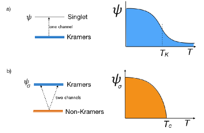
Figure 3: Schematic of (a) conventional (scalar) vs (b) spinorial hybridization where the hybridization is a) a crossover and b) breaks spin-rotational and time-reversal symmetries and thus develops discontinuously as a phase transition.

The formation of heavy f-bands in heavy fermion systems involves the formation of f-resonances within the conduction sea. Hybridization between these many-body resonances and the conduction electrons produces charged heavy f-electrons that inherit the magnetic properties of the local moments. When this process involves a Kramers doublet (the usual case), the hybridization can develop without any broken symmetry and thus is associated with a crossover. At first sight, the most straightforward explanation of hidden order is to attribute it to the formation of a “heavy density wave” within a pre-formed heavy electron fluid. Since there is no observed magnetic moment or charge density observed in the hidden order phase, such a density wave must necessarily involve a higher order multipole of the charge or spin degrees of freedom and various theories in this category have indeed been advanced. In each of these scenarios, the heavy electrons develop coherence via cross-over at higher temperatures, and the essential hidden order is then a multipolar charge or spin density wave. However such multipolar order can not account for the emergence of heavy Ising quasiparticles. The essential point here, is that conventional quasiparticles have half-integer spin, lacking the lack the essential Ising protection required by experiment.

Moreover, in URu₂Si₂ both optical Timusk11 and tunnelling Schmidt10 ; Aynajian10 ; Park11 probes suggest that hybridization develops abruptly at the HO transition, leading to proposalsMorr10 ; Dubi10 that the hybridization is an order parameter. The associated global broken symmetry and phase transition is naturally described within the hastatic proposal. As we now describe, hybridization with a non-Kramers doublet requires the development of an order parameter that breaks double time-reversal symmetry, a requirement that leads us to conclude that the order parameter has a spinorial quality. (See Fig. 3)

The observation of heavy quasiparticles with Ising anisotropy in the tetragonal environment of URS implies an underlying hybridization of half-integer spin electrons with integer-spin doublets that has important symmetry implications for the nature of the hidden order. More specifically such hybridization requires a quasiparticle mixing terms in the low-energy fixed-point Hamiltonian of the form

$${\cal H}=|k\sigma\rangle V_{\sigma\alpha}(k)\langle\alpha|+H.C.$$ (11)

where $|k\sigma\rangle$ and $|\alpha\rangle$ refer to the half-integer spin conduction and the integer-spin doublet states respectively and H.C. is the Hermitian conjugate; here $k$ and $\sigma$ are the momentum and the spin components respectively. Because time-reversal, $\hat{\Theta}$, is an anti-unitary quantum operator, it has no associated eigenvalue. However double time-reversal $\hat{\Theta}^{2}$, equivalent to a $2\pi$ rotation, is a unitary operator whose quantum number is the Kramers index, $K=(-1)^{2J}$ where $J$ refers to the total angular momentum of the quantum state; $K$ defines the phase factor acquired by its wavefunction after two successive time-reversals:

$$\hat{\Theta}^{2}|\psi\rangle=|\psi^{2\pi}\rangle=K|\psi\rangle.$$ (12)

For an integer-spin state $|\alpha\rangle$, $K=1$ since $|\alpha^{2\pi}\rangle=+|\alpha\rangle$, indicating that it is unchanged by a $2\pi$ rotation. By contrast, for conduction electrons with half-integer spin states, $|k\sigma\rangle$, $|k\sigma^{2\pi}\rangle=-|k\sigma\rangle$, so that $K=-1$. Therefore, by mixing half-integer and integer spin states, the quasiparticle hybridization ${\cal H}$ does not conserve Kramers index. Indeed application of two successive time-reversals to ${\cal H}$ yields

$$\hat{\Theta}^{2}(V|k\sigma\rangle\langle\alpha|)=V^{{2\pi}}|k\sigma^{2\pi}\rangle\langle\alpha^{2\pi}|=-V^{2\pi}|k\sigma\rangle\langle\alpha|.$$ (13)

Since the microscopic Hamiltonian must be time-reversal invariant, it follows that

$$V=-V^{2\pi}$$ (14)

so the hybridization transforms as a half-integer spin state and is therefore a spinor. It then follows that this spinorial hybridization breaks both single- and double-time reversal symmetries distinct from conventional magnetism where Kramers index is conserved; we call this new state of matter “hastatic (Latin: spear) order”.

Before we proceed to discuss the theory of spinorial hybridization and its consequences, let us pause briefly to elaborate on the distinction between spinors and vectors, expanding the previous discussion with emphasis on time-reversal symmetry properties. Quantum mechanically, the non-relativistic evolution of a wavefunction $\psi(x,t)$ is described by the Schrödinger equation $H\psi=i\hbar\frac{\partial\psi}{\partial t}$ so that

$$\Theta\psi(x,t)=\psi^{*}(x,-t)$$ (15)

where $\Theta$ is the time-reversal operator; this is an anti-unitary operation. For vector spins, $\vec{S}\rightarrow-\vec{S}$. The spin $\frac{1}{2}$ wavefunction is a spinor

$$\Psi=\left(\begin{matrix}\psi_{\uparrow}\cr\psi_{\downarrow}\end{matrix}\right)$$ (16)

so that

$$\Theta\Psi(x,t)=\left(\begin{matrix}-\psi^{*}_{\downarrow}(x,-t)\cr\psi^{*}_{\uparrow}(x,-t)\end{matrix}\right)$$ (17)

and

$$\Theta^{2}\Psi(x,t)=\left(\begin{matrix}-\psi^{*}_{\uparrow}(x,t)\cr-\psi^{*}_{\downarrow}(x,t)\end{matrix}\right)=-\Psi(x,t)$$ (18)

Bosons, with integer spins, are vectors with $\Theta^{2}=+1$, whereas fermions with half-integer spins have $K=-1$. Because of its spinorial character, we can think of hastatic order as “hybridization with a twist” since this is a simple way of visualization its behavior under $2\pi$ (inverted) and $4\pi$ (restored) rotations.

Hybridization in heavy fermion compounds is usually driven by valence fluctuations mixing a ground-state Kramers doublet and an excited singlet (cf. Fig. 1a). In this case, the hybridization amplitude is a scalar that develops via a crossover, leading to mobile heavy fermions. However valence fluctuations from a $5f^{2}$ ground-state create excited states with an odd number of electrons and hence a Kramers degeneracy (cf. Fig. 1b). Then the quasiparticle hybridization has two components, ${\Psi}_{\sigma}$, that determine the mixing of the excited Kramers doublet into the ground-state. These two amplitudes form a spinor defining the “hastatic” order parameter

$${\Psi}=\left(\begin{matrix}{\Psi}_{\uparrow}\cr{\Psi}_{\downarrow}\end{matrix}\right).$$ (19)

Loosely speaking, the hastatic spinor is the square root of a multipole

$$\Psi\sim\sqrt{\hbox{multipole}}.$$ (20)

Moreover, the presence of distinct up/down hybridization components indicates that $\Psi$ carries a half-integer spin quantum number; its development must now break double time-reversal and spin rotational invariance via a phase transition.

Under pressure, URu₂Si₂ undergoes a first-order phase transition from the hidden order (HO) state to an antiferromagnet (AFM) Amitsuka07 . These two states are remarkably close in energy and share many key featuresJo07 ; Villaume08 ; Hassinger10 including common Fermi surface pockets; this motivated the recent proposal that despite the first order transition separating the two phases, they are linked by “adiabatic continuity,”Jo07 corresponding to a notional rotation of the HO in internal parameter space Haule09 ; Haule10 . In the magnetic phase, this spinor points along the c-axis

$${\Psi}_{A}\sim\left(\begin{matrix}1\cr 0\end{matrix}\right)\hbox{, }{\Psi}_{B}\sim\left(\begin{matrix}0\cr 1\end{matrix}\right)$$ (21)

corresponding to time-reversed configurations on alternating layers A and B, leading to a staggered Ising moment. For the HO state, the spinor points in the basal plane

$${\Psi}_{A}\sim\frac{1}{\sqrt{2}}\left(\begin{matrix}e^{-i\phi/2}\cr e^{i\phi/2}\end{matrix}\right)\hbox{, }{\Psi}_{B}\sim\frac{1}{\sqrt{2}}\left(\begin{matrix}-e^{-i\phi/2}\cr e^{i\phi/2}\end{matrix}\right),$$ (22)

where again, $\Psi_{B}=\Theta\Psi_{A}$. This state is protected from developing large moments by the pure Ising character of the $5f^{2}$ ground-state.

I.4 Two-Channel Valence Fluctuation Model

We next present a model that relates hastatic order to the particular valence fluctuations in URu₂Si₂, based on a two-channel Anderson lattice model. The uranium ground state is a $5f^{2}$ Ising $\Gamma_{5}$ doubletAmitsuka94 , which then fluctuates to an excited $5f^{3}$ or $5f^{1}$ state via valence fluctuations. The lowest lying excited state is most likely the $5f^{3}$ ($J=9/2$) state, but for simplicity here we take it to be the symmetry equivalent $5f^{1}$ state, and assume that fluctuations to the $5f^{3}$ are suppressed - in this sense, we take an infinite-U two-channel Anderson model.

As we can write the $f^{2}$ $\Gamma_{5}$ doublet, $|\pm\rangle=a|\pm 3\rangle+b|\mp 1\rangle$ in terms of combinations of two $J=5/2$ f-electrons in the three tetragonal orbitals, $\Gamma_{7}^{\pm}$ and $\Gamma_{6}$,

$$|+\rangle = ({p}f^{\dagger}_{\Gamma_{7}^{-}\downarrow}f^{\dagger}_{\Gamma_{7}^{+}\downarrow}+{q}f^{\dagger}_{\Gamma_{6}\uparrow}f^{\dagger}_{\Gamma_{7}^{+}\uparrow}+{s}f^{\dagger}_{\Gamma_{6}\uparrow}f^{\dagger}_{\Gamma_{7}^{-}\uparrow})|\Omega\rangle$$ (23)

$$|-\rangle = ({p}f^{\dagger}_{\Gamma_{7}^{-}\uparrow}f^{\dagger}_{\Gamma_{7}^{+}\uparrow}+{q}f^{\dagger}_{\Gamma_{6}\downarrow}f^{\dagger}_{\Gamma_{7}^{+}\downarrow}+{s}f^{\dagger}_{\Gamma_{6}\downarrow}f^{\dagger}_{\Gamma_{7}^{-}\downarrow})|\Omega\rangle,$$ (24)

if we assume a $5f^{1}$ $\Gamma_{7}^{+}$ excited state, we can now read off the valence fluctuation matrix elements directly. Valence fluctuations occur in two orthogonal conduction electron channels, $\Gamma_{7}^{-}$ and $\Gamma_{6}$, and we find

$$H_{VF}(j) = V_{6}{c}_{\Gamma_{6}\pm}^{\dagger}(j)|\Gamma_{7}^{+}\pm\rangle\langle\Gamma_{5}\pm|$$ (26)

$$+ V_{7}{c}_{\Gamma_{7}\mp}^{\dagger}(j)|\Gamma_{7}^{+}\mp\rangle\langle\Gamma_{5}\pm|+\mathrm{H.c.}.$$ (27)

where $\pm$ denotes the “up” and “down” states of the coupled Kramers and non-Kramers doublets. The field ${c}^{\dagger}_{\Gamma\sigma}(j)=\sum_{\bf{k}}\left[\Phi^{\dagger}_{\Gamma}({\bf{k}})\right]_{\sigma\tau}c^{\dagger}_{{\bf{k}}\tau}\mathrm{e}^{-i{\bf{k}}\cdot{\bf{R}}_{j}}$ creates a conduction electron at uranium site $j$ with spin $\sigma$, in a Wannier orbital with symmetry $\Gamma\in\{6,7\}$, while $V_{6}$ and $V_{7}$ are the corresponding hybridization strengths. The full model is then written

$$H=\sum_{{\bf{k}}\sigma}\epsilon_{{\bf{k}}}c^{\dagger}_{{\bf{k}}\sigma}c_{{\bf{k}}\sigma}+\sum_{j}\left[H_{VF}(j)+H_{a}(j)\right]$$ (28)

while $H_{a}(j)=\Delta E\sum_{\pm}|\Gamma_{7}\pm,j\rangle\langle\Gamma_{7}\pm,j|$ is the atomic Hamiltonian.

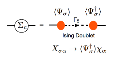
Figure 4: Showing conduction electron self-energy $\Sigma_{c}$. Hybridization with spinorial order parameter $\langle\Psi_{\sigma}\rangle$ permits the development of a $\Gamma_{5}$ Ising resonance inside the conduction sea, represented by the above Feynman diagram.

To encompass the Hubbard operators in a field-theory description, we factorize them as follows

$$X_{\sigma\alpha}=|\Gamma_{7}^{+}\sigma\rangle\langle\Gamma_{5}\alpha|=\hat{\Psi}^{\dagger}_{\sigma}\chi_{\alpha}.$$ (29)

Here $|\Gamma_{5}\alpha\rangle=\chi^{\dagger}_{\alpha}|\Omega\rangle$ is the non-Kramers doublet, represented by the pseudo-fermions $\chi^{\dagger}_{\alpha}$, while $\hat{\Psi}_{\sigma}^{\dagger}$ are slave bosonsColeman83 representing the excited $f^{1}$ doublet $|\Gamma_{7}^{+}\sigma\rangle=\hat{\Psi}^{\dagger}_{\sigma}|\Omega\rangle$. Hastatic order is realized as then condensation of this bosonic spinor

$${\Psi}_{\sigma}^{\dagger}\chi_{\alpha}\rightarrow\langle\hat{\Psi}_{\sigma}\rangle\chi_{\alpha},$$ (30)

generating a hybridization between the conduction electrons and the Ising $5f^{2}$ state while also breaking double time reversal (see Fig. 4). These slave bosons play a dual role in capturing the hybridization while also acting as Schwinger bosons describing a $5f^{1}$ magnetic moment with a reduced amplitude, $2-n_{f}$. The tensor product $Q_{\alpha\beta}\equiv\Psi_{\alpha}\Psi^{\dagger}_{\beta}$ describes the development of composite order between the non-Kramers doublet and the spin density of conduction electrons. Composite order has been considered by several earlier authors in the context of two channel Kondo latticesCox96 ; CATK ; Hoshino11 in which the valence fluctuations have been integrated out. However, by factorizing the composite order in terms of the spinor $\Psi_{\alpha}$, we are able to directly understand the development of coherent Ising quasiparticles and the broken double time-reversal.

There are two general aspects of this condensation that deserve special comment. First, the two-channel Anderson impurity model is known to possess a non-Fermi liquid ground-state with an entanglement entropy of $\frac{1}{2}k_{B}\ln 2$Bolech02 . The development of hastatic order in the lattice liberates this zero-point entropy, accounting naturally for the large entropy of condensation. As a slave boson, $\Psi$ carries both the charge $e$ of the electrons and the local gauge charge $Q_{j}=\Psi^{\dagger}_{j}\Psi_{j}+\chi^{\dagger}_{j}\chi_{j}$ of constrained valence fluctuations, its condensation gives a mass to their relative phase via the Higgs mechanismmarston03 . But as a Schwinger boson, the condensation of $\Psi$ this process breaks the SU (2) spin symmetry. In this way the hastatic boson can be regarded as a magnetic analog of the Higgs boson.

I.5 Structure of the Paper

To recap, here we are arguing that the observation of an anisotropic conduction fluid in URu₂Si₂ indicates the coherent admixture of spin $\frac{1}{2}$ electrons with integer spin doublets, leading us to propose that the order parameter in URu₂Si₂ is spinorial hybridization that breaks both single- and double-time reversal. In conventional heavy fermion materials, hybridization is driven by valence fluctuations between a Kramers doublet and an excited singlet in a single channel. The hybridization carries no quantum numbers and develops as a crossover resulting in heavy mobile electrons. However if the ground-state is a non-Kramers doublet, the Kondo effect occurs via an excited state with an odd number of elections that is a Kramers doublet. The quasiparticle hybridization then carries a global spin quantum number and has two distinct amplitudes that form a spinor defining the hastatic order parameter

$$\Psi=\left(\begin{matrix}\psi_{\uparrow}\cr\psi_{\downarrow}\end{matrix}\right).$$ (31)

The onset of hybridization must break spin rotational invariance in addition to double time-reversal invariance via a phase transition; we note that optical, spectroscopic and tunneling probes in URu₂Si₂ indicate the hybridization occurs abruptly at the hidden order transition in contrast to the crossover behavior observed in other heavy fermion systems.

We now describe the structure of this paper. The microscopic basis of hastatic order is presented using a two-channel Anderson lattice model in section II, along with the mean field solution. In section III, we develop the Landau-Ginzburg theory of hastatic order, including the appearance of pressure induced antiferromagnetism and the nonlinear susceptibility, while in section IV, we derive and discuss a number of experimental consequences of hastatic order, showing the consistency of hastatic order with a number of experiments, including the large entropy of condensation and tetragonal symmetry breaking observed in torque magnetometry, and then making a number of key predictions, including a tiny staggered basal plane moment in the conduction electrons. We end with discussion and future implications in section V.

II Landau theory: Pressure-induced antiferromagnetism

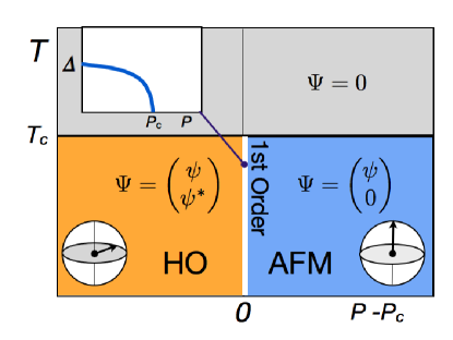
Figure 5: Global phase diagram predicted by Landau theory.

II.1 Thermodynamics

Hastatic order captures the key features of the observed pressure-induced first-order phase transition in URu₂Si₂ between the hidden order and an Ising antiferromagnetic (AFM) phases. The most general Landau functional for the free energy density of a hastatic state with a spinorial order parameter $\Psi$ as a function of pressure and temperature is

$$f[\Psi]=\alpha(T_{c}-T)|\Psi|^{2}+\beta|\Psi|^{4}-\gamma(\Psi^{\dagger}\sigma_{z}\Psi)^{2}$$ (32)

where $\gamma=\delta(P-P_{c})$ is a pressure-tuned anisotropy term and

$$\Psi=r\left(\begin{matrix}\cos(\theta/2)e^{i\phi/2}\cr\sin(\theta/2)e^{-i\phi/2}\end{matrix}\right),$$ (33)

where $\theta$ is the disclination of $\Psi^{\dagger}\vec{\sigma}\Psi$ from the c-axis, and $|\Psi|^{2}=r^{2}$. Experimentally the $T_{AFM}(P)$ line is almost vertical, indicating by the Clausius-Clapeyron relation that the there will be negligible change in entropy between the HO and the AFM states. Indeed these two phases share a number of key features, including common Fermi surface pockets; this has prompted the proposal that they are linked by “adiabatic continuity”, associated by a notational rotation in the space of internal parameters. This is easily accommodated with a spinor order parameter; for the AFM phase ($P>P_{c}$), there is a large staggered Ising f-moment with

$$\Psi_{A}\propto\left(\begin{matrix}1\cr 0\end{matrix}\right),\qquad\Psi_{B}\propto\left(\begin{matrix}0\cr 1\end{matrix}\right)$$ (34)

corresponding to time-reversed spin configurations on alternating layers $A$ and $B$. For the HO state ($P<P_{c}$), the spinor points in the basal plane

$$\Psi_{A}\propto\frac{1}{\sqrt{2}}\left(\begin{matrix}e^{-i\phi/2}\cr e^{i\phi/2}\cr\end{matrix}\right),\qquad\Psi_{B}\propto\frac{1}{\sqrt{2}}\left(\begin{matrix}-e^{-i\phi/2}\cr e^{i\phi/2}\cr\end{matrix}\right)$$ (35)

where $\Psi_{B}=\Theta\Psi_{b}$ and there is no Ising f-moment, consistent with experiment, but Ising fluctuations do exist.

According to the above expression for $\Psi$, $(\Psi^{\dagger}\sigma_{z}\Psi)=r^{2}\cos\theta$ so that the Landau functional can be re expressed as

$$f=-\alpha(T-T_{c})r^{2}+(\beta-\gamma\cos^{2}\theta)r^{4}.$$ (36)

If $P<P_{c}$, then $\gamma<0$ and the minimum of the free energy occurs for $\theta=\pi/2$, corresponding to the hidden order state ordered state. By contrast, if $P>P_{c}$, then $\gamma>0$ and the minimum of the free energy occurs at $\theta=\{0,\pi\}$, corresponding to the antiferromagnet. The “spin flop” in $\theta$ at $P=P_{c}$ corresponds to a first order phase transition between the hidden order and antiferromagnet (See Fig. 5).

II.2 Soft modes and dynamics

The adiabatic continuity between the hastatic and antiferromagnetic phases allows for a simple interpretation of the soft longitudinal spin fluctuations that have been observed to develop in the HO state Broholm91 ; Wiebe07 , and even to go soft, but not critical upon approaching $T_{HO}$Niklowitz11 . These longitudinal modes can be thought of as incipient Goldstone excitations between the two phasesHaule10 . Specifically, in the HO state, rotations of the hastatic spinor out of the basal plane will lead to a gapped Ising collective mode like the one observed. Within our Landau theory, we can study the evolution of this mode with pressure.

In order to study the soft modes of the hastatic order, we need to generalize the Landau theory to a time-dependent Landau Ginzburg theory for the action, with action $S=\int Ldtd^{3}x$, where the Lagrangian

$$-L[\Psi]=f[\Psi]+\rho\left(|\nabla\Psi|^{2}-c^{-2}|\dot{\Psi}|^{2}\right),$$

and $\rho$ is the stiffness. Expanding $\Psi$ around its equilibrium value $\Psi_{0}$, we take $\phi=0$ for convenience and write

$$\Psi(x,t)=\Psi_{0}e^{i\delta\theta(x)\sigma_{y}/2}=(1+i/2\sum_{q}\delta\theta(q)e^{i\vec{q}\cdot\vec{x}-\omega t}\sigma_{y})\Psi_{0}.$$ (37)

This gives rise to a change in $\Psi^{\dagger}\vec{\sigma}\Psi=\hat{x}|\Psi_{0}|^{2}+\delta\theta(x)\hat{z}|\Psi_{0}|^{2}$ corresponding to a fluctuation in the longitudinal magnetization. This rotation in $\Psi$ does not affect the first two isotropic terms in $f[\Psi]$. The variation in the action is then given by

$$\delta S=\rho|\Psi_{0}|^{2}\sum_{q}|\theta(q)|^{2}\left(\vec{q}^{\ 2}-\frac{\omega^{2}}{c^{2}}+\frac{2\delta}{\rho}(P_{c}-P)|\Psi_{0}|^{2}\right)$$ (38)

The dispersion is therefore

$$\omega^{2}=(cq)^{2}+\Delta^{2}$$ (39)

where

$$\Delta^{2}=\frac{2\delta(P_{c}-P)}{\rho}|\Psi_{0}|^{2},$$ (40)

so that even though the phase transition at $P=P_{c}$ is first order, the gap for longitudinal spin fluctuations is

$$\Delta\propto|\Psi_{0}|\sqrt{P_{c}-P}.$$

Since $dP_{c}/dT_{c}$ is finite, close to the transition, $\sqrt{P_{c}-P}\approx\sqrt{dP_{c}/dT_{c}(T-T_{c})}$, and $\Delta\propto\sqrt{T-T_{c}}$. Inelastic neutron scattering experiments can measure this gap a function of temperature at a fixed pressure where there is a finite temperature first order transition. The iron-doped compound, URu_2-xFe_xSi₂ can provide an attractive alternative to hydrostatic pressure, as iron doping acts as uniform chemical pressure and tunes the hidden order state into the antiferromagnetbutch .

However, higher order terms, like $\lambda(\Psi^{\dagger}\sigma_{z}\Psi)^{2}|\Psi|^{2}$ are also allowed by symmetry, and will introduce a weak discontinuity of order $|\Psi_{0}|^{4}$,

$$\Delta^{2}=\frac{2\delta(P_{c}-P)}{\rho}|\Psi_{0}|^{2}+\frac{2\lambda}{\rho}|\Psi_{0}|^{4}+O(|\Psi_{0}|^{6}).$$ (41)

So there will likely always be a discontinuity in the longitudinal spin fluctuation mode at the first order phase transition, although it will be of a lower order ($|\Psi_{0}|^{4}$) than a generic first order transition ($|\Psi_{0}^{2}|$).

III Microscopic Model: Two-Channel Anderson Lattice

Hastatic order emerges as a spinorial hybridization between a non-Kramers doublet ground state and a Kramers doublet excited state. In our picture of URu₂Si₂, a lattice of $5f^{2}$ ($J=4$) U⁴⁺ ions provide the non-Kramers doublet ($\Gamma_{5}$), which are then surrounded by a sea of conduction electrons that facilitate valence fluctuations between the $5f^{2}$ non-Kramers doublet and a $5f^{1}$ or $5f^{3}$ excited Kramers doublet. The two-channel Anderson lattice model has three components:

$$H=H_{c}+\sum_{j}\left[H_{VF}(j)+H_{a}(j)\right],$$ (42)

a conduction electron term, $H_{c}$, a valence fluctuation term capturing how the conduction electrons hop on and off the U site, $H_{VF}$ and an atomic Hamiltonian capturing the different energy levels of the U ion, $H_{a}$.

III.1 The Valence Fluctuation Hamiltonian

III.1.1 The $5f^{1}$ model

The $5f^{2}$ $\Gamma_{5}$ non-Kramers doublet is given by

$$|5f^{2}:\Gamma_{5}\pm\rangle=a|\pm 3\rangle+b|\mp 1\rangle,$$ (43)

and all energies are measured relative to the energy of this isolated doublet. In principle, valence fluctuations may either occur to $5f^{1}$ ($J=5/2$) or to $5f^{3}$ ($J=9/2$), and in fact the lowest lying excited state is likely to be the $5f^{3}$ state. However, for technical simplicity, we take the lowest lying valence fluctuation excitation to be the $5f^{1}$ $\Gamma_{7}^{+}$ excited state,

$$|5f^{2}:\Gamma_{5}\pm\rangle\rightleftharpoons|5f^{1}:\Gamma_{7}^{+}\pm\rangle+e^{-}$$ (44)

where

$$|5f^{1}:\Gamma_{7}^{+}\pm\rangle=\eta|\pm 5/2\rangle+\delta|\mp 3/2\rangle$$ (45)

is the excited Kramers doublet. The following section will show how particle-hole symmetry can be used to formulate the equivalent model with fluctuations into a $5f^{3}$ Kramers doublet.

To evaluate the matrix elements for valence fluctuations we need to express the $5f^{2}$ state in terms of one-particle states. The $\Gamma_{5}$ state can be rewritten as a product of the one particle $J=5/2$ f-orbitals, $|5/2,m\rangle\equiv f^{\dagger}_{m}|\Omega\rangle$, using the Clebsch Gordan decomposition

$$|\mp 1\rangle = \left(\sqrt{\frac{5}{7}}f^{\dagger}_{\pm 1/2}f^{\dagger}_{\mp 3/2}+\sqrt{\frac{2}{7}}f^{\dagger}_{\pm 3/2}f^{\dagger}_{\mp 5/2}\right)|\Omega\rangle,$$ (46)

$$|\pm 3\rangle = f^{\dagger}_{\pm 5/2}f^{\dagger}_{\mp 1/2}|\Omega\rangle.$$ (47)

Next we decompose the one-particle f-states in terms of the one-particle crystal field eigenstates, $|\Gamma\pm\rangle\equiv f^{\dagger}_{\Gamma,\pm}|\Omega\rangle$; writing $f^{\dagger}_{m}=f^{\dagger}_{\Gamma\beta}\langle\Gamma\beta|m\rangle$, or more explicitly,

$$f^{\dagger}_{\pm 1/2} = f^{\dagger}_{\Gamma_{6}\pm}$$ (48)

$$f^{\dagger}_{\mp 3/2} = \delta f^{\dagger}_{\Gamma_{7}^{+}\pm}-\eta f^{\dagger}_{\Gamma_{7}^{-}\pm}$$ (49)

$$f^{\dagger}_{\pm 5/2} = \eta f^{\dagger}_{\Gamma_{7}^{+}\pm}+\delta f^{\dagger}_{\Gamma_{7}^{-}\pm}$$ (50)

the non-Kramer’s doublet can be written in the form

$$|\Gamma_{5}+\rangle = ({p}f^{\dagger}_{\Gamma_{7}^{-}\downarrow}f^{\dagger}_{\Gamma_{7}^{+}\downarrow}+{q}f^{\dagger}_{\Gamma_{6}\uparrow}f^{\dagger}_{\Gamma_{7}^{+}\uparrow}+{s}f^{\dagger}_{\Gamma_{6}\uparrow}f^{\dagger}_{\Gamma_{7}^{-}\uparrow})|\Omega\rangle$$ (51)

$$|\Gamma_{5}-\rangle = ({p}f^{\dagger}_{\Gamma_{7}^{-}\uparrow}f^{\dagger}_{\Gamma_{7}^{+}\uparrow}+{q}f^{\dagger}_{\Gamma_{6}\downarrow}f^{\dagger}_{\Gamma_{7}^{+}\downarrow}+{s}f^{\dagger}_{\Gamma_{6}\downarrow}f^{\dagger}_{\Gamma_{7}^{-}\downarrow})|\Omega\rangle,$$ (52)

where ${p}=b\sqrt{\frac{2}{7}}$, ${q}=b\delta\sqrt{\frac{5}{7}}-a\eta$, ${s}=-b\delta\sqrt{\frac{5}{7}}-a\eta$. Valence fluctuations from the ground state (5f² $\Gamma_{5}$) to the excited state (5f¹ $\Gamma_{7}^{+}$) are described by a a one-particle Anderson model with an on-site hybridization term

$$H_{VF}(j)=\sum_{\Gamma=\Gamma_{6},\Gamma_{7}^{\pm};\sigma}\left[v_{\Gamma}{c}^{\dagger}_{\Gamma\sigma}(j)f_{\Gamma\sigma}(j)+{\rm H.c}\right],$$ (54)

where the $v_{\Gamma}$ are the hybridization matrix elements in the three orthogonal crystal field channels and ${c}^{\dagger}_{\Gamma\sigma}(j)$ creates a conduction electron in a Wannier state with symmetry $\Gamma\sigma$ on site $j$.

Now we need to project this Hamiltonian down into the reduced subspace of the ground-state $|5f^{2}:\Gamma_{5}\alpha\rangle$ and $|5f^{1}:\Gamma_{7}^{-}\sigma\rangle$ excited state doublets, replacing

$$f_{\Gamma\sigma}(j)\rightarrow\sum_{\sigma^{\prime},\alpha=\pm}|\Gamma_{7}^{+}\sigma^{\prime}\rangle\Biggl{(}\langle\Gamma_{7}^{+}\sigma^{\prime}|f_{\Gamma\sigma}(j)|\Gamma_{5}\alpha\rangle\Biggr{)}\langle\Gamma_{5}\alpha|$$ (55)

in (54). Using (51), the only non-vanishing matrix elements between the $5f^{2}$ and $5f^{1}$ states are

$$\langle\Gamma_{7}^{+}\mp|f_{\Gamma_{7}^{-}\mp}|\Gamma_{5}\pm\rangle = p,$$ (56)

$$\langle\Gamma_{7}^{+}\pm|f_{\Gamma_{6}\pm}|\pm\rangle = q.$$ (57)

Matrix elements for the $\Gamma_{7}^{+}$ channel identically vanish $\langle\Gamma_{7}^{+}\sigma|f_{\Gamma_{7}^{+}\pm}|\sigma^{\prime}\rangle=0$, so the third term in (51) does not contribute to the projected Hamiltonian. The final projected model is then written

$$H=\sum_{{\bf{k}}\sigma}\epsilon_{{\bf{k}}}c^{\dagger}_{{\bf{k}}\sigma}c_{{\bf{k}}\sigma}+\sum_{j}\left[H_{VF}(j)+H_{a}(j)\right]$$ (58)

where $c^{\dagger}_{{\bf{k}}\sigma}$ creates a conduction electron of momentum ${\bf{k}}$ spin $\sigma$, with energy $\epsilon_{{\bf{k}}}$, and

$$H_{VF}(j) = V_{6}{c}_{\Gamma_{6}\pm}^{\dagger}(j)|\Gamma_{7}^{+}\pm\rangle\langle\Gamma_{5}\pm|$$ (59)

$$+ V_{7}{c}_{\Gamma^{-}_{7}\mp}^{\dagger}(j)|\Gamma_{7}^{+}\mp\rangle\langle\Gamma_{5}\pm|+\mathrm{H.c.}$$ (60)

describes the valence fluctuations between the $\Gamma_{5}$ doublet and the excited $\Gamma_{7}^{+}$ Kramers doublet. Here $V_{6}=v_{\Gamma_{6}}q$ and $V_{7}=v_{\Gamma_{7}^{-}}p$ while

$$H_{a}(j)=\Delta E\sum_{\pm}|\Gamma_{7}\pm\rangle\langle\Gamma_{7}\pm|$$ (61)

is the atomic Hamiltonian for the excited $5f^{1}:\Gamma_{7}^{+}$ Kramers doublet. Notice that, as we have projected out most of the possible U states, we are working in terms of the Hubbard operators, $|\Gamma_{5}\pm\rangle$ and $|\Gamma_{7}\pm\rangle$ to describe the allowed U states.

To further develop the valence fluctuation term, we need to determine the form factors relating the conduction electron Wannier states in terms of Bloch waves,

$${c}^{\dagger}_{\Gamma\alpha}=\sum_{\bf{k}}c^{\dagger}_{{\bf{k}}\beta}\left[\Phi_{\Gamma{\bf{k}}}\right]_{\beta\alpha}\mathrm{e}^{-i{\bf{k}}\cdot{\bf{R}}_{j}}.$$ (62)

For a single site interacting with a plane wave, these are given by $\left[\Phi_{\Gamma{\bf{k}}}\right]_{\alpha\beta}=y^{\Gamma}_{\alpha\beta}({\bf{k}})$, where

$$y^{\Gamma}_{\alpha\beta}({\bf{k}}) = \sum_{m=-5/2}^{5/2}Y_{3m-\frac{\alpha}{2}}(\hat{\bf{k}})\langle 3m-\frac{\alpha}{2},\frac{1}{2}\frac{\alpha}{2}|5/2m\rangle{\langle m|\Gamma,\ \beta\rangle}$$ (63)

$$= \alpha\sum_{m=-5/2}^{5/2}\sqrt{\frac{1}{2}-\frac{m\alpha}{7}}\ Y_{3m-\frac{\alpha}{2}}(\hat{\bf{k}}){\langle m|\Gamma\beta\rangle}.$$ (64)

where $\alpha,\beta\in\pm$. However, in URu₂Si₂, the uranium atoms are located on a body centered tetragonal(bct) lattice at relative locations, ${\bf{R}}_{NN}=(\pm a/2,\pm a/2,\pm c/2)$, and the correct form factor must respective the lattice symmetries. Our model treats the conduction band as a single band of s-electrons located at the U sites. Moreover, we assume that the f-electrons hybridize via electron states at the nearby silicon atoms located at ${\bf{a}}_{NN}=(\pm a/2,\pm a/2,\pm z)$ where $z=.371c$ is the height of the silicon atom above the U atomOppeneer10 . The form-factor is then

$$\left[\Phi_{\Gamma{\bf{k}}}\right]_{\alpha\beta}=\sum_{\{{\bf{R}}_{NN},{\bf{a}}_{NN}\}}e^{-i{\bf{k}}\cdot({\bf R}_{NN}-{\bf a}_{NN})}\times e^{-i{\bf{k}}\cdot{\bf a}_{NN}}y^{\Gamma}_{\alpha\beta}({\bf{a}}_{NN})=\sum_{\{{\bf{R}}_{NN},{\bf{a}}_{NN}\}}e^{-i{\bf{k}}\cdot{\bf R}_{NN}}y^{\Gamma}_{\alpha\beta}({\bf{a}}_{NN}).$$ (66)

Here, the term $e^{-i{\bf{k}}\cdot{\bf a}_{NN}}y^{\Gamma}_{\alpha\beta}({\bf{a}}_{NN})$ is the amplitude to hybridize with the silicon site at site ${\bf a}_{NN}$, while the prefactor $e^{-i{\bf{k}}\cdot({\bf R}_{NN}-{\bf a}_{NN})}$ is the additional phase factor for hopping from the silicon site ${\bf a}_{NN}$ to the U atom, ${\bf R}_{NN}$ directly above it. This form of the hybridization can also be derived using Slater-Kosterslater methods, under the assumption that the important part of the hybridization potential is symmetric about the axis between the U and Si atom. Notice that this function has the following properties: $\left[\Phi_{\Gamma{\bf{k}}+{\bf G}}\right]_{\alpha\beta}=\left[\Phi_{\Gamma{\bf{k}}}\right]_{\alpha\beta}$ and $\left[\Phi_{\Gamma{\bf{k}}+{\bf{Q}}}\right]_{\alpha\beta}=-\left[\Phi_{\Gamma{\bf{k}}}\right]_{\alpha\beta}$. We should note that this model of the hybridization is overly simplified, in that the U most likely hybridizes with the d-electrons sitting on the Ru site. Such a d-f hybridization can be treated in a similar fashion, and is the subject of future work.

III.1.2 The $5f^{3}$ case

For simplicity we have discussed the two channel Anderson model involving fluctuations from a $5f^{2}$ $\Gamma_{5}$ ground state to $5f^{1}$ ($J=5/2$). However, the more realistic case involves fluctuations to $5f^{3}$, whose low energy states have $J=9/2$, and are split into five Kramers doublets by the tetragonal crystal field,

$$|\Gamma_{6}^{\lambda}\pm\rangle = c^{\lambda}|\pm 9/2\rangle+d^{\lambda}|\pm 1/2\rangle+e^{\lambda}|\mp 7/2\rangle,$$ (67)

$$|\Gamma_{7}^{1}\pm\rangle = a|\pm 5/2\rangle+b|\mp 3/2\rangle$$ (68)

$$|\Gamma_{7}^{2}\pm\rangle = -b|\pm 5/2\rangle+a|\mp 3/2\rangle,$$ (69)

where $\lambda\in(1,2,3)$ labels the three $\Gamma_{6}$ Kramer’s doublets. There are two generic situations: either a $\Gamma_{7}$ doublet is lowest in energy, and the valence fluctuations are then determined by the overlap,

$$|\Gamma_{7}\pm\rangle=\alpha\psi^{\dagger}_{6\mp}|\Gamma_{5}\pm\rangle+\beta\psi^{\dagger}_{7\mp}|\Gamma_{5}\mp\rangle,$$ (70)

or alternatively, a $\Gamma_{6}$ doublet is lowest in energy, with the relevant overlap,

$$|\Gamma_{6}\pm\rangle=\alpha\psi^{\dagger}_{7\mp}|\Gamma_{5}\pm\rangle+\beta\psi^{\dagger}_{6\mp}|\Gamma_{5}\mp\rangle,$$ (71)

where the form-factors are as above. In both cases fluctuations will involve conduction electrons in both $\Gamma_{6}$ and $\Gamma_{7}$ symmetries. When the lowest excited state is a $\Gamma_{7}$, the valence fluctuation Hamiltonian is given by,

$$H_{VF3}(j) = V_{6}(\psi_{j\Gamma_{6}\mp}^{\dagger}|\Gamma_{5}\pm\rangle\langle\Gamma_{7}\pm|+{\rm H.c})$$ (72)

$$+ V_{7}(\psi_{j\Gamma_{7}\mp}^{\dagger}|\Gamma_{5}\mp\rangle\langle\Gamma_{7}\pm|+\mathrm{H.c.}).$$ (73)

The only difference between the $5f^{3}$ and the $5f^{1}$ model is that the excited state requires adding a particle, so the valence fluctuation term here is the particle-hole conjugate of the $5f^{1}$ case.

III.2 Slave particle treatment

Hubbard operators cannot be directly treated with quantum field theory techniques since they do not satisfy Wick’s theorem. We follow the standard approach and introduce a slave particle factorization of the Hubbard operators that permits a field theoretic treatment,

$$|\Gamma_{7}^{+}\sigma\rangle\langle\Gamma_{5}\alpha|=\hat{\Psi}^{\dagger}_{\sigma}\chi_{\alpha}.$$ (74)

where

$$|\Gamma_{5}\alpha\rangle=\chi^{\dagger}_{\alpha}|\Omega\rangle$$ (75)

is the non-Kramers doublet, represented by the pseudo-fermion $\chi^{\dagger}_{\alpha}$, while $\hat{\Psi}_{\sigma}^{\dagger}$ is a slave bosonColeman83 representing the excited $f^{1}$ doublet

$$|\Gamma_{7}^{+}\sigma\rangle=\hat{\Psi}^{\dagger}_{\sigma}|\Omega\rangle$$ (76)

that carries a positive charge and a spin quantum number. Condensation of the spin-$\frac{1}{2}$ boson then gives rise to the hastatic order parameter

$${\bf{\Psi}}=\begin{pmatrix}\langle\hat{\Psi}_{\uparrow}\rangle\cr\langle\hat{\Psi}_{\downarrow}\rangle\end{pmatrix}.$$ (77)

This condensation process that we may now replace the Hubbard operator $\hat{X}_{\sigma\alpha}$ by a single bound-state fermion

$${\Psi}_{\sigma}^{\dagger}\chi_{\alpha}\rightarrow\langle\hat{\Psi}_{\sigma}\rangle\chi_{\alpha}.$$ (78)

We may interpret this replacement as a kind of multi-particle contraction of the many body Hubbard operator into a single fermionic bound-state. Once this bound-state forms, a symmetry-breaking hybridization develops between the conduction electrons and the Ising $5f^{2}$ state.

The dual Schwinger/slave character of the boson $\hat{\Psi}^{\dagger}_{\sigma}$ representing the occupation of $5f^{1}$ means when this field condenses, it not only breaks the local $U(1)$ gauge symmetry, but also the global $SU(2)$ spin symmetry. However, it breaks the $U(1)$ gauge symmetry as a slave boson, which have been well studied in the context of heavy fermions. The $U(1)$ phase of the local gauge symmetry is subject to the Anderson-Higgs mechanism, in which the difference between the electromagnetic gauge field and the internal $U(1)$ gauge field acquires a massmarston03 . It is this process that gives the $\chi$ fermions a physical charge. The combination of the global and local symmetry breaking processes means that the hastatic order parameter can be thought of as a magnetic Higgs boson.

With this slave particle factorization, we can reformulate

$$\sum_{j}H_{a}(j)\rightarrow\Delta E\sum_{j,\sigma=\pm}\Psi^{\dagger}_{\sigma}(j)\Psi_{\sigma}(j).$$ (79)

The valence fluctuation term at each site takes the form

$$H_{VF}(j) = V_{6}{c}_{\Gamma_{6}\pm}^{\dagger}(j)\Psi_{\pm}^{\dagger}(j)\chi_{\pm}(j)+V_{7}{c}_{\Gamma^{-}_{7}\mp}^{\dagger}(j)\Psi^{\dagger}_{\mp}(j)\chi_{\pm}(j)$$ (80)

$$+ \mathrm{H.c.}.$$ (81)

We now rewrite this expression in terms of Bloch waves by absorbing the momentum dependent Wannier form-factors into the spin-dependent hybridization matrix, introducing the operator

$$\hat{\mathcal{V}}({\bf{k}},j)=V_{6}\Phi_{\Gamma_{6}}B^{\dagger}_{j}+V_{7}\Phi_{\Gamma_{7}^{-}}\hat{B}^{\dagger}_{j}\sigma_{1}.$$ (82)

where the matrix

$$\hat{B}^{\dagger}_{j}=\left(\begin{matrix}\hat{\Psi}^{\dagger}_{j\uparrow}&0\cr 0&\hat{\Psi}^{\dagger}_{j\downarrow}\end{matrix}\right)$$ (83)

contains the hastatic boson. The valence fluctuation term then becomes

$$H_{VF}(j)=\sum_{\bf{k}}c^{\dagger}_{{\bf{k}}\sigma}\hat{\mathcal{V}}_{\sigma\alpha}({\bf{k}},j)\chi_{\alpha}(j)\mathrm{e}^{-i{\bf{k}}\cdot{\bf{R}}_{j}}+\mathrm{H.c.}$$ (84)

Putting these results all together, our model for URu₂Si₂ is given by

$$H = \sum_{{\bf{k}}\sigma}\epsilon_{{\bf{k}}}c^{\dagger}_{{\bf{k}}\sigma}c_{{\bf{k}}\sigma}+\sum_{{\bf{k}}}\left[c^{\dagger}_{{\bf{k}}\sigma}\left(V_{6}\Phi_{\Gamma_{6}}B^{\dagger}_{j}+V_{7}\Phi_{\Gamma_{7}^{-}}\hat{B}^{\dagger}_{j}\sigma_{1}\right)\chi_{\alpha}(j)e^{-i{\bf{k}}\cdot{\bf{R}}_{j}}+{\rm H.c.}\right]+\Delta E\sum_{j,\sigma=\pm}\Psi^{\dagger}_{\sigma}(j)\Psi_{\sigma}(j)$$ (85)

$$+ \sum_{j}\lambda_{j}\left(\sum_{\sigma}\Psi^{\dagger}_{\sigma}(j)\Psi_{\sigma}(j)+\sum_{\alpha}\chi^{\dagger}_{\alpha}(j)\chi_{\alpha}(j)-1\right).$$ (86)

The respective terms in this Hamiltonian describe the conduction electrons, the hybridization between the excited Kramers and ground-state non-Kramers doublets, the energy $\Delta E$ of the excited Kramers doublets. The second line of the Hamiltonian describes the constraint $n_{\Psi}(j)+n_{\chi}(j)=1$ associated with the slave boson representation. Finally notice that if we compare (85) with the parent Anderson model (54), the original f-annihilation operators in the $\Gamma_{6}$ and $\Gamma_{7^{-}}$ channel have been replaced as follows:

$$f_{\Gamma_{6}\alpha}(j)\rightarrow(B^{\dagger}_{j}\chi_{j})_{\alpha},\qquad f_{\Gamma_{7}\alpha}(j)\rightarrow(B^{\dagger}_{j}\sigma_{1}\chi_{j})_{\alpha}.$$ (87)

So while $\chi_{\pm}$ is a slave particle representing the non-Kramers doublet, these operators represent composite fermions in the two hybridization channels, with all the quantum numbers of an electron.

III.3 Mean Field Theory for Hastatic Order

III.3.1 Mean Field Hamiltonian: a spinorial order parameter

The central element of the mean field theory is the hastatic order parameter, described by a two-component spinor. We consider the following configurations

$${\bf\Psi}\equiv\langle\hat{\Psi}_{\sigma}\rangle=\begin{pmatrix}e^{-i({\bf{Q}}\cdot{\bf{R}}_{j}+\phi)/2}\cr e^{i({\bf{Q}}\cdot{\bf{R}}_{j}+\phi)/2}\end{pmatrix}.$$ (88)

where ${\bf{Q}}=(0,0,\frac{2\pi}{c})$, corresponding to a hybridization that is staggered between planes, with a spinorial order parameter that points in the Basal plane, rotated through an angle $\phi$ around the c-axis. Eventually, we shall choose $\phi=\pi/4$ to provide a 45⁰ rotation of the scattering t-matrix relative to the x-axis, an orientation that provides consistency with the measured $\chi_{xy}$ anomaly in the bulk susceptibilityOkazaki11 .

Next, in (82) we make the substitution

$$\langle\hat{\cal V}({\bf{k}},j)\rangle=V_{6}\Phi_{\Gamma_{6}}\langle\hat{B}^{\dagger}_{j}\rangle+V_{7}\Phi_{\Gamma_{7}^{-}}\langle\hat{B}^{\dagger}_{j}\rangle\sigma_{1}.$$ (89)

It is convenient to write $\langle B^{\dagger}_{j}\rangle$ in the form

$$\langle\hat{B}^{\dagger}_{j}\rangle=|\Psi|U_{j},$$ (90)

where

$$U_{j}=\left(\begin{matrix}e^{i({\bf{Q}}\cdot{\bf{R}}_{j}+\phi)/2}&\cr&e^{-i({\bf{Q}}\cdot{\bf{R}}_{j}+\phi)/2}\end{matrix}\right)$$ (91)

is a diagonal unitary matrix.

The gauge symmetry of the slave particle representation allows us to redefine the f-electrons, $\tilde{\chi}_{j}=U_{j}\chi_{j}$ to absorb the spatial dependence of $\langle\hat{B}_{j}^{\dagger}\rangle$ into the redefined f-electrons(87), so that

$$\hat{B}^{\dagger}_{j}\chi_{j}=|\Psi|\tilde{\chi}_{j}$$ (92)

and

$$\hat{B}^{\dagger}_{j}\sigma_{1}\chi_{j}=|\Psi|(U_{j}\sigma_{1}U^{\dagger}_{j})\tilde{\chi}_{j}=|\Psi|(\hat{\bf{n}}\cdot\vec{\sigma})e^{i{\bf{Q}}\cdot{\bf{R}}_{j}}\tilde{\chi}_{j},$$ (93)

where $\hat{\bf{n}}=\frac{1}{\sqrt{2}}(\hat{\bf{x}}+\hat{\bf{y}})$ is the unit-vector representing the orientation of the hastatic spinor. The commensurate nature of the wavevector is important, as here we have used the fact that $e^{i{\bf{Q}}\cdot{\bf{R}}_{j}}\equiv(-1)^{z_{j}/c}$ is real. In this gauge, the $\Gamma_{6}$ hybridization is uniform while the $\Gamma_{7}^{-}$ hybridization is staggered. In preparation for our transition to momentum space, we write

$${\cal V}_{6}({\bf{k}})=|\Psi|V_{6}\Phi^{6}({\bf{k}}),$$ (94)

and

$${\cal V}_{7}({\bf{k}})=|\Psi|V_{7}\Phi^{7}({\bf{k}})(\hat{\bf{n}}\cdot\vec{\sigma}),$$ (95)

where we introduce the short-hand $\Phi^{6}({\bf{k}})\equiv\Phi_{\Gamma_{6}}({\bf{k}})$ and $\Phi^{7}({\bf{k}})\equiv\Phi_{\Gamma_{7}^{-}}({\bf{k}})$. Notice that ${\cal V}_{6}({\bf{k}}+{\bf{Q}})=-{\cal V}_{6}({\bf{k}})$ and ${\cal V}_{7}({\bf{k}}+{\bf{Q}})=-{\cal V}_{7}({\bf{k}})$ both change sign when shifted by ${\bf{Q}}$. In the slave formulation, the atomic Hamiltonian is $H_{a}(j)=\Delta E\sum_{\sigma}\Psi^{\dagger}_{j\sigma}\Psi_{j\sigma}=\Delta E|\Psi|^{2}$.

While we treat the hybridization between the conduction electrons and the f-moments very carefully, we take a simple model of the conduction electron hopping, treating them as s-wave electrons located at the U sites, hopping on a bct lattice with dispersion

$$\epsilon_{\bf{k}}=-8t\cos\frac{k_{x}a}{2}\cos\frac{k_{y}a}{2}\cos\frac{k_{z}c}{2}-\mu.$$ (96)

We do, however, want to capture the essential characteristics of the URu₂Si₂ bandstructure - namely nesting between an electron Fermi surface about the zone center and a hole Fermi surface at ${\bf{Q}}$Oppeneer10 . In order to favor a staggered hybridization, and to match up with ARPES experiments suggesting a heavy f-bandSantander09 , we take the hole Fermi surface to be generated from a weakly dispersing $\chi$ band. This f-electron hopping will be naturally generated by hybridization fluctuations above $T_{HO}$, effectively where $\langle\hat{B}^{\dagger}\hat{B}\rangle\neq 0$ while $\langle\hat{B}\rangle=0$. A large $N$ expansion of this problem would capture these fluctuation effects, but is overly complicated for this problem so we put this dispersion in by hand, $\epsilon_{f{\bf{k}}}=-8t_{f}\cos\frac{k_{x}a}{2}\cos\frac{k_{y}a}{2}\cos\frac{k_{z}c}{2}$. So to summarize, our mean-field Hamiltonian is,

$$H = \sum_{\bf{k}}\epsilon_{\bf{k}}c^{\dagger}_{{\bf{k}}\sigma}c_{{\bf{k}}\sigma}+\sum_{\bf{k}}(\epsilon_{f{\bf{k}}}+\lambda)\chi^{\dagger}_{{\bf{k}}\eta}\chi_{{\bf{k}}\eta}+{\cal N}_{s}\left[(\Delta E+\lambda)|\Psi|^{2}-1\right]$$ (97)

$$+ \sum_{{\bf{k}}}\left[c^{\dagger}_{{\bf{k}}\sigma}\left({\cal V}_{6\sigma\alpha}({\bf{k}})\chi_{{\bf{k}}\alpha}+{\cal V}_{7\sigma\alpha}({\bf{k}})\chi_{{\bf{k}}+{\bf{Q}}\alpha}\right)+{\rm H.c}\right].$$ (98)

where we have dropped the tilde’s on the $\chi_{{\bf{k}}}$ and ${\cal N}_{s}$ is the number of sites in the lattice. We rewrite this Hamiltonian in matrix form

$$H=\sum_{\bf{k}}\left(c^{\dagger}_{\bf{k}},c^{\dagger}_{{\bf{k}}+{\bf{Q}}},\chi^{\dagger}_{\bf{k}},\chi^{\dagger}_{{\bf{k}}+{\bf{Q}}}\right)\overbrace{\left(\begin{matrix}\epsilon_{\bf{k}}&0&\mathcal{V}_{6}({\bf{k}})&\mathcal{V}_{7}({\bf{k}})\cr 0&\epsilon_{{\bf{k}}+{\bf{Q}}}&-\mathcal{V}_{7}({\bf{k}})&-\mathcal{V}_{6}({\bf{k}})\cr\mathcal{V}_{6}^{\dagger}({\bf{k}})&-\mathcal{V}_{7}^{\dagger}({\bf{k}})&\lambda_{\bf{k}}&0\cr\mathcal{V}_{7}^{\dagger}({\bf{k}})&-\mathcal{V}_{6}^{\dagger}({\bf{k}})&0&\lambda_{{\bf{k}}+{\bf{Q}}}\end{matrix}\right)}^{{\cal H}_{\alpha\beta}({\bf{k}})}\left(\begin{array}[]{c}c_{\bf{k}}\\ c_{{\bf{k}}+{\bf{Q}}}\\ \chi_{{\bf{k}}}\\ \chi_{{\bf{k}}+{\bf{Q}}}\end{array}\right)+{\cal N}_{s}\left[(\Delta E+\lambda)|\Psi|^{2}-\lambda\right].$$ (103)

where we have suppressed spin indices, made the assumption that the Lagrange multiplier $\lambda_{j}=\lambda$ is uniform, equivalent to enforcing the constraint on average, introduced $\lambda_{\bf{k}}=\lambda+\epsilon_{f{\bf{k}}}$, and used the simplification that ${\bf{Q}}$ is half a reciprocal lattice vector, making $\mathcal{V}({\bf{k}}+{\bf{Q}})=-\mathcal{V}({\bf{k}})$, as shown above. When we diagonalize this Hamiltonian, we obtain a a set of four doubly degenerate bands, $E_{{\bf{k}}\eta}$. These eigenvalues can be obtained analytically in the special case where the band-structure has particle-hole symmetry, but more generally they must be obtained numerically.

The corresponding mean field free energy is then

$$F[b,\lambda] = -\frac{\beta^{-1}}{2}\sum_{{\bf{k}},\eta}\log\left[1+\mathrm{e}^{-\beta E_{{\bf{k}}\eta}}\right]$$ (105)

$$+\mathcal{N}_{s}\left[2(\Delta E+\lambda)|\Psi|^{2}-\lambda\right],$$

where $\beta=(k_{B}T)^{-1}$. In the work presented here, the mean field parameters, $|\Psi|$ and $\lambda$ are obtained by numerically finding a stationary point that minimizes $F$ with respect to $|\Psi|$ and maximizes it with respect to $\lambda$.

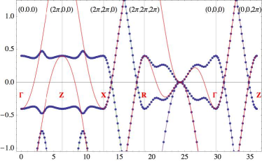
Figure 6: Band structure of the hastatic order is shown in solid blue, while the bare conduction (red) and f (green) bands are dashed. The parameters used for this calculation are given in section III.3.2.

III.3.2 Mean field parameters

In order to plot the band structure and calculate semi-realistic experimental quantities, we have chosen the following parameters: the internal hastatic angle, $\phi=\pi/4$ is chosen to reproduce $\chi_{xy}\neq 0$ type tetragonal symmetry breaking; t = 12.5 meV is taken to match the magnitude of $\chi_{xy}$ from the torque magnetometry dataOkazaki11 ; $\mu/t=-.075$ gives the slight particle-hole asymmetry essential to reproduce the flattening of $\chi_{xy}$ at low temperatures, and has also been adjusted so that $\mu+\lambda=0$ at $T=0$ for consistency with the dI/dV calculations (see later section); $t_{f}/t=-.025$ gives a weak f-electron dispersion; the crystal field angle $\xi=.05$ is taken to be small, as it is in CeRu₂Si₂Haen92 and NdRu₂Si₂; $V_{6}/V_{7}=1$ is arbitrary; and finally $V^{2}/\Delta E=2t$ is chosen to give $2|\Psi|^{2}\approx 15\%$ mixed valency. The actual degree of mixed valency in URu₂Si₂ is unknown, with 15% being an upper estimate. The band-structure corresponding to these parameters is shown in Fig. 6.

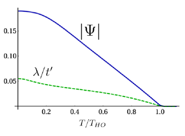
Figure 7: Mean field parameters $|\Psi|$ and $\lambda$ as a function of temperature. The parameters used for this calculation are given in section III.3.2.

A plot of $|\Psi|$ and $\lambda$ as a function of temperature is shown in Figure 7 B, for these parameters. $|\Psi|$ controls the amplitude of the hybridization gap opening at $T_{HO}$, while $\lambda$ controls the location of the hybridization gap center in energy. We plot the band structure, both above $T_{HO}$ (dashed lines) and at zero temperature (solid lines) in the hastatic phase, and the integrated density of states, to show how hastatic order opens up a gap above $E_{F}$.

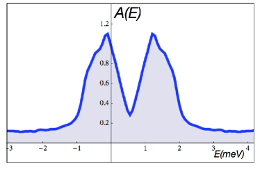
Figure 8: Density of states in with hastatic order, for the region close to the Fermi energy containing the hybridization gap. The parameters used for this calculation are given in section III.3.2.

The total density of states is given by

$$A(\omega) = \sum_{{\bf{k}}\eta}\delta(\omega-E_{{\bf{k}}\eta})$$ (106)

$$= \frac{1}{\pi}{\rm Im}\int\frac{d^{3}k}{(2\pi)^{3}}\sum_{\eta}\frac{1}{\omega-E_{{\bf{k}}\eta}-i\delta}$$ (107)

where the integral is over the Brillouin zone. The results of a numerical calculation of the above density of states are shown in Fig. 8 C. The calculation was carried out with a discrete summation over momenta, dividing the Brillouin zone into $40^{3}$ points and using a small value of $\delta$ to broaden the delta-function into a Lorentzian.

III.4 Conduction and f-electron Green’s functions

In order to calculate various moments and susceptibilities, we will require the full conduction electron Green’s function, which can be found from the Hamiltonian by integrating out the f-electrons,

$$\left[\mathcal{G}^{c}({\bf{k}},i\omega)\right]^{-1}=\left(\begin{matrix}i\omega_{n}-\epsilon_{\bf{k}}&0\cr 0&i\omega_{n}-\epsilon_{{\bf{k}}+{\bf{Q}}}\end{matrix}\right)-\mathcal{V}_{{\bf{k}}}\left(\begin{matrix}i\omega_{n}-\lambda_{\bf{k}}&0\cr 0&i\omega_{n}-\lambda_{{\bf{k}}+{\bf{Q}}}\end{matrix}\right)^{-1}\mathcal{V}^{\dagger}_{\bf{k}},$$ (108)

where

$$\mathcal{V}_{\bf{k}}=\left(\begin{matrix}\mathcal{V}_{6{\bf{k}}}&\mathcal{V}_{7{\bf{k}}}\cr-\mathcal{V}_{7{\bf{k}}}&-\mathcal{V}_{6{\bf{k}}}\end{matrix}\right).$$ (109)

Using isospin, $\vec{\tau}$ to represent ${\bf{k}},{\bf{k}}+{\bf{Q}}$ space, we split the conduction electron energy, $\epsilon_{\bf{k}}$ into $\epsilon_{0{\bf{k}}}=\frac{1}{2}\left(\epsilon_{{\bf{k}}}+\epsilon_{{\bf{k}}+{\bf{Q}}}\right)$, $\epsilon_{1{\bf{k}}}=\frac{1}{2}\left(\epsilon_{{\bf{k}}}-\epsilon_{{\bf{k}}+{\bf{Q}}}\right)$ into the particle-hole symmetric and antisymmetric parts (and similarly with $\lambda_{0{\bf{k}}},\lambda_{1{\bf{k}}}$). So now we can write the conduction electron Green’s function as:

$$\left[\mathcal{G}^{c}({\bf{k}},i\omega)\right]^{-1}=(i\omega_{n}-\epsilon_{0{\bf{k}}})-\epsilon_{1{\bf{k}}}\tau_{3}-\Sigma_{c}({\bf{k}},i\omega_{n}),$$ (110)

where

$$\Sigma_{c}({\bf{k}},i\omega_{n})=\mathcal{V}\frac{i\omega_{n}-\lambda_{0{\bf{k}}}+\lambda_{1{\bf{k}}}\tau_{3}}{(i\omega_{n}-\lambda_{0{\bf{k}}})^{2}-\lambda_{1{\bf{k}}}^{2}}\mathcal{V}^{\dagger}$$ (111)

is the self-energy generated by resonant Kondo scattering off the hastatic order. The scattering terms in this quantity are determined by two matrices, a diagonal, symmetry-preserving matrix $\mathcal{V}_{{\bf{k}}}\mathcal{{V}}^{\dagger}_{{\bf{k}}}$ and a symmetry-breaking $\mathcal{V}_{{\bf{k}}}\tau_{3}\mathcal{{V}}^{\dagger}_{{\bf{k}}}$. We decompose these matrices into their channel and spin components as follows:

$$\mathcal{V}_{{\bf{k}}}\mathcal{{V}}^{\dagger}_{{\bf{k}}} = V^{2}_{{\bf{k}}c+}+(\vec{\Delta}_{{\bf{k}}c+}\cdot\vec{\sigma})\tau_{1},$$ (112)

$$\mathcal{V}_{{\bf{k}}}\tau_{3}\mathcal{{V}}^{\dagger}_{{\bf{k}}} = V^{2}_{{\bf{k}}c-}+\Delta_{{\bf{k}}c-}\tau_{2},$$ (113)

where the only non-vanishing components are:

$$V_{{\bf{k}}c+}^{2} = \frac{1}{4}{\hbox{Tr}}\left[\mathcal{V}_{\bf{k}}\mathcal{V}_{\bf{k}}^{\dagger}\right]=\frac{1}{2}{\hbox{Tr}}\left[\mathcal{V}_{6{\bf{k}}}\mathcal{V}_{6{\bf{k}}}^{\dagger}+\mathcal{V}_{7{\bf{k}}}\mathcal{V}_{7{\bf{k}}}^{\dagger}\right]$$ (114)

$$V_{{\bf{k}}c-}^{2} = \frac{1}{4}{\hbox{Tr}}\left[\mathcal{V}_{\bf{k}}\tau_{3}\mathcal{V}_{\bf{k}}^{\dagger}\tau_{3}\right]=\frac{1}{2}{\hbox{Tr}}\left[\mathcal{V}_{6{\bf{k}}}\mathcal{V}_{6{\bf{k}}}^{\dagger}-\mathcal{V}_{7{\bf{k}}}\mathcal{V}_{7{\bf{k}}}^{\dagger}\right]$$ (115)

$$\overrightarrow{\Delta}_{{\bf{k}}c+} = \frac{1}{4}{\hbox{Tr}}\left[\mathcal{V}_{\bf{k}}\mathcal{V}_{\bf{k}}^{\dagger}\tau_{1}\vec{\sigma}\right]=-\frac{1}{2}{\hbox{Tr}}\left[\left(\mathcal{V}_{6{\bf{k}}}\mathcal{V}_{7{\bf{k}}}^{\dagger}+\mathcal{V}_{7{\bf{k}}}\mathcal{V}_{6{\bf{k}}}^{\dagger}\right)\vec{\sigma}\right]$$ (116)

$$\Delta_{{\bf{k}}c-} = \frac{1}{4}{\hbox{Tr}}\left[\mathcal{V}_{\bf{k}}\tau_{3}\mathcal{V}_{\bf{k}}^{\dagger}\tau_{2}\right]=\frac{i}{2}{\hbox{Tr}}\left[\mathcal{V}_{6{\bf{k}}}\mathcal{V}_{7{\bf{k}}}^{\dagger}-\mathcal{V}_{7{\bf{k}}}\mathcal{V}_{6{\bf{k}}}^{\dagger}\right].$$ (117)

We note that the non-zero form factor $\Delta_{{\bf{k}}c-}$ which involves a product of hybridization in different channels ${\cal V}_{6{\bf{k}}}$ and ${\cal V}_{7{\bf{k}}}$ has a d-wave form factor, reflecting the fact that electron scattering off hastatic order parameter breaks tetragonal lattice symmetry. The related form factor that describes the c-electron moments, $\overrightarrow{\Delta}_{{\bf{k}}c-}$ is a vector in spin space which is even parity in momentum space. Under time-reversal, this component changes sign and therefore breaks time-reversal symmetry.

The Green’s function can now be written in the form $\left[\mathcal{G}\right]^{-1}=A\tau_{0}+B\tau_{3}+\vec{C}\cdot\vec{\sigma}\tau_{1}+D\tau_{2}$. The eigenvalues are found by taking $\det\left[\mathcal{G}^{c}({\bf{k}},\omega)\right]^{-1}=0$, leading to an eighth order polynomial that cannot be generically solved analytically, except in the special case of particle-hole symmetry. The four (doubly degenerate) eigenvalues are $E_{{\bf{k}}\eta}$ and are found numerically on a grid of ${\bf{k}}$ points. Due to the structure of the Green’s function, we can write,

$$\mathcal{G}^{c}(i\omega_{n},{\bf{k}}) = \frac{1}{\prod_{\eta}(i\omega_{n}-E_{{\bf{k}}\eta})}\left(A_{c{\bf{k}}}(i\omega_{n})\tau_{0}-B_{c{\bf{k}}}(i\omega_{n})\tau_{3}-\vec{C}_{c{\bf{k}}}(i\omega_{n})\cdot\vec{\sigma}\tau_{1}-D_{c{\bf{k}}}\tau_{2}\right),$$ (118)

$$A_{c{\bf{k}}}(i\omega_{n}) = (i\omega_{n}-\epsilon_{0{\bf{k}}})\left[(i\omega_{n}-\lambda_{0{\bf{k}}})^{2}-\lambda_{1{\bf{k}}}^{2}\right]-(i\omega_{n}-\lambda_{0{\bf{k}}})V_{{\bf{k}}c+}^{2}$$ (119)

$$B_{c{\bf{k}}}(i\omega_{n}) = -\epsilon_{1{\bf{k}}}\left[(i\omega_{n}-\lambda_{0{\bf{k}}})^{2}-\lambda_{1{\bf{k}}}^{2}\right]-\lambda_{1{\bf{k}}}V_{{\bf{k}}-}^{2}$$ (120)

$$\vec{C}_{c{\bf{k}}}(i\omega_{n}) = -(i\omega_{n}-\lambda_{0{\bf{k}}})\overrightarrow{\Delta}_{{\bf{k}}c+}$$ (121)

$$D_{c{\bf{k}}}(i\omega_{n}) = -\lambda_{1{\bf{k}}}\Delta_{{\bf{k}}c-}.$$ (122)

Once $E_{{\bf{k}}\eta}$ is obtained numerically, this structure makes calculations with the conduction electron Green’s function fairly straightforward, as we shall illustrate in sections IV.2 and V.3. The f-electron Green’s function can be obtained by integrating out the conduction electrons, and is quite similar

$$\left[\mathcal{G}^{f}({\bf{k}},i\omega)\right]^{-1}=(i\omega_{n}-\lambda_{0{\bf{k}}})-\lambda_{1{\bf{k}}}\tau_{3}-\mathcal{V}^{\dagger}\frac{i\omega_{n}-\epsilon_{0{\bf{k}}}+\epsilon_{1{\bf{k}}}\tau_{3}}{(i\omega_{n}-\epsilon_{0{\bf{k}}})^{2}-\epsilon_{1{\bf{k}}}^{2}}\mathcal{V}.$$ (123)

The main difference is that the hybridization terms will be of the form ${\hbox{Tr}}\mathcal{V}_{\bf{k}}^{\dagger}({\bf 1},\tau_{3})\mathcal{V}_{\bf{k}}\tau_{a}\sigma_{b}$, as given below. We note that $V_{{\bf{k}}f+}^{2}=V_{{\bf{k}}c+}^{2}={\hbox{Tr}}\mathcal{V}_{\bf{k}}^{\dagger}\mathcal{V}_{\bf{k}}$, and $\Delta_{{\bf{k}}f-}=\Delta_{{\bf{k}}c-}$ are the same for the c- and f-electrons. There is only one new, non-zero term,

$$\overrightarrow{\Delta}_{{\bf{k}}f+} = \frac{1}{4}{\hbox{Tr}}\mathcal{V}^{\dagger}_{\bf{k}}\mathcal{V}_{\bf{k}}\tau_{1}\vec{\sigma}=-\frac{1}{2}{\hbox{Tr}}\left[\left(\mathcal{V}^{\dagger}_{6{\bf{k}}}\mathcal{V}_{7{\bf{k}}}+\mathcal{V}_{7{\bf{k}}}^{\dagger}\mathcal{V}_{6{\bf{k}}}\right)\vec{\sigma}\right].$$ (124)

that breaks time-reversal symmetry and generally has a d-wave symmetry.

The f-electron Green’s function is then,

$$\mathcal{G}^{f}(i\omega_{n},{\bf{k}}) = \frac{1}{\prod_{\eta}(i\omega_{n}-E_{{\bf{k}}\eta})}\left(A_{f{\bf{k}}}(i\omega_{n})\tau_{0}-B_{f{\bf{k}}}(i\omega_{n})\tau_{3}-\vec{C}_{f{\bf{k}}}(i\omega_{n})\cdot\vec{\sigma}\tau_{1}-D_{f{\bf{k}}}\tau_{2}\right),$$ (125)

$$A_{f{\bf{k}}}(i\omega_{n}) = (i\omega_{n}-\lambda_{0{\bf{k}}})\left[(i\omega_{n}-\epsilon_{0{\bf{k}}})^{2}-\epsilon_{1{\bf{k}}}^{2}\right]-(i\omega_{n}-\epsilon_{0{\bf{k}}})V_{{\bf{k}}c+}^{2}$$ (126)

$$B_{f{\bf{k}}}(i\omega_{n}) = -\lambda_{1{\bf{k}}}\left[(i\omega_{n}-\epsilon_{0{\bf{k}}})^{2}-\epsilon_{1{\bf{k}}}^{2}\right]-\epsilon_{1{\bf{k}}}V_{{\bf{k}}c-}^{2}$$ (127)

$$\vec{C_{f{\bf{k}}}}(i\omega_{n}) = -(i\omega_{n}-\epsilon_{0{\bf{k}}})\overrightarrow{\Delta}_{{\bf{k}}f+}$$ (128)

$$D_{f{\bf{k}}} = -\epsilon_{1{\bf{k}}}\Delta_{{\bf{k}}c-}.$$ (129)

We will examine the ${\bf{k}}$-space structure of these terms, and the related moments, in section V.3.

III.5 Particle-Hole Symmetric Case

For the special case of a particle-hole symmetric dispersion, where $(\epsilon_{{\bf{k}}+{\bf{Q}}}+\mu)=-(\epsilon_{\bf{k}}+\mu)$ and $\epsilon_{f{\bf{k}}+{\bf{Q}}}=-\epsilon_{f{\bf{k}}}$, we can solve the Hamiltonian (103) exactly provided $\lambda+\mu=0$, so that $\epsilon_{0{\bf{k}}}=\lambda_{0{\bf{k}}}=\lambda=-\mu$ are both dispersionless. In fact, the simple c- and f-dispersions we have chosen already satisfy particle-hole symmetry, so the special case $\lambda=-\mu$ provides a limit where we can obtain analytic results. In this case, $\epsilon_{0{\bf{k}}}=\lambda_{0{\bf{k}}}=\lambda$, and the the determinant of the Green’s function can be calculated from (110). We wish to evaluate the determinant ${\rm det}\left[{\omega-H({\bf{k}})}\right]$, where $H({\bf{k}})$ is the matrix Hamiltonian given in (103). By integrating out the f-electrons we can factorize the determinant into a product of the full-conduction electron determinant and the bare f-electron determinant as follows obtain

$${\rm det}\left[{\omega-H({\bf{k}})}\right] = {\rm det}\left[{-{\cal G}^{c}({\bf{k}},\omega)^{-1}}\right]{\rm det}\left[{\omega-\lambda_{0{\bf{k}}}-\lambda_{1{\bf{k}}}\tau_{3}}\right]$$ (130)

$$= {\rm det}\left[{-{\cal G}^{c}({\bf{k}},\omega)^{-1}}\right]((\omega-\lambda_{0{\bf{k}}})^{2}-\lambda_{1{\bf{k}}}^{2})^{2}$$ (131)

where the overall square in the second factor results from the two-fold spin degeneracy and

$${\rm det}[-{\cal G}^{c}({\bf{k}},\omega)^{-1}]={\rm det}\left[{(\omega-\epsilon_{0{\bf{k}}})-\epsilon_{1{\bf{k}}}\tau_{3}-{\cal V}_{{\bf{k}}}\frac{\omega-\lambda_{0{\bf{k}}}+\lambda_{1{\bf{k}}}\tau_{3}}{(\omega-\lambda_{0{\bf{k}}})^{2}-\lambda_{1{\bf{k}}}^{2}}{\cal V}^{\dagger}_{{\bf{k}}}}\right]$$ (132)

We now impose particle-hole symmetry, setting $\lambda_{0{\bf{k}}}=\lambda=\epsilon_{0{\bf{k}}}=-\mu$. For convenience, we redefine $z=\omega-\lambda$. Then

$${\rm det}\left[{\omega-H({\bf{k}})}\right] = {\rm det}[-{\cal G}^{c}({\bf{k}},\omega)^{-1}](z^{2}-\lambda_{1k}^{2})^{2}$$ (133)

$$= {\rm det}\left[{z-\epsilon_{1{\bf{k}}}\tau_{3}-{\cal V}_{{\bf{k}}}\frac{z+\lambda_{1{\bf{k}}}\tau_{3}}{z^{2}-\lambda_{1{\bf{k}}}^{2}}{\cal V}^{\dagger}_{{\bf{k}}}}\right](z^{2}-\lambda_{1k}^{2})^{2}$$ (134)

$$= {\cal D}^{2}(z)/(z^{2}-\lambda_{1{\bf{k}}}^{2})^{2}$$ (135)

where we have multiplied all four rows of the determinant by $z^{2}-\lambda_{1{\bf{k}}}^{2}$ and have defined

$${\cal D}^{2}(z)={\rm det}\left[{(z-\epsilon_{{\bf{k}}}\tau_{3})(z^{2}-\lambda_{1{\bf{k}}}^{2})-{\cal V}_{{\bf{k}}}({z+\lambda_{1{\bf{k}}}\tau_{3}}){\cal V}^{\dagger}_{{\bf{k}}}}\right].$$ (136)

Note that since this is a four dimensional determinant, ${\cal D}^{2}(z)$ is a twelfth order polynomial. Now by employing the shorthand $V_{+}^{2}\equiv V_{{\bf{k}}c+}^{2}$, $V_{-}^{2}\equiv V_{{\bf{k}}c-}^{2}$, $\vec{\Delta}_{+}\equiv\vec{\Delta}_{{\bf{k}}c+}$ and $\Delta_{-}\equiv\Delta_{{\bf{k}}c-}$, and substituting $\mathcal{V}_{{\bf{k}}}\mathcal{{V}}^{\dagger}_{{\bf{k}}}=V^{2}_{+}+(\vec{\Delta}_{+}\cdot\vec{\sigma})\tau_{1}$ and $\mathcal{V}_{{\bf{k}}}\tau_{3}\mathcal{{V}}^{\dagger}_{{\bf{k}}}=V^{2}_{-}+\Delta_{-}\tau_{2}$ from (114), we obtain

$${\cal D}^{2}(z)={\rm det}\left[{z(z^{2}-\lambda_{1{\bf{k}}}^{2}-V_{+}^{2})-(z^{2}-\lambda_{1{\bf{k}}}^{2})\epsilon_{1{\bf{k}}}\tau_{3}-z\vec{\Delta}_{+}\cdot\vec{\sigma}\tau_{1}-\lambda V_{-}^{2}\tau_{3}-\Delta_{-}\lambda_{1{\bf{k}}}\tau_{2}}\right].$$ (137)

If we normalize $\vec{\Delta}_{+}=\Delta_{+}\hat{n}$, then the triplet of matrices $(\gamma_{1},\gamma_{2},\gamma_{3})\equiv((\hat{n}\cdot\vec{\sigma})\tau_{1},\tau_{2},\tau_{3})$ forms a triplet of anticommuting Dirac matrices, ($\{\gamma_{i},\gamma_{j}\}=2\delta_{ij}$), which satisfy the charge conjugation symmetry $U\gamma_{i}U^{\dagger}=-\gamma_{i}^{T}$, ($i\in[1,3]$), where $U=\sigma_{2}\tau_{2}$. Since the determinant is unchanged under this transformation, it is unchanged under a reversal $\gamma_{i}\rightarrow-\gamma_{i}$. If we take the product of the $\gamma$-reversed determinant with itself, the resulting “squared” determinant is then diagonal, giving

$${\cal D}^{4}(z)={\rm Det}\biggl{[}\biggl{(}z^{2}(z^{2}-\lambda_{1{\bf{k}}}^{2}-V_{+}^{2})^{2}-(z^{2}-\lambda_{1{\bf{k}}}^{2})^{2}\epsilon_{1{\bf{k}}}^{2}-z^{2}\Delta_{+}^{2}-\lambda_{1{\bf{k}}}^{2}V_{-}^{4}-\Delta_{-}^{2}\lambda_{1{\bf{k}}}^{2}\biggr{)}\mathds{1}_{4}\biggr{]}.$$ (138)

And since the argument of the determinant is a diagonal four-dimensional matrix,

$${\cal D}(z)=z^{2}(z^{2}-\lambda_{1{\bf{k}}}^{2}-V_{+}^{2})^{2}-(z^{2}-\lambda_{1{\bf{k}}}^{2})^{2}\epsilon_{1{\bf{k}}}^{2}-z^{2}\Delta_{+}^{2}-\lambda_{1{\bf{k}}}^{2}V_{-}^{4}-\Delta_{-}^{2}\lambda_{1{\bf{k}}}^{2},$$ (139)

Now there can be no poles in ${\rm det}[\omega-H({\bf{k}})]$ at $z=\lambda_{1{\bf{k}}}$, so ${\cal D}(z)$ must have zeros at $z=\pm\lambda_{1{\bf{k}}}$ to cancel the denominator in ${\rm det}\left[{\omega-H({\bf{k}})}\right]={\cal D}^{2}(z)/(z^{2}-\lambda_{1{\bf{k}}}^{2})^{2}$. We can factorize the determinant as follows:

$${\cal D}(z)=(z^{2}-\lambda_{1{\bf{k}}}^{2})\biggl{(}z^{2}(z^{2}-\lambda_{1{\bf{k}}}^{2}-2V_{+}^{2})-\epsilon_{1{\bf{k}}}^{2}(z^{2}-\lambda_{1{\bf{k}}}^{2})-2\epsilon_{1{\bf{k}}}\lambda_{1{\bf{k}}}V_{-}^{2}\biggr{)}+z^{2}(V_{+}^{4}-\Delta_{+}^{2})-\lambda_{1{\bf{k}}}^{2}(V_{-}^{4}+\Delta_{-}^{2}).$$ (140)

Now since $D(z=\lambda_{1{\bf{k}}})=0$ is a zero, it follows that

$$V_{+}^{4}-V_{-}^{4}=\Delta_{+}^{2}+\Delta_{-}^{2},$$ (141)

which also follows somewhat nonintuitively from the form-factor definitions, allowing us to rewrite

$${\cal D}(z) = (z^{2}-\lambda_{1{\bf{k}}}^{2})\biggl{(}z^{2}(z^{2}-\lambda_{1{\bf{k}}}^{2}-2V_{+}^{2}-\epsilon_{1{\bf{k}}}^{2})+(\epsilon_{1{\bf{k}}}\lambda_{1{\bf{k}}}-V_{-}^{2})^{2}+\Delta_{-}^{2}\biggl{)}$$ (142)

$$= (z^{2}-\lambda_{1{\bf{k}}}^{2})\biggl{(}z^{4}-2z^{2}\left(V_{+}^{2}+\frac{1}{2}(\epsilon_{1{\bf{k}}}^{2}+\lambda_{1{\bf{k}}}^{2})\right)+(\epsilon_{1{\bf{k}}}\lambda_{1{\bf{k}}}-V_{-}^{2})^{2}+\Delta_{-}^{2}\biggl{)}.$$ (143)

Therefore, by (133)

$${\rm det}\left[{\omega-H({\bf{k}})}\right]=\left[(\omega-\lambda)^{4}-2\alpha_{\bf{k}}(\omega-\lambda)^{2}+\gamma_{\bf{k}}^{2}\right]^{2}$$ (144)

where

$$\alpha_{\bf{k}} = V_{{\bf{k}}c+}^{2}+\frac{1}{2}\left(\epsilon_{1{\bf{k}}}^{2}+\lambda_{1{\bf{k}}}^{2}\right)$$ (145)

$$\gamma_{\bf{k}}^{2} = \left(\epsilon_{1{\bf{k}}}\lambda_{1{\bf{k}}}-V_{{\bf{k}}c-}^{2}\right)^{2}+\Delta_{{\bf{k}}c-}^{2}.$$ (146)

The square in the determinant reflects a two-fold Kramers degeneracy associated with the invariance of the physics under a combined translation and time reversal. The energy eigenstates are then determined by the condition

$$(\omega-\lambda)^{4}-2\alpha_{\bf{k}}(\omega-\lambda)^{2}+\gamma_{\bf{k}}^{2}=0,$$ (147)

The four bands are then given by,

$$E_{{\bf{k}}\eta}=\lambda\pm\sqrt{\alpha_{{\bf{k}}}\pm\sqrt{\alpha_{\bf{k}}^{2}-\gamma_{\bf{k}}^{2}}},$$ (148)

where $\eta=1-4$ labels the $++$, $+-$, $-+$ and $--$ bands.

III.6 Hybridization gaps

As hastatic order is, at its heart, a spinorial hybridization, the nature of the resulting hybridization gaps is essential to understanding the order. In fact, there are generically two types of gaps: those that break one or more symmetries: translation, spin rotation, crystal or time-reversal symmetries, and those that break no symmetries. In our mean-field picture, the intra-channel gaps, $V_{{\bf{k}}c\pm}^{2}$ break no symmetries and are proportional to the amplitude of the hastatic spinor, $\langle\Psi^{\dagger}\Psi\rangle$, while the inter-channel gap, $\Delta_{{\bf{k}}c-}$ breaks all of the above symmetries and is proportional to $\langle\Psi^{\dagger}\vec{\sigma}\Psi\rangle$. The role of these form-factors as hybridization gaps is especially clear in the particle-hole symmetric case, (148), where their relative roles may be distinguished. While in the mean-field theory, all hybridization gaps will develop at $T_{HO}$, we believe that hastatic order will melt via phase fluctuations, destroying the coherence of the symmetry breaking gap, but keeping the symmetry preserving gaps. The existence of two types of hybridization gaps that turn on at different temperatures can reconcile the number of experiments that find hybridization gaps turning on either at $T_{HO}$Schmidt10 ; Aynajian10 or around the coherence temperature $T^{*}\sim 50-70$KPark11 ; Haraldsen11 . In addition, these hybridization gaps will connect different parts of the Fermi surface as the intra-channel gaps carry ${\bf Q}=0$, while the inter-channel gap connects the folded bands.

The symmetry-breaking hybridization gap $\Delta_{{\bf{k}}c-}$, shown in Fig. 9 (a) has an approximate four-fold “d-wave” symmetry about a nematic axis $\hat{n}$ lying in the basal plane (Fig. 9 (b,c)). While only the square of the inter-channel gap appears in equation (148), it plays the same role as the superconducting gap in composite pairingnphysus , and the nodal structure has corresponds to a changing phase of the hybridization between c- and f-electrons around the Brillouin zone. The modulus of the gap, $|\Delta_{{\bf{k}}c-}|$ carries a nematicity, whereby the moments of the gap function squared averaged over the Fermi surface,

$$\left\langle\Delta_{{\bf{k}}c-}^{2}\hat{k}_{\alpha}\hat{k}_{\beta}\right\rangle_{FS}\propto\hat{n}_{\alpha}\hat{n}_{\beta}$$ (149)

define a secondary nematic director $\hat{n}=(n_{x},n_{y})$ of magnitude

$$\hat{n}_{x,y}\propto\Psi^{\dagger}{\sigma}_{x,y}\Psi$$ (150)

proportional to the square of the hastatic order parameter. The orientation of the nematicity is set by $\phi$, here chosen to be $\phi=\pi/4$. The tetragonal symmetry breaking can be tuned by changing the crystal field parameter, $\xi$, but cannot be eliminated. However, as the tetragonal symmetry breaking is d-wave in nature, it can not couple linearly to strain and therefore will not lead to a first order structural transition.

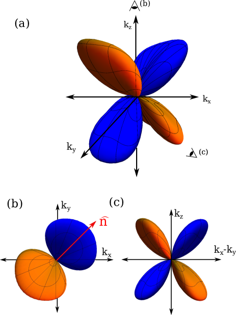
Figure 9: (a) Three dimensional plot showing the symmetry breaking component of the hybridization gap, $\Delta_{{\bf{k}}c-}$ for the chosen crystal field parameters, $\xi=.05$ and for $\phi=\pi/4$. Orange and blue represent positive and negative values of the gap. The gap lobes are oriented in the plane along the nematic director $\hat{n}$ shown in the figure. (b) Top view showing the nematic character of the gap function, aligned along the nematic director $\hat{n}$ (c) Side view along the axis of the nematic director $\hat{n}$ showing its nodal d-wave structure.

IV Comparison to Experiment: Postdictions

IV.1 g-factor Anisotropy

The Zeeman energy is determined by the Hamiltonian

$$-\vec{B}\cdot\vec{M}=-\sum_{{\bf{k}}\in\frac{1}{2}BZ}\psi^{\dagger}_{{\bf{k}}}{\vec{\cal M}}\psi_{{\bf{k}}}\cdot\vec{B}$$ (151)

where $\psi_{{\bf{k}}}=(c_{{\bf{k}}},c_{{\bf{k}}+{\bf{Q}}},\chi_{{\bf{k}}},\chi_{{\bf{k}}+{\bf{Q}}})^{T}$ and

$$\vec{{\cal M}}=\frac{1}{2}\left(\begin{matrix}2\mu_{B}\vec{\sigma}&0&0&0\cr 0&2\mu_{B}\vec{\sigma}&0&0\cr 0&0&{g_{f}}\mu_{B}{\sigma^{z}}&0\cr 0&0&0&{g_{f}}\mu_{B}{\sigma^{z}}\end{matrix}\right),$$ (152)

where $g_{f}$ is the effective g-factor of the Ising Kramers doublet. In a field, the doubly-degenerate energies, $|{\bf{k}}\eta\sigma\rangle$ ($\sigma=\pm 1$) are split apart so that $\Delta E_{{\bf{k}}\eta}=|E_{{\bf{k}}\eta\uparrow}-E_{{\bf{k}}\eta\downarrow}|=g_{{\bf{k}}\eta}(\theta)B$, so the g-factor is given by $g_{{\bf{k}}\eta}(\theta)=\left|\frac{d\Delta E_{{\bf{k}}\eta}}{dB}\right|_{B\rightarrow 0}$. Now we are interested in the Fermi surface average of the g-factor, given by

$$g(\theta)=\frac{\sum_{{\bf{k}}\eta}g_{{\bf{k}}\eta}(\theta)\delta(E_{{\bf{k}}\eta})}{\sum_{{\bf{k}}\eta}\delta(E_{{\bf{k}}\eta})}$$

These quantities were calculated numerically, on a $40^{3}$ grid, using $g_{f}=2.9$ for the effective g-factor of the local non-Kramers doublet. The resulting g-factor in the $z-$ direction is reduced to $g_{eff}(\theta=0)=2.6$ because of the admixture with conduction electrons. The delta-functions were treated as narrow Lorentzians $\delta(E)=\frac{1}{\pi}Im(E-i\eta)^{-1}$, where $\eta$ is a small positive number. The g-factors at each point in momentum space were computed by introducing a small field $\delta B$ into the Hamiltonian, with the approximation $g_{{\bf{k}}\eta}(\theta)=|E_{{\bf{k}}\uparrow}-E_{{\bf{k}}\downarrow}|/\delta B$.

IV.2 Anisotropic Linear Susceptibility

The uniform basal plane conduction electron magnetic susceptibility acquires a tetragonal symmetry breaking component in the hastatic phase, given by

$$\chi^{xy}=-(g\mu_{B})^{2}T\sum_{i\omega_{n}}\sum_{{\bf{k}}}{\hbox{Tr}}\left[\sigma^{x}\mathcal{G}^{c}({\bf{k}},{\bf{k}}+{\bf{Q}},i\omega_{n})\sigma^{y}\mathcal{G}^{c}({\bf{k}}+{\bf{Q}},{\bf{k}},i\omega_{n})\right].$$ (153)

Expanding this in terms of the conduction electron Green’s function, we obtain

$$\chi^{xy} = -(g\mu_{B})^{2}T\sum_{i\omega_{n}}\sum_{{\bf{k}}}{\hbox{Tr}}\left[\sigma_{x}\mathcal{G}^{c}({\bf{k}},i\omega_{n})\sigma_{y}\mathcal{G}^{c}({\bf{k}},i\omega_{n})\right]$$ (154)

$$= -(g\mu_{B})^{2}\sum_{{\bf{k}}\eta}\left[\frac{2(E_{{\bf{k}}\eta}-\lambda_{0{\bf{k}}})f(E_{{\bf{k}}\eta})+(E_{{\bf{k}}\eta}-\lambda_{0{\bf{k}}})^{2}f^{\prime}(E_{{\bf{k}}\eta})}{\prod_{\eta^{\prime}\neq\eta}(E_{{\bf{k}}\eta}-E_{{\bf{k}}\eta^{\prime}})^{2}}\right.$$ (156)

$$\left.-\sum_{\eta^{\prime}\neq\eta}\frac{2(E_{{\bf{k}}\eta}-\lambda_{0{\bf{k}}})^{2}f(E_{{\bf{k}}\eta})}{{(E_{{\bf{k}}\eta}-E_{{\bf{k}}\eta^{\prime}})}\prod_{\eta^{\prime\prime}\neq\eta}(E_{{\bf{k}}\eta}-E_{{\bf{k}}\eta^{\prime\prime}})^{2}}\right]\Delta^{x}_{{\bf{k}}+}\Delta^{y}_{{\bf{k}}+}$$

Note that above integral may be positive or negative. The functions $f$ and $f^{\prime}$ are the Fermi function, $f(x)=\left(\mathrm{e}^{-x/T}+1\right)^{-1}$ and it’s derivative, $f^{\prime}(x)=df(x)/dx$, respectively. The exact nature of the tetragonal symmetry breaking is determined by the angle of the hastatic spinor, $\phi$; when $\phi=\pi/4$, $\chi_{xx}=\chi_{yy}$, but $\chi_{xy}\neq 0$, but changing $\phi$ can rotate the direction of the tetragonal symmetry breaking.

In our current mean-field approach, all Kondo behavior develops at the hidden order transition, which would lead to an entropy of $R\log 2$ at $T_{HO}$. Incorporating Gaussian fluctuations should suppress the hidden order phase transition, $T_{HO}$, while allowing many of the signatures of heavy fermion physics, including the heavy mass and a partial quenching of the spin entropy to develop at a higher crossover scale, $T_{K}$. The two-channel Kondo impurity has a zero-point entropy of $\frac{1}{2}R\log 2$Destri84 ; Tsvelik85 ; EmeryKivelson92 , which should be incorporated into the hastatic phase. There is considerable uncertainty in the entropy associated with the development of hidden order, $S(T_{HO})$, due to difficulties subtracting the phonon and other non-electronic contributions, leading to estimates ranging from $.15R\log 2$Jaime02 to $.3R\log 2$Palstra85 . If we take a conservative estimate of $S(T_{HO})=.2R\log 2$, and the normal state $\gamma=180{\rm mJ/molK^{2}}$Palstra85 , $S(T_{K})=.2R\log 2+\int_{T_{HO}}^{T_{K}}\gamma dT=\frac{1}{2}R\log 2$ yields $T_{K}=27$K, much lower than the coherence temperature seen in the resistivity.

V Comparison to Experiment: Predictions

V.1 Resonant Nematicity in Scanning Probes

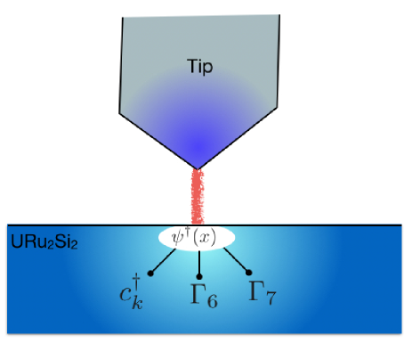
Figure 10: Schematic illustrating the tunneling and co-tunneling into three channels: a conduction, a $\Gamma_{6}$ and a $\Gamma_{6}$ f-electron channel.

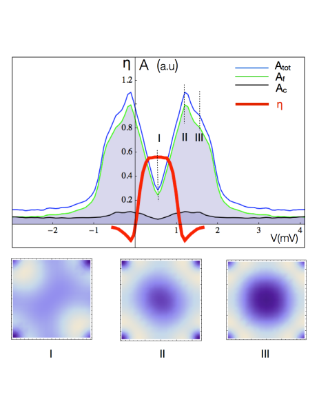
Figure 11: Upper panel: showing the total density of states, decomposed according to f, conduction and total spectral weight. These curves were calculated for a particle-hole symmetric dispersion, setting $\lambda=-\mu$ as described in III C2 and IIIE. The red curve shows energy dependent nematicity. Small panels below show the density of states at three different energies, showing the energy dependence of the nematicity. Reprinted from hastatic .

To calculate the tunneling density of states, we assume that the differential conductance is proportional to the local Green’s function on the surface of the material

$$\frac{dI}{dV}({\bf{x}})\propto A({\bf{x}},eV)$$ (157)

where

$$A({\bf{x}},\omega) = \frac{1}{\pi}{\rm Im}G_{\sigma\sigma}({\bf{x}},\omega-i\delta)$$ (158)

$$= \sum_{\sigma}\int_{-\infty}^{\infty}dt\langle\{\psi_{\sigma}({\bf{x}},t),\psi_{\sigma}^{\dagger}({\bf{x}},0)\}\rangle e^{i\omega t}$$ (159)

is the imaginary part of the local electronic Green’s function.

To calculate this quantity, we decompose the local electron field in terms of the low energy fermion modes of the system. Typically, in a Kondo system, there are two channels - a conduction channel, and a f-electron channel into which the electron may tunnel maltseva09 . However, in URu₂Si₂ the presence of a non-Kramer’s doublet now involves two f-tunneling channels - the $\Gamma_{6}$ and $\Gamma_{7^{-}}$ channel, and tunneling through these three channels can mutually interfere (see Fig. 10). We therefore decompose the electron field $\psi_{\sigma}({\bf{x}})$ in terms of a conduction and two f-electron channels, writing,

$$\psi_{\sigma}({\bf{x}})=\sum_{j}\left(\phi_{c}(|{\bf{x}}-{\bf{R}}_{j}|),\phi^{6}_{\sigma\alpha}({\bf{x}}-{\bf{R}}_{j}),\phi^{7}_{\sigma\alpha}({\bf{x}}-{\bf{R}}_{j})\right)\cdot\begin{pmatrix}c_{j\sigma}\cr f_{j\Gamma_{6}\alpha}\cr f_{j\Gamma_{7}\alpha}\cr\end{pmatrix}$$ (160)

where $\phi_{c}(|{\bf{x}}-{\bf{R}}_{j}|)$ is the wavefunction of the conduction electron centered at site j, while

$$\phi^{6}_{\sigma\alpha}(|{\bf{x}}-{\bf{R}}_{j}|) = \phi^{6}(|{\bf{x}}-{\bf{R}}_{j}|){\cal Y}^{6}_{\sigma\alpha}({\bf{x}}-{\bf{R}}_{j})$$ (161)

$$\phi^{7}_{\sigma\alpha}(|{\bf{x}}-{\bf{R}}_{j}|) = \phi^{7}(|{\bf{x}}-{\bf{R}}_{j}|){\cal Y}^{7}_{\sigma\alpha}({\bf{x}}-{\bf{R}}_{j})$$ (162)

are the wave functions of the $\Gamma_{6}$ and $\Gamma_{7^{-}}$ f-orbitals centered at site $j$.

Projected into the low energy subspace, following eqs (87) we have $f_{j\Gamma_{6}\alpha}\rightarrow(\langle B^{\dagger}_{j}\rangle\chi_{j})_{\alpha}$ and $f_{j\Gamma_{7}\alpha}\rightarrow(\langle B^{\dagger}_{j}\rangle\sigma_{1}\chi_{j})_{\alpha}$. Writing $B^{\dagger}_{j}=bU_{j}$, and $\tilde{\chi}_{j}=U_{j}\chi_{j}$ the expression for the electron field operator becomes

$$\psi_{\sigma}({\bf{x}})=\sum_{j}\left(\phi_{c}(|{\bf{x}}-{\bf{R}}_{j}|),\phi^{6}_{\sigma\alpha}({\bf{x}}-{\bf{R}}_{j}),\phi^{7}_{\sigma\alpha}({\bf{x}}-{\bf{R}}_{j})\right)\cdot\begin{pmatrix}c_{j\sigma}\cr b\tilde{\chi}_{j\alpha}\cr b(\hat{\bf n}\cdot\vec{\sigma})e^{-i{\bf{Q}}\cdot{\bf{R}}_{j}}\tilde{\chi}_{j\alpha}\cr\end{pmatrix}$$ (163)

Next, rewriting the field operators in momentum space,

$$c_{j\sigma} = \sum_{{\bf{k}}\in\frac{1}{2}BZ}e^{i{\bf{k}}\cdot{\bf{R}}_{j}}(c_{{\bf{k}}\sigma}+e^{i{\bf{Q}}\cdot{\bf{R}}_{j}}c_{{\bf{k}}+{\bf{Q}}\sigma})$$ (164)

$$\chi_{j\alpha} = \sum_{{\bf{k}}\in\frac{1}{2}BZ}e^{i{\bf{k}}\cdot{\bf{R}}_{j}}(\chi_{{\bf{k}}\sigma}+e^{i{\bf{Q}}\cdot{\bf{R}}_{j}}\chi_{{\bf{k}}+{\bf{Q}}\alpha})$$ (165)

we can decompose the electron field operator as the dot product of two four component vectors

$$\psi_{\sigma}({\bf{x}})=\sum_{j{\bf{k}}\in\frac{1}{2}BZ}e^{-i{\bf{k}}\cdot{\bf{R}}_{j}}\Lambda_{j}({\bf{x}}-{\bf{R}}_{j})\cdot\left(\begin{matrix}c_{{\bf{k}}\alpha}\cr c_{{\bf{k}}+{\bf{Q}}\alpha}\cr\chi_{{\bf{k}}\alpha}\cr\chi_{{\bf{k}}+{\bf{Q}}\alpha}\end{matrix}\right)$$ (166)

where

$$\Lambda_{j}({\bf{x}})=\left(\right.\phi_{c}(|{\bf{x}}|)\delta_{\sigma\alpha},e^{i{\bf{Q}}\cdot{\bf{R}}_{j}}\phi_{c}(|{\bf{x}}|)\delta_{\sigma\alpha},\left.b\phi^{6}_{\sigma\alpha}({\bf{x}})+e^{-i{\bf{Q}}\cdot{\bf{R}}_{j}}b\phi^{7}_{\sigma\alpha}({\bf{x}})(\hat{\bf n}\cdot\vec{\sigma}),e^{i{\bf{Q}}\cdot{\bf{R}}_{j}}b\phi^{6}_{\sigma\alpha}({\bf{x}})+b\phi^{7}_{\sigma\alpha}({\bf{x}})(\hat{\bf n}\cdot\vec{\sigma})\right)$$ (167)

We choose a layer where $e^{-i({\bf{Q}}\cdot{\bf{R}}_{j})}=+1$, then on this layer the local Green’s function is given by

$$G({\bf{x}},\omega)=\sum_{j,l}\tilde{\Lambda}({\bf{x}}-{\bf{R}}_{j})\cdot{\cal G}_{jl}(\omega)\cdot\tilde{\Lambda}^{\dagger}({\bf{x}}-{\bf{R}}_{l})$$ (168)

where

$${\cal G}_{jl}(\omega)=\sum_{{\bf{k}}\in\frac{1}{2}BZ}{\rm Tr}[(1+\tau_{1}){\cal G}({\bf{k}},\omega)]e^{-i{\bf{k}}\cdot({\bf{R}}_{j}-{\bf{R}}_{l})}$$

is a trace only over the momentum degrees of freedom, so ${\cal G}_{jl}$ is a four by four matrix for each pair of lattice points $j$ and $l$, where

$$\tilde{\Lambda}({\bf{x}})=\left(\phi_{c}(|{\bf{x}}|)\delta_{\sigma\alpha},b\phi^{6}_{\sigma\alpha}({\bf{x}})+b\phi^{7}_{\sigma\alpha}({\bf{x}})(\hat{\bf n}\cdot\vec{\sigma})\right).$$ (169)

The final spectral function is then

$$A({\bf{x}},\omega)=\frac{1}{\pi}{\rm Im\ Tr}\left[\sum_{j,l}\tilde{\Lambda}({\bf{x}}-{\bf{R}}_{j})\cdot{\cal G}_{jl}(\omega-i\delta)\cdot\tilde{\Lambda}^{\dagger}({\bf{x}}-{\bf{R}}_{l})\right]$$ (170)

To evaluate this quantity, the summations were limited to the four nearest neighbor sites at the corner of a plaquette. The positions ${\bf{x}}$ were taken to lie in the plane of the U atoms. The wavefunctions $\phi^{6}(|{\bf{x}}|)=e^{-|{\bf{x}}|/a}$, $\phi^{7}(|{\bf{x}}|)=e^{-|{\bf{x}}|/a}$ and $\phi_{c}(|{\bf{x}}|)=e^{-|{\bf{x}}|/a}$ were each taken to be simple exponentials of characteristic range equal to the $U-U$ spacing $a$.

The nematicity of the tunneling conductance was then calculated numerically from the spatial integral

$$\eta(eV)=\frac{\int A({\bf{x}},eV)\ {\rm sgn}(xy)dxdy}{\left(\int dxdyA({\bf{x}},eV)^{2}-\left[\int dxdyA({\bf{x}},eV)\right]^{2}\right)^{1/2}}.$$ (171)

This nematicity is shown in Fig. 11. Note that the nematicity near the Fermi energy is nearly zero, consistent with the absence of quadrupolar moments, but is largest at the hybridization gap energy.

V.2 Anisotropy of the Nonlinear Susceptibility Anomaly

V.2.1 Landau Theory

The origin of the large c-axis nonlinear susceptibility anomaly in URu₂Si₂ ramirez94 has been a long-standing mystery. It has been understood phenomenologically within a Landau theory as a consequence of a large $\Psi^{2}B_{z}^{2}$ coupling of unknown originramirez94 ; newrefschi3 , which can now be understood within the hastatic proposal. While the conduction electrons couple isotropically to an applied field, the non-Kramers doublet linearly couples only to the z-component of the magnetic field, $B_{z}=B\cos\theta$, which splits the doublet as it begins to suppress the Kondo effect. When we include the effect of the magnetic field in the Landau theory, we obtain

$$f[\Psi]=\bigl{[}\alpha(T_{c}-T)-\eta_{z}B_{z}^{2}-\eta_{\perp}B_{\perp}^{2}\bigr{]}\Psi^{2}+\beta|\Psi|^{4}+\gamma(\Psi^{\dagger}\sigma_{z}\Psi)^{2},$$ (172)

where the coefficients of the $\Psi^{2}B_{z}^{2}$ and the $\Psi^{2}B_{\perp}^{2}$ terms, $\eta_{z}$ and $\eta_{\perp}$, will be estimated using a simplified microscopic approach discussed shortly in Section V.2.2. Minimizing this functional with respect to $\Psi$, we obtain

$$f=-\frac{1}{4\beta}\left[\alpha(T_{c}-T)-\eta_{z}(B\cos\theta)^{2}-\eta_{\perp}(B\sin\theta)^{2}\right]^{2}.$$ (173)

Following the arguments of newrefschi3 , we can calculate the jump in the specific heat $\Delta C_{v}$ and the linear and nonlinear susceptibility anomalies $\frac{d\Delta\chi_{1}}{dT}$ and $\Delta\chi_{3}$ respectively, to find

$$\frac{\Delta C_{V}}{T_{HO}} = \frac{\alpha^{2}}{2\beta}$$ (174)

$$\frac{d\chi_{1}}{dT} = -\frac{\alpha}{2\beta}\left(\eta_{z}\cos^{2}\theta+\eta_{\perp}\sin^{2}\theta\right)$$ (175)

$$\approx -\frac{\alpha\eta_{z}}{2\beta}\cos^{2}\theta$$ (176)

$$\Delta\chi_{3} = \frac{6}{\beta}\left(\eta_{z}\cos^{2}\theta+\eta_{\perp}\sin^{2}\theta\right)^{2}\approx\frac{6\eta_{z}^{2}}{\beta}\cos^{4}\theta$$ (177)

where $\frac{d\Delta\chi_{1}}{dT}$ and $\Delta\chi_{3}$ are the anomalous components of the linear and nonlinear susceptibilities that develops at $T_{HO}$. These results show that $\Delta\chi_{3}$ will exhibit a giant Ising anisotropy; we note that these results are compatible with the observed Fermi surface magnetization results that indicate that $g(\theta)\sim\cos\theta$ so that $\chi_{1}\sim\cos^{2}\theta$. The thermodynamic relation

$$\frac{\Delta C}{T}\chi_{3}=12\left(\frac{d\chi_{1}}{dT}\right)^{2}$$ (178)

is maintained for all angles $\theta$; the important point here is that the anisotropy in $\Delta\chi_{3}$ is significantly larger than that in $\Delta\chi_{1}$ and numerical estimates will be discussed once we have introduced the microscopic approach to hastatic order.

V.2.2 $\eta_{z}$ and $\eta_{\perp}$ from Microscopics

To complete this simple Landau theory, we will calculate $\vec{\eta}$ in a simplified model: we will neglect the momentum dependence of both the f-level and the hybridization and take the hastatic order to be uniform. None of these assumptions qualitatively changes the results. The $|\Psi|^{2}$ coefficient is calculated from the microscopic theory (see the next section) by expanding the action, $S=-{\hbox{Tr}}\log\left[1-\mathcal{F}_{0}(V\Psi)\mathcal{G}_{0}(V\Psi^{\dagger})\right]$ in $\Psi$, where $\mathcal{F}_{0}=(i\omega_{n}-\lambda-g_{f}\mu_{f}B_{z}\sigma_{3})^{-1}$ and $\mathcal{G}_{0}=(i\omega_{n}-\epsilon_{\bf{k}}-g/2\vec{B}\cdot\vec{\sigma})^{-1}$ are the bare $\chi$ and conduction electron Green’s functions (remember, $\chi$ are the fermions representing the non-Kramers doublet). $V$ represents the hybridization matrix elements, which are momentum-independent here, and proportional to the unit matrix. Note that while the conduction electrons are isotropic, the $\chi$’s are perfectly Ising. The coefficient of $|\Psi|^{2}$ is then,

$$\raisebox{-18.06749pt}[0.0pt][0.0pt]{\psfig{width=68.65627pt}}=V^{2}T\sum_{i\omega_{n}}\sum_{{\bf{k}}\sigma}\frac{1}{i\omega_{n}-\epsilon_{{\bf{k}}\sigma}}\frac{1}{i\omega_{n}-\lambda_{\sigma}},$$ (179)

where $\epsilon_{{\bf{k}}\sigma}=\epsilon_{\bf{k}}-g/2\vec{\sigma}\cdot\vec{B}$ and $\lambda_{\sigma}=\lambda-g_{f}\mu_{f}\sigma B_{z}$ are the dispersions in field. Performing the Matsubara sum, we obtain

$$V^{2}\sum_{\sigma}\int_{-\infty}^{\infty}d\epsilon\mathcal{D}(\epsilon)\frac{\tanh\frac{\epsilon_{{\bf{k}}\sigma}}{2T}-\tanh\frac{\lambda_{\sigma}}{2T}}{2(\lambda_{\sigma}-\epsilon_{{\bf{k}}\sigma})}=\rho V^{2}\sum_{\sigma}\int_{-D}^{D}d\epsilon\frac{\tanh\frac{\epsilon-g/2\vec{\sigma}\cdot\vec{B}}{2T}-\tanh\frac{\lambda_{\sigma}}{2T}}{2(\lambda_{\sigma}-\epsilon+\frac{g}{2}\vec{\sigma}\cdot\vec{B})},$$ (180)

where we approximated the conduction electron density of states as a constant, $\rho$ within the bandwidth, $2D$. Let us first calculate $\eta_{\perp}$, quantizing the field along the x-direction and taking g = 2,

$$\eta_{\perp}=\raisebox{-18.06749pt}[0.0pt][0.0pt]{\psfig{width=68.65627pt}}=-\rho V^{2}\sum_{\sigma}\int_{-D}^{D}d\epsilon\left.\frac{\partial^{2}}{\partial B_{\perp}^{2}}\frac{\tanh\frac{\epsilon-\sigma B_{\perp}}{2T}-\tanh\frac{\lambda}{2T}}{2(\lambda-\epsilon+\sigma B_{\perp})}\right|_{B_{\perp}=0}.$$ (181)

As the integrand is a function of $\epsilon-\sigma B$, the integral is straightforward. And as $D\gg\lambda,T$, the dominant term will be:

$$\eta_{\perp}=-\rho V^{2}\left.\left(\frac{{\rm sech}^{2}\frac{\epsilon}{2T}}{4T(\epsilon-\lambda)}+\frac{\tanh\frac{\epsilon}{2T}-\tanh\frac{\lambda}{2T}}{(\epsilon-\lambda)^{2}}\right)\right|_{-D}^{D}=\frac{\rho V^{2}}{D^{2}}.$$ (182)

$\eta_{z}$ will have three contributing terms: one purely from the conduction electrons that is $\eta_{\perp}$, one arising from cross terms between the conduction and f-electrons, and finally one solely from the f-electrons that dominates the other two. We shall focus on this last term,

$$\eta_{z}=\raisebox{-18.06749pt}[0.0pt][0.0pt]{\psfig{width=68.65627pt}}=-\rho V^{2}\sum_{\sigma}\int_{-D}^{D}d\epsilon\left.\frac{\partial^{2}}{\partial B_{z}^{2}}\frac{\tanh\frac{\epsilon}{2T}-\tanh\frac{\lambda-g_{f}\mu_{f}\sigma B_{z}}{2T}}{2(\lambda-\epsilon-g_{f}\mu_{f}\sigma B_{z})}\right|_{B_{z}=0}.$$ (183)

This integral cannot be done analytically at finite temperature, so we take $T\rightarrow 0$.

$$\eta_{z}\approx-\rho V^{2}\left.\frac{\partial^{2}}{\partial B_{z}^{2}}\sum_{\sigma}\int_{-D}^{0}\frac{1}{2(\lambda_{\sigma}-\epsilon)}\right|_{B_{z}=0}=\frac{\rho V^{2}}{\lambda^{2}}-\frac{\rho V^{2}}{(D+\lambda)^{2}}=\frac{\rho V^{2}}{T_{HO}^{2}},$$ (184)

as $\lambda=T_{HO}$ at zero temperature. So $\eta_{\perp}/\eta_{z}=\frac{T_{HO}^{2}}{D^{2}}$. Using a conservative value of $T_{H0}/D\sim 1/30$, we predict an anisotropy of about $900$ in $d\chi_{1}/dT$ and nearly $10^{6}$ in $\Delta\chi_{3}$. However, in a realistic model, there will be f-electron contributions to $\eta_{\perp}$ involving fluctuations to excited crystal field states that may reduce the anisotropy somewhat. The important point here is that the anisotropies will be orders of magnitude larger than the single ion anisotropy in $\chi_{1}$ (approximately $3$), and furthermore, that they will develop exclusively at the hidden order transition.

V.3 Basal-Plane Moment

Another key aspect of the hastatic picture is the presence of broken time-reversal symmetry in both the HO and AFM phases, manifested by a staggered moment of wavevector ${\bf{Q}}=(0,0,\pi)$

$$\vec{m}({\bf{Q}})=\vec{m}_{c}({\bf{Q}})+\vec{m}_{f}({\bf{Q}}).$$ (185)

$\vec{m}$ contains two parts: a conduction electron component

$$\vec{m}_{c}({\bf{Q}}) = \frac{g_{c}\mu_{B}}{2}\sum_{{\bf{k}}}\langle c^{\dagger}_{{\bf{k}}+{\bf{Q}}\alpha}\vec{\sigma}_{\alpha\beta}c_{{\bf{k}}\beta}+{\rm H.c}\rangle$$ (186)

$$= -\frac{g\mu_{B}}{4}T\sum_{i\omega_{n}}\sum_{\bf{k}}{\hbox{Tr}}\left[\vec{\sigma}\mathcal{G}^{c}({\bf{k}},i\omega_{n})\tau_{1}\right].$$ (187)

which involves the off-diagonal component of the conduction electron Green’s function (see section III.4) and an f-electron component,

$$\vec{m}_{f}({\bf{Q}})=m_{I}({\bf{Q}})\hat{z}+\vec{m}_{f^{3}}({\bf{Q}}).$$ (188)

Here

$$m_{I}({\bf{Q}})=-\frac{g_{f^{2}}\mu_{B}}{4}T\sum_{i\omega_{n}}\sum_{\bf{k}}{\hbox{Tr}}\left[{\sigma}_{z}\mathcal{G}^{f}({\bf{k}},i\omega_{n})\tau_{1}\right]$$ (189)

is the Ising $5f^{2}$ contribution, and

$$\vec{m}_{f^{3}}({\bf{Q}})=\frac{g_{f^{3}}\mu_{B}}{2}\langle{\Psi}^{\dagger}\vec{\sigma}{\Psi}\rangle,$$ (190)

is the contribution derived from valence fluctuations into the $5f^{3}$ Kramer’s doublet, where ${\Psi}$ is the staggered component of the hastatic order parameter. In the antiferromagnet, the hastatic order parameter at site $j$ is given by

$${\Psi}_{j}=\exp\left[-i({\bf{Q}}\cdot{\bf{R}}_{j})\frac{\sigma_{y}}{2}\right]{\Psi}$$ (191)

where

$${\Psi}=\begin{pmatrix}\psi_{0}\cr 0\end{pmatrix}.$$ (192)

points out of the plane. By contrast, in the hidden order phase

$${\Psi}_{j}=\exp\left[-i({\bf{Q}}\cdot{\bf{R}}_{j})\frac{\sigma_{z}}{2}\right]{\Psi}$$ (193)

where

$${\Psi}=\frac{\psi_{0}}{\sqrt{2}}\begin{pmatrix}e^{i\phi/2}\cr e^{-i\phi/2}\end{pmatrix},$$ (194)

lies in the basal plane, and $\phi$ determines the angle of moment from the $x$-axis in the plane; now the magnetic moment lies entirely in the basal plane, determined by

$$\vec{m}({\bf{Q}})=\vec{m}_{c}({\bf{Q}})+\frac{g_{f^{3}}\mu_{B}}{2}\langle{\Psi}^{\dagger}\vec{\sigma}{\Psi}\rangle.$$ (195)

According to the Clogston-Anderson compensation theoremAnderson61 , the magnetic polarization of the conduction electrons $\vec{m}_{c}\sim O(T_{K}/D)$ is small and set by the the same ratio $T_{K}/D$ that determines the g-factor anisotropy. The magnitude of the second $f^{3}$ term is set by the overall magnitude of $\Psi$, which in turn is determined by the overall amount of mixed valent admixture of $5f^{3}$ configuration into the ground-state.

Writing out the conduction electron polarization $\vec{m}_{c}$in detail using Eq (118) we have

$$\vec{m}_{c}({\bf{Q}}) = -(g\mu_{B})T\sum_{{\bf{k}},\omega_{n}}{\hbox{Tr}}\left[\vec{\sigma}\mathcal{G}^{c}({\bf{k}},i\omega_{n})\tau_{1}\right]$$ (197)

$$=-(g\mu_{B})\sum_{{\bf{k}}\eta}\frac{(E_{{\bf{k}}\eta}-\lambda_{0{\bf{k}}})}{\prod_{\eta^{\prime}\neq\eta}(E_{{\bf{k}}\eta}-E_{{\bf{k}}\eta^{\prime}})}f(E_{{\bf{k}}\eta})\overrightarrow{\Delta}_{{\bf{k}}c+}.$$

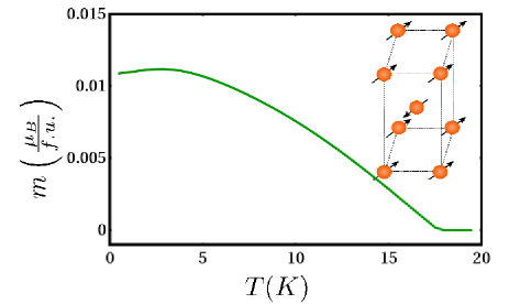
Figure 12: Predicted temperature dependence of the basal plane moment. Parameters used for this calculation are given in section.

Fig. (12) shows the temperature dependence of the magnetic moment calculated for a case where $D/T_{K}\approx 30$, for which $m_{\perp}(0)$ =0.015$\mu_{B}$, which is an upper bound for the predicted conduction electron moment. Neutron scattering measurements on URu₂Si₂ have placed bounds on the c-axis magnetization of the f-electrons using a momentum transfer $Q$ in the basal plane. Detection of an $m_{\perp}(0)$ carried by conduction electrons, with a small scattering form-factor requires high-resolution measurements with a c-axis momentum transfer. Recent high resolution neutron measurements to detect this small transverse moment have not detected a signal, and quote a bound on the f-component of the moment $|\vec{m}_{f}|<0.001\mu_{B}$. We discuss the implications of this result in section VI.2. We note that there have been reports from $\mu$SR and NMR measurementsAmitsuka03 ; Bernal04 of very small intrinsic basal plane fields in URu₂Si₂ comparable with this bound.

We can also examine the quadrupolar moment associated with the HO state. This is set by the expectation of the transverse components of the non-Kramers doublet,

$$Q_{x,y} \propto \langle\chi^{\dagger}_{\alpha}(\sigma_{x,y})_{\alpha\beta}\chi_{\beta}\rangle$$ (199)

$$= -T\sum_{i\omega_{n}}\sum_{\bf{k}}{\hbox{Tr}}\left[{\sigma}_{x,y}\mathcal{G}^{f}({\bf{k}},i\omega_{n})\tau_{1}\right].$$ (200)

If we expand this using the f-Green’s function from eq (125), we find

$$Q_{xy}\propto-\sum_{{\bf{k}}\eta}\frac{(E_{{\bf{k}}\eta}-\epsilon_{0{\bf{k}}})}{\prod_{\eta^{\prime}\neq\eta}(E_{{\bf{k}}\eta}-E_{{\bf{k}}\eta^{\prime}})}f(E_{{\bf{k}}\eta})\overrightarrow{\Delta}_{{\bf{k}}f+}.$$ (202)

.

The f-electron quadrupole moment (202) has an identical form to the conduction electron moment, (197), with $\epsilon\leftrightarrow\lambda$ everywhere, and the relevant form-factor is (124)

$$\overrightarrow{\Delta}_{{\bf{k}}f+} = -{\hbox{Tr}}\mathcal{V}^{\dagger}_{\bf{k}}\mathcal{V}_{\bf{k}}\tau_{1}\vec{\sigma}=-2{\hbox{Tr}}\left[\left(\mathcal{V}^{\dagger}_{6{\bf{k}}}\mathcal{V}_{7{\bf{k}}}+\mathcal{V}_{7{\bf{k}}}^{\dagger}\mathcal{V}_{6{\bf{k}}}\right)\vec{\sigma}\right]$$ (204)

.

which has a d-wave form-factor. This means that the summation over momentum vanishes, so that the staggered quadrupolar moments $Q_{x,y}$ must vanish. (Indeed, there would be no associated lattice distortion, even for a uniform hastatic order. ) As a d-wave quadrupole is an $L=4$-tupole, or “hexadecapole”, this means that like Haule and KotliarHaule09 , the hastatic order has staggered $(J_{x}J_{y}+J_{y}J_{x})(J_{x}^{2}-J_{y}^{2})$ hexadecapolar moments. However, unlike Haule and Kotliar, where the hexadecapolar moments are the primary order parameter (and thus of order one), here the hexadecapolar moments are a secondary effect of the composite hastatic order, and like the conduction electron moments, will be of order $T_{K}/D$. Given how difficult it is to observe large hexadecapolar moments, the hexadecapolar moments associated with hastatic order will almost certainly be unobservably small. By contrast, in the antiferromagnetic phase, the f-electrons develop a large c-axis magnetic moment.

We will return to the predicted basal plane moment in the HO phase of URu₂Si₂ in Section VI B. when we discuss recent experimental constraints.

VI Discussion and Open Questions

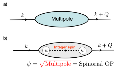
Figure 13: Schematic contrasting the multipolar and spinorial theories of Hidden order. (a) in a multipolar scenario, the heavy electrons Bragg diffract off a staggered spin or charge multipole (b) in the hastatic scenario, the development of a spinor hybridization opens up resonant scattering with a an integer spin state of the ion. The multipole is generated as a consequence of two spinorial scattering events. In this way, the Hastatic spinor order parameter can be loosely regarded as the square root of a multipole.

In summary, the key idea of the hastatic proposal for hidden order in URu₂Si₂ is that observation of heavy Ising quasiparticles implies the development of resonant scattering between half-integer spin electrons and integer spin local moments. It is perhaps useful to contrast the various staggered multipolar scenarios for the hidden order with the hastatic one proposed here. In the former, mobile f-electrons Bragg diffract off a multipolar density wave (see Fig 13 (a)), whereas in the latter, the multipole contains an internal structure, associated with the resonant scattering into an integer spin f-state. (see Fig 13 (b)). Hastatic order can thus be loosely regarded as the “square root” of a multipole order parameter,

$$\Psi\sim\sqrt{\hbox{multipole OP}}.$$ (205)

In fact, as we have seen the square of the hastatic order parameter breaks tetragonal symmetry, and is thus nematic (see Fig. 9.), with a director $\vec{n}=(n_{x},n_{y})$ of magnitude determined by the square of the hastatic order parameter,

$$(n_{x}+in_{y})\propto\psi^{*}_{\uparrow}\psi_{\downarrow}.$$ (206)

It can also be viewed to result from a symmetry-breaking Kondo effect between non-Kramers and Kramers doublets. Hastatic order should be present in any f-electron material whose unfilled f-shell contains a geometrically stabilized non-Kramers doublet, and we expect its realization in other $5f$ uranium and $4f$ praseodymium compounds. Praseodymium compounds are particularly promising tests for hastatic order, as the presence and nature of any non-Kramers doublets can be determined via inelastic neutron scattering. Any non-Kramers doublet Pr compound must order either magnetically or quadrupolarly or form hastatic order - there is no non-symmetry breaking option, as in Kramers materials.

VI.1 Broader Implications of Hastatic Order

At a microscopic level hastatic order demands a new kind of particle condensation, one that gives rise to a Landau order parameter that transforms under half-integer spin or double-group representations.Chandra14 Conventionally Landau theory in electronic systems is based on the formation and condensation of two-body bound-states. For example the development of a magnetic order parameter $\vec{M}(x)$ is given by the contraction

$$\stackrel{{\scriptstyle\mathclap{\displaystyle\raise-1.8pt\hbox{$\scriptscriptstyle|$}\mathrel{\mkern-9.0mu}\mathrel{{\bf\smash{{\phantom{-}\above 1.0pt\phantom{-}}}}}\mathrel{\mkern-6.0mu}\mathrel{{\bf\smash{{\phantom{-}\above 1.0pt\phantom{-}}}}}\mathrel{\mkern-6.0mu}\mathrel{{\bf\smash{{\phantom{-}\above 1.0pt\phantom{-}}}}}\mathrel{\mkern-6.0mu}\mathrel{{\bf\smash{{\phantom{-}\above 1.0pt\phantom{-}}}}}\mathrel{\mkern-9.0mu}\raise-1.8pt\hbox{$\scriptscriptstyle|$}}}}{{\psi^{\dagger}_{\alpha}(x)\psi_{\beta}(x)}}=\vec{\sigma}_{\alpha\beta}\cdot\vec{M}(x)$$ (207)

and s-wave superconductivity is based on the formation of spinless bosons

$$\stackrel{{\scriptstyle\mathclap{\displaystyle\raise-1.8pt\hbox{$\scriptscriptstyle|$}\mathrel{\mkern-9.0mu}\mathrel{{\bf\smash{{\phantom{-}\above 1.0pt\phantom{-}}}}}\mathrel{\mkern-6.0mu}\mathrel{{\bf\smash{{\phantom{-}\above 1.0pt\phantom{-}}}}}\mathrel{\mkern-6.0mu}\mathrel{{\bf\smash{{\phantom{-}\above 1.0pt\phantom{-}}}}}\mathrel{\mkern-6.0mu}\mathrel{{\bf\smash{{\phantom{-}\above 1.0pt\phantom{-}}}}}\mathrel{\mkern-9.0mu}\raise-1.8pt\hbox{$\scriptscriptstyle|$}}}}{{\psi_{\uparrow}(1)\psi_{\downarrow}(2)}}=-F(1-2),$$ (208)

where $F(1-2)=-\langle T\psi_{\uparrow}(1)\psi_{\downarrow}(2)\rangle$ is the anomalous Gor’kov Greens function that breaks the gauge system of the underlying system ( see Fig. 14 a). The take-home message from conventional two-body condensation is that when the two-body bound-state wavefunction carries a quantum number (e.g. charge or spin), a symmetry is broken. However under this scheme, all order parameters are bosons that carry integer spin.

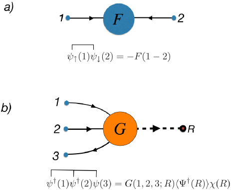
Figure 14: Schematic Feynman diagrams indicating (a) two-body (b) and three-body electronic bound-states where in the latter case spin indices have been suppressed for pedagogical simplicity.

Hastatic order carries half-integer spin and cannot develop via this mechanism. We are then led to the question of whether it is possible for Landau order parameters to transform under half-integer representations of the spin rotation group? At first sight this impossible for all order parameters are necessarily bosonic and bosons carry integer spin. However the connection between spin and statistics is strictly a relativistic idea that depends on the full Poincaré invariance of the vacuum. This invariance is lost in non-relativistic condensed matter systems,where high energy degrees of freedom are integrated out, suggesting the possibility of order parameters with half-integer spin that transform under double-group representations of the rotation group. Spinor order parameters involving “internal” quantum numbers are well known in the context of two-component Bose-Einstein condensates. The Higgs field of electroweak theory is also a two-component spinor. However in neither case does the spinor transform under the physical rotation group. Moreover it is not immediately obvious how such bound-states emerge within fermionic systems.

Hastatic order is a generalization of Landau’s order parameter concept to three-body bound-states. This is natural in heavy fermion systems since the conventional Kondo effect is the formation of a three-body bound state between a spin flip and a conduction electron. However here the three-body wavefunction carries no quantum number and thus is not an order parameter; this is why conventional Kondo behavior is associated with a crossover and not a true phase transition.

In the mean-field formulation of hastatic order,hastatic a spin-1/2 order parameter develops as a consequence of a factorization of a Hubbard operator that connect the Kramers and non-Kramers states; it is a tensor operator that corresponds to the three-body combination

$$X_{\alpha\sigma}(R)\equiv|f^{2}\alpha\rangle\langle f^{1}\sigma|=\Lambda_{\alpha\sigma}^{abc}(R;1,2,3)\psi^{\dagger}_{a}(1)\psi^{\dagger}_{b}(2)\psi_{c}(3),$$ (209)

where we have used the short-hand notation $1\equiv R_{1}$ etc. and

$$\Lambda_{\alpha\sigma}^{abc}(R;1,2,3)=\langle R_{1},a;R_{2},b|\hat{X}_{\alpha\sigma}(R)|R_{3},c\rangle$$ (210)

defines the overlap between the Hubbard operators and the bare electron states. In a simple model, this three body wavefunction is local, $\Lambda_{\alpha\sigma}^{abc}(R;1,2,3)=\Lambda_{\alpha\sigma}^{abc}\delta(R-1)\delta(R-2)\delta(R-3)$. The factorization of the Hubbard operator into a spin-1 fermion and a spin-1/2 boson

$$X_{\alpha\sigma}(R)\rightarrow\chi^{\dagger}_{\alpha}(R)\left\langle\Psi_{\sigma}(R)\right\rangle,$$ (211)

then represents a “fractionalization” of the three body operator. Written in terms of the microscopic electron fields, this becomes

$$\Lambda_{\alpha\sigma}^{abc}(R;1,2,3)\stackrel{{\scriptstyle\mathclap{\displaystyle\raise-1.8pt\hbox{$\scriptscriptstyle|$}\mathrel{\mkern-9.0mu}\mathrel{{\bf\smash{{\phantom{-}\above 1.0pt\phantom{-}}}}}\mathrel{\mkern-6.0mu}\mathrel{{\bf\smash{{\phantom{-}\above 1.0pt\phantom{-}}}}}\mathrel{\mkern-6.0mu}\mathrel{{\bf\smash{{\phantom{-}\above 1.0pt\phantom{-}}}}}\mathrel{\mkern-6.0mu}\mathrel{{\bf\smash{{\phantom{-}\above 1.0pt\phantom{-}}}}}\mathrel{\mkern-9.0mu}\raise-1.8pt\hbox{$\scriptscriptstyle|$}\mathrel{\mkern-11.0mu}\mathrel{{\bf\smash{{\phantom{-}\above 1.0pt\phantom{-}}}}}\mathrel{\mkern-9.0mu}\mathrel{{\bf\smash{{\phantom{-}\above 1.0pt\phantom{-}}}}}\mathrel{\mkern-9.0mu}\mathrel{{\bf\smash{{\phantom{-}\above 1.0pt\phantom{-}}}}}\mathrel{\mkern-9.0mu}\mathrel{{\bf\smash{{\phantom{-}\above 1.0pt\phantom{-}}}}}\mathrel{\mkern-9.0mu}\mathrel{{\bf\smash{{\phantom{-}\above 1.0pt\phantom{-}}}}}\mathrel{\mkern-9.0mu}\raise-1.8pt\hbox{$\scriptscriptstyle|$}}}}{{\psi^{\dagger}_{a}(1)\psi^{\dagger}_{b}(2)\psi_{c}(3)}} = \chi^{\dagger}_{\alpha}(R)\left\langle\phantom{\sum}\hskip-14.22636pt\Psi_{\sigma}(R)\right\rangle.$$ (212)

This expression can be inverted to give the three body contraction

$$\stackrel{{\scriptstyle\mathclap{\displaystyle\raise-1.8pt\hbox{$\scriptscriptstyle|$}\mathrel{\mkern-9.0mu}\mathrel{{\bf\smash{{\phantom{-}\above 1.0pt\phantom{-}}}}}\mathrel{\mkern-6.0mu}\mathrel{{\bf\smash{{\phantom{-}\above 1.0pt\phantom{-}}}}}\mathrel{\mkern-6.0mu}\mathrel{{\bf\smash{{\phantom{-}\above 1.0pt\phantom{-}}}}}\mathrel{\mkern-6.0mu}\mathrel{{\bf\smash{{\phantom{-}\above 1.0pt\phantom{-}}}}}\mathrel{\mkern-9.0mu}\raise-1.8pt\hbox{$\scriptscriptstyle|$}\mathrel{\mkern-11.0mu}\mathrel{{\bf\smash{{\phantom{-}\above 1.0pt\phantom{-}}}}}\mathrel{\mkern-9.0mu}\mathrel{{\bf\smash{{\phantom{-}\above 1.0pt\phantom{-}}}}}\mathrel{\mkern-9.0mu}\mathrel{{\bf\smash{{\phantom{-}\above 1.0pt\phantom{-}}}}}\mathrel{\mkern-9.0mu}\mathrel{{\bf\smash{{\phantom{-}\above 1.0pt\phantom{-}}}}}\mathrel{\mkern-9.0mu}\mathrel{{\bf\smash{{\phantom{-}\above 1.0pt\phantom{-}}}}}\mathrel{\mkern-9.0mu}\raise-1.8pt\hbox{$\scriptscriptstyle|$}}}}{{\psi^{\dagger}_{a}(1)\psi^{\dagger}_{b}(2)\psi_{c}(3)}} = \sum_{R}G_{abc}^{\alpha\sigma}(1,2,3;R)\chi^{\dagger}_{\alpha}(R)\left\langle\phantom{\sum}\hskip-14.22636pt\Psi_{\sigma}(R)\right\rangle,$$ (214)

where $G_{abc}^{\sigma\alpha}(1,2,3;R)=[\Lambda_{\sigma\alpha}^{abc}(R;1,2,3)]^{*}$ (see Fig. 14 b).

The asymmetric decomposition of a three-body fermion state into a binary combination of boson and fermion is a fractionalization process; if the boson carries a quantum number, when it condenses we have the phenomenon of “order parameter fractionalization”. Fractionalization is well-established for excitations of low dimensional systems, such the one-dimensional Heisenberg spin chain and the fractional quantum Hall effectJackiw76 ; Su79 ; Laughlin99 ; Castelnuovo12 , but order parameter fractionalization is a new concept. Unlike pair or exciton condensation, the hastatic order parameter transforms under a double-group representation of the underlying symmetry group, and thus represents a fundamentally new class of broken symmetries. We are currently investigating order parameter fractionalization beyond the realm of URu₂Si₂ . The proposed three-body bound-state has a nonlocal order parameter, and it may be possible to identify a dual theory with a local order parameter that breaks a global symmetry.

VI.2 Experimental Constraints and More Tests

Let us now return to the situation in URu₂Si₂ . As we discussed earlier, hastatic order leads to a predication of a basal-plane moment of order $\frac{T_{K}}{D}$, where $T_{K}$ and $D$ are the Kondo temperature and the band-width respectively. The transverse moment in our mean-field treatment has contributions from both conduction and f electrons, and the ratio $\frac{T_{K}}{D}$ is very sensitive to the degree of mixed valence of the $U$ ion. Our original calculation assumed $20\%$ 5$f^{3}$, leading to a predicted basal-plane moment of $0.01\mu_{B}$. Recent high-resolution neutron experimentsDas13 ; Metoki13 ; Ross14 with momentum transfer along the c-axis designed to detect this predicted transverse moment have placed a bound $\mu_{\perp}<0.0011\mu_{B}$ on the ordered transverse moment of the uranium ions, constraining it to be at best an order of magnitude smaller than what we predicted.

Clearly we need to reconsider our calculation of the transverse moment and understand why it is so small if not absent and we are currently exploring a number of possibilities:

• Fluctuations. Amplitude fluctuations of the hastatic order parameter are needed to describe the incoherent Fermi liquid observed to develop at temperatures well above $T_{HO}$ in optical, tunneling and thermodynamic measurements,Schmidt10 ; Aynajian10 ; Park11 ; Haraldsen11 and they will reduce the transverse moment. We note that various probes, including X-rays, $\mu$-spin resonance and NMRCaciuffo14 ; Amitsuka03 ; Bernal04 ; Takagi12 have consistently detected basal plane fields of order $0.5G$, consistent with the presence of a tiny in-plane moment.

• Uranium Valence. The predicted transverse moment is very sensitive to the $5$f valence, decreasing with increasing proximity to pure $5f^{2}$. More specifically it is proportional to the change in valence between $T_{HO}$ and the measurement temperature and thus is significantly smaller than the high-temperature mixed valency. It would be very helpful to have low temperature probes of the 5f-valence.

• Domains. X-ray,Caciuffo14 muon,Amitsuka03 torque magnetometryOkazaki11 , cyclotron resonanceMatsuda11 and NMR measurementsBernal04 ; Takagi12 that have indicated either a static moment or broken tetragonal symmetry were performed on small samples. By contrast, the neutron measurements that show no measurable moment use large samples Das13 ; Metoki13 ; Ross14 . The apparent inconsistency between these two sets of measurements may be due to domain formation of hidden order. Such domain structure could result from random pinningImry75 of the transverse moment by defects of random strain fields. The situation in URu₂Si₂ is somewhat analogous to that in Sr₂RuO₄, where there is evidence for broken time-reversal symmetry breaking with a measured Kerr effect and $\mu$SR to support chiral p-wave superconductivity, but no surface currents have yet been observed.Kallin12 Domains are an issue in this system too.

• x-y order and spin superflow. The current mean-field theory has the transverse hastatic vector $\Psi^{\dagger}\vec{\sigma}\Psi$ pointing in one of four possible directions at each site, corresponding to a four-state clock model. The tunneling barrier between these configurations is very small. When we expand the effective action as a function of $\phi$, the leading order anisotropy will have the form

  $$\Delta E(\phi)=E_{4}\cos 4\phi.$$ (216)

  where $E_{4\phi}$ determines the magnitude of the tunneling barrier. Now the anisotropic terms have the form $e^{\pm i4\phi}$, and since the $\phi$ dependence in ${\Psi}$ enters as $e^{\pm i\frac{\phi}{2}}$, the leading dependence of this term on ${\Psi}$ has the form

  $$E_{4}\sim T_{K}|{\Psi}|^{8}$$ (217)

  Now since $|{\Psi}|^{2}\sim\frac{T_{K}}{D}$, this implies that the tunneling barrier has magnitude

  $$E_{4}\sim T_{K}\left(\frac{T_{K}}{D}\right)^{4}$$ (218)

  In our theory we have estimated $T_{K}/D\sim 0.01$, so that the tunneling barrier is of order $10^{-8}$ times smaller than the Kondo temperature. In practice, the XY-like basal plane hastatic moments will be extremely weakly pinned, with large domain walls between $Z_{4}$ domains, with widths $\sim\frac{D}{T_{K}}\sim 100$ lattice spacings. To our knowledge, such nearly perfect XY order, which can lead to spin superflowchandracolemanlarkinsuperflow ; fomin ; borovik is completely unknown in magnetism: its only counterpart occurring in neutral superfluids. This opens the interesting possibility that the presence of persistent spin currents in the hastatic phase $j_{\hbox{spin}}\propto\nabla\phi$ give rise to a destruction of the staggered moment associated with hastatic order. By contrast, near the surfaces, where the tetragonal symmetry is broken, the $Z_{2}$ pinning is expected to be much greater. This might account for why large moments and broken tetragonal symmetry only appear in tiny crystals.

The central tenet of the hastatic proposal is that Ising quasiparticles are associated with the development of hidden order and there remain several tests of this aspect that can be made. In particular:

1. Giant Anisotropy in $\Delta\chi_{3}\propto\cos^{4}\theta$. In this measurement the temperature-dependence of the Ising anisotropy of the conduction fluid can be probed to confirm that it is associated with the development of hidden order.

2. dHvA on all the heavy Fermi surface pockets. Based on the upper-critical field results, we expect that the heavy quasiparticles in the $\alpha$ $\beta$ and $\gamma$ orbits will exhibit the multiple spin zeros of Ising quasiparticles but to date only the $\alpha$ orbits have been measured as a function of field orientation.

3. Spin zeros in the AFM phase? (Finite pressure) If the antiferromagnetic phase is also hastatic, then we expect the spin zeros to persist at finite pressures.

VI.3 Future Challenges

The observation of Ising quasiparticles in the hidden order state Brison95 ; Ohkuni99 ; Altarawneh11 ; Altarawneh12 represents a major challenge to our understanding of URu₂Si₂ ; to our knowledge this is the only example of such anisotropic mobile electrons, and as we have emphasized, completely unexpected for f-electrons in a tetragonal environment. As we have emphasized throughout this paper, Ising quasiparticles are the central motivation for the hastatic proposal, and a key question is whether this phenomenon can be described by other HO theories? In particular:

• Can band theory account for the $g(\theta)$ observed in URu₂Si₂ ? Recent advances in the understanding of orbital magnetizationXiao05 ; Thonhouser05 ; Xiao06 suggest it may be possible to compute the g-factor associated with conventional Bloch waves; in a strongly spin-orbit coupled system, the orbital contributions to the total energy in a magnetic field are significant. It would be particularly interesting to compare the $g(\theta)$ computed in a density functional treatment of URu₂Si₂ with that observed experimentally.

• Can other $5f^{2}$ theories account for the multiple spin zeroes and the upper bound $\Delta<1K$ on the spin degeneracy of the heavy fermion bands? In particular, is it possible to account for the observed spin zeros without invoking a non-Kramers $5f^{2}$ doublet?

We have benefitted from inspiring discussions with our colleagues who include C. Batista, C. Broholm, K. Haule, N. Harrison, G. Kotliar, P. A. Lee, G. Lonzarich, J. Mydosh, K. Ross and J. Schmalian. PC and PC are grateful to the hospitality of the Institute for the Theory of Condensed Matter, Karlsrule Instiute for Technology, the Centro Brasileiro de Pesquisas Fisicas (CBPF) and Trinity College, Cambridge where parts of this paper were written. PC and PC gratefully acknowledge the support of the Conselho Nacional de Desenvolvimento Científico e Tecnológico-CNPq Brasil (CBPF), supported by CAPES and FAPERJ grants CAPES - AUX–PE-EAE-705/2013 and FAPERJ - E-26/110.030/2013 during their stay. The three of us also acknowledge the hospitality of the Aspen Center for Physics, supported by National Science Foundation Grant No. PHYS-1066293 where we worked together on this project. This work was supported by the National Science Foundation grants NSF-DMR-1334428 (P. Chandra) and DMR-1309929 (P. Coleman), and by the Simons Foundation (R. Flint).

References

- (1) T.T.M. Palstra et al., “Superconducting and Magnetic Transitions in the Heavy-Fermion System ,” Phys. Rev. Lett. 55 2727-2730 (1985).
- (2) W. Schlabitz et al., “Superconductivity and Magnetic Order in a Strongly Interacting Fermi System: URu2Si2 ”, Z. Phys. B., 62, 171-177 (1986).
- (3) C. Broholm et al., “Magnetic excitations in the heavy-fermion superconductor URu2Si2 ,” Phys. Rev B. 43, 12809 (1991). Si2single crystals J. Appl. Phys. 70, 5791–5793 (1991).
- (4) M.B. Walter et al., “Nature of the order parameter in the Heavy-Fermion system URu2Si2 ,” Phys. Rev. Lett. 71, 2630 (1993).
- (5) S. Takagi et al., “No Evidence for “Small-Moment Antiferromagnetism” under Ambient Pressure in URu2Si2 : Single-Crystal 29Si NMR Study,” J. Phys. Soc. Jpn. 76, 033708 (2007).
- (6) H. Amitsuka, M. Sato, N. Metoki, M. Yokoyama, K. Kuwahara, T. Sakakibara, H. Morimoto, S. Kawarazaki, Y. Miyako, and J. A. Mydosh, Phys. Rev. Lett. 83, 5114 (1999).
- (7) H. Amitsuka et al., “Pressure-Temperature Phase Diagram of the Heavy-Electron Superconductor ,” J. Magn. Magn. Mater. 310, 214-220 (2007).
- (8) Nicholas P. Butch, Jason R. Jeffries, Songxue Chi, Juscelino Batista Leão, Jeffrey W. Lynn, and M. Brian Maple, “Antiferromagnetic critical pressure in URu2Si2 under hydrostatic conditions”, Phys. Rev. B 82, 060408 (R), (2010).
- (9) H. Amitsuka and T. Sakakibara,”Single Uranium-Site Properties of the Dilute Heavy Electron System ,” J. Phys. Soc. Japan 63 736-747 (1994).
- (10) K. Haule and G. Kotliar, “Arrested Kondo Effect and Hidden Order in ,” Nature Phys. 5, 796-799 (2009).
- (11) P. Santini and G. Amoretti, “Crystal Field Model of the Magnetic Properties of URu2Si2 ” Phys. Rev. Lett, 73, 1027-1030 (1994).
- (12) C. M. Varma and L. Zhu, “Helicity Order: Hidden Order Parameter in URu2Si2 ”, Phys. Rev. Lett. 96, 036405-036408 (2006).
- (13) C. Pépin, M. R. Norman, S. Burdin, and A. Ferraz, ”Modulated Spin Liquid: A New Paradigm for URu2Si2 ”, Phys. Rev. Lett. 106, 106601-106604 (2011).
- (14) Ting Yuan, Jeremy Figgins and Dirk K. Morr, “Hidden order transition in URu2Si2 : Evidence for the emergence of a coherent Anderson lattice from scanning tunneling spectroscopy”, Phys. Rev. B 86, 035129-035134 (2012).
- (15) Y. Dubi and A.V. Balatsky, “Hybridization Wave as the ‘Hidden Order’ in ,”, Phys. Rev. Lett. 106, 086401-086404 (2011).
- (16) S. Fujimoto, “Spin Nematic State as a Candidate of the Hidden Order Phase of , Phys. Rev. Lett. 106, 196407-196410 (2011).
- (17) H. Ikeda et al, “Emergent Rank-5 ‘Nematic’ Order in ”, Nature Physics 8, 528–533 (2012).
- (18) J. A. Mydosh and P. M. Oppeneer, “Colloquium: Hidden Order, Superconductivity and Magnetism – The Unsolved Case of URu2Si2 ”, Rev. Mod. Phys. 83, 1301–1322 (2011).
- (19) Premala Chandra, Piers Coleman and Rebecca Flint, “Hastatic order: a theory for the hidden order in URu2Si2”, Nature, 493, 621-626 (2013).
- (20) R. Flint, P. Chandra and P. Coleman, “Hidden and Hastatic orders in URu2Si2 ”, J. Phys. Soc. Jpn. 83, 061003 (2014).
- (21) P. Chandra, P. Coleman and R. Flint, “Ising Quasiparticles and Hidden Order in URu2Si2 ” Phil. Mag 94:32-33, 3803 - 3819 (2014).
- (22) H. Ohkuni, Y. Inada, Y. Tokiwa, K. Sakurai, R. Settai , T. Honma, Y. Haga, E. Yamamoto, Y. Obarnuki , H. Yamagami, S. Takahashi & T. Yanagisawa, “Fermi surface properties and de Haas-van Alphen oscillation in both the normal and superconducting mixed states of URu2Si2 ”, Phil. Mag. B 79, 1045 (1999).
- (23) M. M. Altarawneh, N. Harrison, S. E. Sebastian, L. Balicas, P. H. Tobash, J. D. Thompson, F. Ronning, and E. D. Bauer Phys. Rev. Lett. 106, 146403-146416 (2011).
- (24) J. P. Brison et al, “Anisotropy of the upper critical field in URu2Si2 and FFLO state in antiferromagnetic superconductors”, Physica C 250, 128-138 (1995).
- (25) M. M. Altarawneh et al. , “Superconducting pairs with extreme uniaxial anisotropy in URu2Si2 ” Phys. Rev. Lett. 108, 066407-066410 (2012).
- (26) T. T. M. Palstra, A. A. Menvosky and J. A. Mydosh, “Anisotropic electrical resistivity of the magnetic heavy-fermion superconductor URu2Si2 ”, Phys.Rev. B, 33, 6528 (1986).
- (27) Y.J. Jo et al.,”Field-Induced Fermi Surface Reconstruction and Adiabatic Continuity between Antiferromagnetism and the Hidden-Order State in ,” Phys. Rev. Lett. 98, 166404-165407 (2007).
- (28) A. Villaume et al., “Signature of Hidden Order in Heavy Fermion Superconductor : Resonance at the wave vector ,”Phys. Rev. B 78 5114-5117 (2008).
- (29) E. Hassinger et al, “Similarity of the Fermi Surface in the Hidden Order State and in the Antiferromagnetic State of ,” Phys. Rev. Lett. 105, 216409-216412 (2010).
- (30) K. Haule and G. Kotliar, “Complex Landau-Ginzburg Theory of the Hidden Order in ,” Eur. Lett. 89 57006:p1-57006:p6 (2010).
- (31) A.P. Ramirez et al., “Nonlinear Susceptibility as a Probe of Tensor Spin Order in ,”, Phys. Rev. Lett. 68, 2680-2683 (1992).
- (32) F.J. Ohkawa and H. Shimizu, “Quadrupole and Dipole Orders in ,” J. Phys: Cond. Mat. 11, L519-L524 (1999).
- (33) R. Flint, P. Chandra and P. Coleman, “Basal-Plane Nonlinear Susceptibility: A Direct Probe of the Single-Ion Physics in URu2Si2”, Phys. Rev. B 86, 155155-155160(2012).
- (34) E. A. Goremychkin, R. Osborn, B. D. Rainford, and A. P. Murani, “Evidence for Anisotropic Kondo Behavior in Ce0.8La0.2Al3,” Phys. Rev. Lett. 84, 2211 (2000).
- (35) A.E. Sikkema, W.J.L. Buyers, I. Affleck and J.Gan, “Ising-Kondo lattice with transverse field: A possible f-moment Hamiltonian for URu2Si2 ,” Phys. Rev. B 54, 9322 (1996).”
- (36) D. L. Cox and A. Zawadowski, “Exotic Kondo Effects in Metals”, Taylor & Francis, London. (2002).
- (37) U. Nagel et al., “Optical spectroscopy shows that the normal state of URu2Si2 is an anomalous Fermi liquid”, Proc. National Academy Science, 109, 1916-1965 (2012).
- (38) A. R. Schmidt et al., “Imaging the Fano lattice to ‘hidden order’ transition in URu2Si2 ”, Nature 465, 570-576 (2010).
- (39) P. Aynajian et al., “Visualizing the Formation of the Kondo Lattice and the Hidden Order in URu2Si2 ”, PNAS 107, 10383-10388 (2010).
- (40) W.K. Park et al, “Fano Resonance and Hybridization Gap in Kondo Lattice ”, Phys. Rev. Lett. 108, 246403-24646 (2012).
- (41) P. Coleman, “A New approach to the Mixed Valence Problem”, Phys. Rev. B 29, 3035-3044 (1984)
- (42) D.L. Cox and M. Jarrell, “The Two-Channel Kondo route to non-Fermi liquids,” J. Phys. Cond. Mat.8 9825-9853 (1996).
- (43) P. Coleman, A. M. Tsvelik, N. Andrei & H. Y. Kee, “Co-operative Kondo effect in the two-channel Kondo lattice” Phys. Rev. B 60, 3608-3628 (1999).
- (44) S. Hoshino, J. Otsuki and Y. Kuramoto, “Diagonal Composite Order in a Two-Channel Kondo Lattice” Phys. Rev. Lett. 107, 247202-247205 (2011).
- (45) C. Bolech and N. Andrei, “Solution of the Two-Channel Anderson Impurity Model: Implications for the Heavy Fermion UBe13” , Phys. Rev. Lett., 88, 237206-237209 (2002).
- (46) P. Coleman, J. B. Marston and A. J. Schofield, “Transport anomalies in a simplified model for a heavy-electron quantum critical point, Phys. Rev. B 72, 245111-245116 (2003).
- (47) C. Broholm et al., “Magnetic excitations in the heavy-fermion superconductor ,” Phys. Rev B. 43, 12809-12822 (1991).
- (48) C.R. Wiebe et al, “Gapped Itinerant Spin Excitations Account for Missing Entropy in the Hidden Order State of ,” Nature Physics 3, 96-99 (2007).
- (49) P. G. Niklowitz, S. Dunsiger, C. Pfleiderer, P. Link, A. Schneidewind, E. Faulhaber, M. Vojta, Y.-K. Huang, and J. A. Mydosh, “Role of commensurate and incommensurate low-energy excitations in the paramagnetic to hidden-order transition of URu2Si2 ”, arXiv:1110.5599 (2011).
- (50) N. Kanchanavavatee et al, “Twofold enhancement of the hidden-order/large-moment antiferromagnetic phase boundary in the URu2-xFexSi2 system”, Phys. Rev. B 84, 245122 (2011).
- (51) P. M. Oppeneer, J. Rusz, S. Elgazzar, M.-T. Suzuki, T. Durakiewicz, and J. A. Mydosh Phys. Rev. B 82, 205103 (2010).
- (52) J. C. Slater and G. F. Koster, “Simplified LCAO Method for the Periodic Potential Problem”, Phys. Rev. 94, 1498-1524, (1954).
- (53) R. Okazaki et al., “Rotational Symmetry Breaking in the Hidden Order Phase of ”, Science 331 439-442 (2011).
- (54) A. F. Santander-Syro et al., “Fermi-surface instability at the ’hidden order’ transition of ” Nature Physics 5, 637 - 641 (2009).
- (55) P. Haen , F. Lapierre, P. Lejay, J. Voiron, J. Magnetism and Magnetic Materials 116, 108-110 (1992).
- (56) J.T. Haraldsen et al., Phys. Rev. B 84, 214410 (2011).
- (57) R. Flint, M. Dzero & P. Coleman, Nat. Phys. 4, 643 (2008).
- (58) N. Andrei and C. Destri, “Solution of the Multichannel Kondo Problem”, Phys. Rev. Lett., 52, 364 (1984).
- (59) A. M. Tsvelik and P. B. Wiegmann, “Exact solution of the multichannel Kondo problem, scaling, and integrability”, J.Stat. Phys. 38, 125 (1985).
- (60) V. J. Emery and S. Kivelson, “Mapping of the two-channel Kondo problem to a resonant-level model”, Phys. Rev. B 46, 10812 (1992).
- (61) M. Jaime, K. H. Kim, G. Jorge, S. McCall, and J. A. Mydosh, “High Magnetic Field Studies of the Hidden Order Transition in URu2Si2,” Phys. Rev. Lett. 89, 287201 (2002).
- (62) M. Maltseva, M. Dzero and P. Coleman, “Electron Cotunneling into a Kondo Lattice”, Physical Review Letters 103, 206402 (2009).
- (63) A. P. Ramirez, P. Coleman, P. Chandra, E. Br uck, A. A. Menovsky, Z. Fisk, and E. Bucher, “Nonlinear susceptibility as a probe of tensor spin order in URu2Si2 ”, Phys. Rev. Lett.68, 2680 (1992).
- (64) P. Chandra et al., Physica B, 199 & 200 426 (1994).
- (65) P.W. Anderson, “Localized magnetic states in metals”, Phys. Rev. 124,41-53 (1961).
- (66) H. Amitsuka et al., “Inhomogeneous magnetism in URu2Si2 studied by muon spin relaxation under high pressure,” Physica B 326, 418-421 (2003).
- (67) O.O. Bernal et al., “Ambient Pressure 99Ru NMR in : Internal Field Anisotropy,” J. Mag. Magn. Mat. 272, E59-60 (2004).
- (68) R. Jackiw and C. Rebbi, Phys. Rev. D 13 3398 (1976).
- (69) W.P. Su, J.R. Schrieffer and A.J. Heeger, Phys. Rev. Lett. 42 1698 (1979).
- (70) R.B. Laughlin, Rev. Mod. Phys. 71, 863 (1999).
- (71) C Castelnovo, R. Moessner and S.L. Sondhi, Ann. Rev. Cond. Mat. 3 35 (2012).
- (72) P. Das et al., New J. Phys. 15, 053031 (2013).
- (73) N. Metoki et al., J. Phys. Soc. Jpn. 82, 055004 (2013).
- (74) K.A. Ross, L. Harriger, Z. Yamani, W. J. L. Buyers, J. D. Garrett, A. A. Menovsky, J. A. Mydosh and C. L. Broholm, arXiv:1402.2689 (2014).
- (75) R. Caciuffo, Private Communication.
- (76) Shigeru Takagi, Shu Ishihara, Makato Yokoyama and Hiroshi Amitsuka, “Symmetry of the Hidden Order in URu2Si2 from Nuclear Magnetic Resonance Studies”, J. Phys. Soc. Jpn. 81, 114710 (2012).
- (77) S. Tonegawa et al, “Cyclotron Resonance in the Hidden-Order Phase of URu2Si2 ” PRL 109, 036501-036504 (2012)
- (78) Y. Imry and S.-K. Ma, Phys. Rev. Lett. 35, 1399 (1975).
- (79) C. Kallin, Rep. Prog. Phys. 75, 042501 (2012).
- (80) P. Chandra , P. Coleman & A. I. Larkin, , “Quantum fluids approach to Frustrated Heisenberg Models”, Journal of Condensed Matter Physics, 2 7933, (1990).
- (81) I. A. Fomin, Long-lived induction signal and spatially nonuniform spin precession in 3He-B, Pisma Zh. Eksp. Teor. Fiz 40, 260 (1984)[JETP Lett. 40, 1037 (1984).
- (82) A. S. Borovik-Romanov, Yu. M. Bunkov, V. V. Dmitriev, Yu. M. Mukharskii and K. Flachbart, “Experimental study of separation of magnetization precession in 3He- into two magnetic domains, Zh. Eksp Teor Fiz 87, 2025-2038 (1985)[ Sov. Phys JETP, 61, 1199 (1985)].
- (83) J.P. Brison , N. Keller , A. Vernière , P. Lejay , L. Schmidt, A. Buzdin, J. Flouquet , S.R. Julian and G.G. Lonzarich, Physica C 250, 128-138 (1995).
- (84) M. M. Altarawneh, N. Harrison, G. Li, L. Balicas, P. H. Tobash, F. Ronning, and E. D. Bauer, Phys. Rev. Lett. 108, 066407-066410 (2012).
- (85) D. Xiao, J. Shi, and Q. Niu, Phys. Rev. Lett. 95, 137204 (2005).
- (86) T. Thonhauser, D. Ceresoli, D. Vanderbilt, and R. Resta, Phys. Rev. Lett. 95, 137205 (2005).
- (87) D. Xiao, Y. Yao, Z. Fang and Q. Niu, Phys. Rev. Lett. 97, 026603 (2006).