Sobolev inequalities in arbitrary domains

Abstract

A theory of Sobolev inequalities in arbitrary open sets in ${{\mathbb{R}}^{n}}$ is established. Boundary regularity of domains is replaced with information on boundary traces of trial functions and of their derivatives up to some explicit minimal order. The relevant Sobolev inequalities involve constants independent of the geometry of the domain, and exhibit the same critical exponents as in the classical inequalities on regular domains. Our approach relies upon new representation formulas for Sobolev functions, and on ensuing pointwise estimates which hold in any open set.

1 Introduction

$\mathcal{a}$ $\mathcal{b}$

The aim of this paper is to develop a theory of Sobolev embeddings, of any order $m\in\mathbb{N}$, in arbitrary open sets $\Omega$ in ${{\mathbb{R}}^{n}}$. As usual, by an $m$-th order Sobolev embedding we mean an inequality between a norm of the $h$-th order weak derivatives ($0\leq h\leq m-1$) of any $m$ times weakly differentiable function in $\Omega$ in terms of norms of some of its derivatives up to the order $m$.

The classical theory of Sobolev embeddings involves ground domains $\Omega$ satisfying suitable regularity assumptions. For instance, a formulation of the original theorem by Sobolev reads as follows. Assume that $\Omega$ is a bounded domain satisfying the cone property, $m\in\mathbb{N}$, $1<p<\tfrac{n}{m}$, and $\mathcal{F}(\cdot)$ is any continuous seminorm in $W^{m,p}(\Omega)$ which does not vanish on any polynomial of degree not exceeding $m-1$. Then there exists a constant $C=C(\Omega)$ such that

(1.1) $$\|u\|_{L^{\frac{np}{n-mp}}(\Omega)}\leq C\big{(}\|\nabla^{m}u\|_{L^{p}(\Omega)}+\mathcal{F}(u)\big{)}$$

for every $u\in W^{m,p}(\Omega)$. Here, $W^{m,p}(\Omega)$ denotes the usual Sobolev space of those functions in $\Omega$ whose weak derivatives up to the order $m$ belong to $L^{p}(\Omega)$, and $\nabla^{m}u$ stands for the vector of all (weak) derivatives of $u$ of order $m$.

It is well known that standard Sobolev embeddings are spoiled in presence of domains with “bad” boundaries. In particular, inequalities of the form (1.1) do not hold, at least with the same critical exponent $\frac{np}{n-mp}$, in irregular domains. This is the case, for instance, of domains with outward cusps. A theory of Sobolev embeddings, including possibly irregular domains, was initiated in the papers [Ma1] and [Ma3], and is systematically exposed in the monograph [Ma8], where classes of Sobolev inequalities are characterized in terms of geometric properties of the domain. Specifically, they are shown to be equivalent to either isoperimetric or isocapacitary inequalities relative to the domain. The interplay between the geometry of the domain and Sobolev inequalities, even in frameworks more general than the Euclidean one, has over the years been the subject of extensive investigations, along diverse directions, by a number of authors. Their results are the object of a rich literature, which includes the papers [AFT, Au, BCR, BL, BWW, BH2, BL, BK, BK1, Che, Ci1, Ci2, CFMP, CP, EKP, EFKNT, Gr, HaKo, HS, KP, KM, Kl, Kol, LPT, LYZ, Mi, Mo, Ta, Zh] and the monographs [BZ, CDPT, Cha, He, Ma8, Sa]. An updated bibliography on the area of Sobolev type inequalities can be found in [Ma8].

In order to remove any a priori regularity assumption on $\Omega$, we consider Sobolev inequalities from an unconventional perspective. The underling idea of our results is that suitable information on boundary traces of trial functions can replace boundary regularity of the domain in Sobolev inequalities.

The inequalities that will be established have the form

(1.2) $$\|\nabla^{h}u\|_{Y(\Omega,\mu)}\leq C\big{(}\|\nabla^{m}u\|_{X(\Omega)}+\mathcal{N}_{\partial\Omega}(u)\big{)},$$

where $m\in\mathbb{N}$, $h\in\mathbb{N}_{0}$, $\|\cdot\|_{X(\Omega)}$ is a Banach function norm on $\Omega$ with respect to Lebesgue measure $\mathcal{L}^{n}$, $\|\cdot\|_{Y(\Omega,\mu)}$ is a Banach function norm with respect to a possibly more general measure $\mu$, and $\mathcal{N}_{\partial\Omega}(\cdot)$ is a (non-standard) seminorm on $\partial\Omega$, depending on the trace of $u$, and of its derivatives up to the order $\big{[}\tfrac{m-1}{2}\big{]}$. Here, $\mathbb{N}_{0}=\mathbb{N}\cup\{0\}$, and $[\cdot]$ stands for integer part. Moreover, $\nabla^{0}u$ stands just for $u$, and we shall denote $\nabla^{1}u$ also by $\nabla u$.

Some distinctive features of the inequalities to be presented can be itemized as follows:

$\bullet$ No regularity on $\Omega$ is a priori assumed. In particular, the constants in (1.2) are independent of the geometry of $\Omega$.

$\bullet$ The critical Sobolev exponents, or, more generally, the optimal target norms, are the same as in the case of regular domains.

$\bullet$ The order $\big{[}\tfrac{m-1}{2}\big{]}$ of the derivatives, on which the seminorm $\mathcal{N}_{\partial\Omega}(\cdot)$ depends, is minimal for an inequality of the form (1.2) to hold without any additional assumption on $\Omega$.

A first-order Sobolev inequality on arbitrary domains $\Omega$ in ${{\mathbb{R}}^{n}}$ of the form (1.2), where $X(\Omega)=L^{p}(\Omega)$, $Y(\Omega,\mu)=L^{q}(\Omega)$, and $\mathcal{N}_{\partial\Omega}(\cdot)=\|\cdot\|_{L^{r}(\partial\Omega)}$, with $1\leq p<n$, $r\geq 1$ and $q=\min\{\tfrac{rn}{n-1},\tfrac{np}{n-p}\}$ was established in [Ma1] via isoperimetric inequalities. Sobolev inequalities of this kind, but still involving only first-order derivatives and Lebesgue measure, have received a renewed attention in recent years. In particular, the paper [MV1] makes use of mass transportation techniques to address the problem of the optimal constants for $p\in(1,n)$, the problem when $p=1$ having already been solved in [Ma1]. Sharp constants in inequalities in the borderline case when $p=n$ are exhibited in [MV2].

In the present paper, we develop a completely different approach, which not only enables us to establish arbitrary-order inequalities, which cannot just be derived via iteration of first-order ones, but also augments the first-order theory, in that more general measures and norms are allowed.

Our point of departure is a new pointwise estimate for functions, and their derivatives, on arbitrary – possibly unbounded and with infinite measure – domains $\Omega$. Such estimate involves a novel class of double-integral operators, where integration is extended over $\Omega\times\mathbb{S}^{n-1}$. The relevant operators act on a kind of higher-order difference quotients of the traces of functions and of their derivatives on $\partial\Omega$.
In view of applications to norm inequalities, the next step calls for an analysis of boundedness properties of these operators in function spaces. To this purpose, we prove their boundedness between optimal endpoint spaces. In combination with interpolation arguments based on the use of Peetre $K$-functional, these endpoint results lead to pointwise bounds, for Sobolev functions, in rearrangement form. As a consequence, Sobolev inequalities on an arbitrary $n$-dimensional domain are reduced to considerably simpler one-dimensional inequalities for Hardy type operators.

With this apparatus at disposal, we are able to establish inequalities involving Lebesgue norms, with respect to quite general measures, as well as Yudovich-Pohozaev-Trudinger type inequalities in exponential Orlicz spaces for limiting situations. The compactness of corresponding Reillich-Kondrashov type embeddings, with subcritical exponents, is also shown. Inequalities for other rearrangement-invariant norms, such as Lorentz and Orlicz norms, could be derived. However, in order to avoid unnecessary additional technical complications, this issue is not addressed here.

The paper is organized as follows. In the next section we offer a brief overview of some Sobolev type inequalities, in basic cases, which follow from our results, and discuss their novelty and optimality. Section 3 contains some preliminary definitions and results. The statement of our main results starts with Section 4, which is devoted to our key pointwise inequalities for Sobolev functions on arbitrary open sets. Estimates in rearrangement form are derived in the subsequent Section 5. In Section 6, Sobolev type inequalities in arbitrary open sets are shown to follow via such estimates. Examples which demonstrate the sharpness of our results are exhibited in Section 7. In particular, Example 7.4 shows that inequalities of the form (1.2) may possibly fail if $\mathcal{N}_{\partial\Omega}(u)$ only depends on derivatives of $u$ on $\partial\Omega$ up to an order smaller than $[\frac{m-1}{2}]$. Finally, in the Appendix, some new notions, which are introduced in the definitions of the seminorms $\mathcal{N}_{\partial\Omega}(\cdot)$, are linked to classical properties of Sobolev functions.

2 A taste of results

In order to give an overall idea of the content of this paper, we enucleate hereafter a few basic instances of the inequalities that can be derived via our approach.

We begin with two examples which demonstrate that our conclusions lead to new results also in the case of first-order inequalities, namely in the case when $m=1$ in (1.2).
Let $\Omega$ be any open set in ${{\mathbb{R}}^{n}}$, and let $\mu$ be a Borel measure on $\Omega$ such that $\mu(B_{r}\cap\Omega)\leq Cr^{\alpha}$ for some $C>0$, and $\alpha\in(n-1,n]$, and for every ball $B_{r}$ radius $r$. Clearly, if $\mu=\mathcal{L}^{n}$, then this condition holds with $\alpha=n$.
Assume that $1<p<n$ and $r>1$, and let $s=\min\{\tfrac{r\alpha}{n-1},\tfrac{\alpha p}{n-p}\}$. Then

(2.1) $$\|u\|_{L^{s}(\Omega,\mu)}\leq C\big{(}\|\nabla u\|_{L^{p}(\Omega)}+\|u\|_{L^{r}(\partial\Omega)}\big{)}$$

for some constant $C$ and every function $u$ with bounded support, provided that $\mathcal{L}^{n}(\Omega)<\infty$, $\mu(\Omega)<\infty$ and ${\mathcal{H}}^{n-1}(\partial\Omega)<\infty$. Here, ${\mathcal{H}}^{n-1}$ denotes the $(n-1)$-dimensional Hausdorff measure. In particular, if $r=\tfrac{p(n-1)}{n-p}$, and hence $s=\tfrac{\alpha p}{n-p}$, then (2.1) holds even if the assumption on the finiteness of these measures is dropped; in this case, the constant $C$ depends only on $n$. Inequality (2.1) follows via a general principle contained in Theorem 6.1, Section 6. It extends a version of the Sobolev inequality for measures, on regular domains [Ma8, Theorem 1.4.5]. It also augments, at least for $p>1$, the results for general domains of [Ma1] and [MV1], whose approach is confined to norms evaluated with respect to the Lebesgue measure. Let us point out that, by contrast, our method, being based on representation formulas, need not lead to optimal inequalities for $p=1$.
Consider now the borderline case corresponding to $p=n$. As a consequence of Theorem 6.1 again, one can show that

(2.2) $$\|u\|_{\exp L^{\frac{n}{n-1}}(\Omega,\mu)}\leq C\Big{(}\|\nabla u\|_{L^{n}(\Omega)}+\|u\|_{\exp L^{\frac{n}{n-1}}(\partial\Omega)}\Big{)},$$

for some constant $C$ and every function $u$ with bounded support, provided that $\mathcal{L}^{n}(\Omega)<\infty$, $\mu(\Omega)<\infty$ and ${\mathcal{H}}^{n-1}(\partial\Omega)<\infty$. Here, $\|\cdot\|_{\exp L^{\frac{n}{n-1}}(\Omega,\mu)}$ and $\|\cdot\|_{\exp L^{\frac{n}{n-1}}(\partial\Omega)}$ denote norms in Orlicz spaces of exponential type on $\Omega$ and $\partial\Omega$, respectively. Inequality (2.2) on the one hand extends the Yudovich-Pohozaev-Trudinger inequality to possibly irregular domains; on the other hand, it improves a result of [MV2], where estimates for the weaker norm in $\exp L(\Omega)$ are established, and just for the Lebesgue measure.

Let us now turn to higher-order inequalities. Focusing, for the time being, on second-order inequalities may help to grasp the quality and sharpness of our conclusions in this framework. In the remaining part of this section, we thus assume that $m=2$ in (1.2); we also assume, for simplicity, that $\mu=\mathcal{L}^{n}$.

First, assume that $h=0$. Then we can prove (among other possible choices of the exponents) that, if $1<p<\tfrac{n}{2}$, then

(2.3) $$\|u\|_{L^{\frac{pn}{n-2p}}(\Omega)}\leq C\big{(}\|\nabla^{2}u\|_{L^{p}(\Omega)}+\|u\|_{\mathcal{V}^{1,0}L^{\frac{p(n-1)}{n-p}}(\partial\Omega)}+\|u\|_{L^{\frac{p(n-1)}{n-2p}}(\partial\Omega)}\big{)},$$

for some constant $C=C(p,n)$, in particular independent of $\Omega$, and every function $u$ with bounded support. Note that $\tfrac{pn}{n-2p}$ is the same critical Sobolev exponent as in the case of regular domains. Here, $\|\cdot\|_{\mathcal{V}^{1,0}L^{r}(\partial\Omega)}$ denotes, for $r\in[1,\infty]$, the seminorm given by

(2.4) $$\|u\|_{\mathcal{V}^{1,0}L^{r}(\partial\Omega)}=\inf_{g}\|g\|_{L^{r}(\partial\Omega)},$$

where the infimum is taken among all Borel functions $g$ on $\partial\Omega$ such that

(2.5) $$|u(x)-u(y)|\leq|x-y|(g(x)+g(y))\quad\hbox{for ${\mathcal{H}}^{n-1}$-a.e. $x,y\in\partial\Omega$,}$$

and $L^{r}(\partial\Omega)$ denotes a Lebesgue space on $\partial\Omega$ with respect to the measure ${\mathcal{H}}^{n-1}$. The function $g$ appearing in (2.5) is an upper gradient, in the sense of [Ha], for the restriction of $u$ to $\partial\Omega$, endowed with the metric inherited from the Euclidean metric in ${{\mathbb{R}}^{n}}$, and with the measure ${\mathcal{H}}^{n-1}$. In [Ha], a definition of this kind, and an associated seminorm given as in (2.4), were introduced to define first-order Sobolev type spaces on arbitrary metric measure spaces. In the last two decades, various notions of upper gradients and of Sobolev spaces of functions defined on metric measure spaces, have been the object of investigations and applications. They constitute the topic of a number of papers and monographs, including [AT, BB, FHK, HaKo, Hei, HeKo, Kos].
Let us emphasize that, although the new term $\|u\|_{\mathcal{V}^{1,0}L^{\frac{p(n-1)}{n-p}}(\partial\Omega)}$ on the right-hand side of (2.3) can be dropped when $\Omega$ is a regular, say Lipschitz, domain, it is indispensable in an arbitrary domain. This can be shown by a domain as in Figure 1 (see Example 7.1, Section 7).

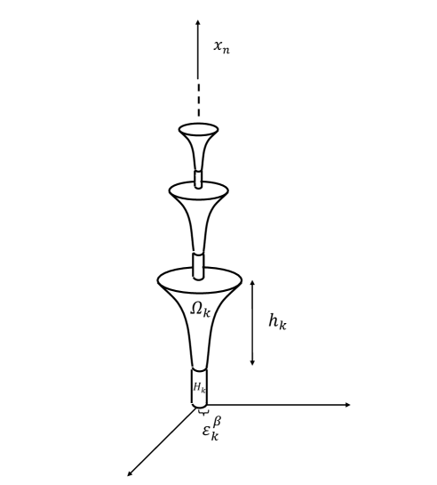
Figure 1: Example 7.1, Section 7

As in the case of regular domains, if $p>\tfrac{n}{2}$, then the Lebesgue norm on the left-hand side of (2.3) can be replaced by the norm in $L^{\infty}$. Indeed, if $r>n-1$, then

(2.6) $$\|u\|_{L^{\infty}(\Omega)}\leq C\big{(}\|\nabla^{2}u\|_{L^{p}(\Omega)}+\|u\|_{\mathcal{V}^{1,0}L^{r}(\partial\Omega)}+\|u\|_{L^{\infty}(\partial\Omega)}\big{)}$$

for any open set $\Omega$ such that $\mathcal{L}^{n}(\Omega)<\infty$ and ${\mathcal{H}}^{n-1}(\partial\Omega)<\infty$, for some constant $C$, and for any function $u$ with bounded support. In particular, the constant $C$ depends on $\Omega$ only through $\mathcal{L}^{n}(\Omega)$ and ${\mathcal{H}}^{n-1}(\partial\Omega)$.

In the limiting situation when $n\geq 3$, $p=\tfrac{n}{2}$ and $r>n-1$, a Yudovich-Pohozaev-Trudinger type inequality of the form

(2.7) $$\|u\|_{\exp L^{\frac{n}{n-2}}(\Omega)}\leq C\big{(}\|\nabla^{2}u\|_{L^{\frac{n}{2}}(\Omega)}+\|u\|_{\mathcal{V}^{1,0}L^{r}(\partial\Omega)}+\|u\|_{\exp L^{\frac{n}{n-2}}(\partial\Omega)}\big{)}$$

holds for some constant $C$ independent of the regularity of $\Omega$, and every function $u$ with bounded support, provided that $\mathcal{L}^{n}(\Omega)<\infty$ and ${\mathcal{H}}^{n-1}(\partial\Omega)<\infty$. The norms $\|\cdot\|_{\exp L^{\frac{n}{n-2}}(\Omega)}$ and $\|\cdot\|_{\exp L^{\frac{n}{n-2}}(\partial\Omega)}$ are the same exponential norms appearing in the Yudovich-Pohozaev-Trudinger inequality on regular domains, and in its boundary trace counterpart.

Consider next the case when still $m=2$ in (1.2), but $h=1$. Then one can infer from our estimates that, if $1<p<n$ and $r\geq 1$, and $\Omega$ is any open set with $\mathcal{L}^{n}(\Omega)<\infty$ and ${\mathcal{H}}^{n-1}(\partial\Omega)<\infty$, then

(2.8) $$\|\nabla u\|_{L^{q}(\Omega)}\leq C\big{(}\|\nabla^{2}u\|_{L^{p}(\Omega)}+\|u\|_{\mathcal{V}^{1,0}L^{r}(\partial\Omega)}\big{)}$$

for some constant $C$ independent of the geometry of $\Omega$, and every function $u$ with bounded support, where

(2.9) $$q=\min\big{\{}\tfrac{rn}{n-1},\tfrac{np}{n-p}\big{\}}.$$

In particular, if $r=\tfrac{p(n-1)}{n-p}$, and hence $q=\frac{np}{n-p}$, then the constant $C$ in (2.8) depends only on $n$ and $p$.
Inequality (2.8) is optimal under various respects. For instance, if $\Omega$ is regular, then, as a consequence of (1.1), the seminorm $\|u\|_{\mathcal{V}^{1,0}L^{r}(\partial\Omega)}$ can be replaced just with $\|u\|_{L^{r}(\partial\Omega)}$ on the right-hand side. By contrast, a domain $\Omega$ as in Figure 2 shows that this is impossible for every $q\in[1,\tfrac{np}{n-p}]$, whatever $r$ is – see Example 7.2, Section 7.

Figure 2: Example 7.2, Section 7

The question of the optimality of the exponent $q$ given by (2.9) can also be raised. The answer is affirmative. Actually, domains like that of Figure 3 show that such exponent $q$ is the largest possible in (2.8) if no regularity is imposed on $\Omega$ (Example 7.3, Section 7).

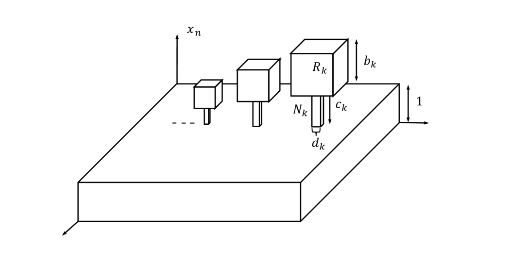
Figure 3: Example 7.3, Section 7

When $p>n$, inequality (2.8) can be replaced with

(2.10) $$\|\nabla u\|_{L^{\infty}(\Omega)}\leq C\big{(}\|\nabla^{2}u\|_{L^{p}(\Omega)}+\|u\|_{\mathcal{V}^{1,0}L^{\infty}(\partial\Omega)}\big{)},$$

for some constant $C$ independent of the regularity of $\Omega$, and every function $u$ with bounded support, provided that $\mathcal{L}^{n}(\Omega)<\infty$ and ${\mathcal{H}}^{n-1}(\partial\Omega)<\infty$.

Finally, in the borderline case corresponding to $p=n$, an exponential norm is involved again. Under the assumption that $\mathcal{L}^{n}(\Omega)<\infty$ and ${\mathcal{H}}^{n-1}(\partial\Omega)<\infty$, one has that

(2.11) $$\|\nabla u\|_{\exp L^{\frac{n}{n-1}}(\Omega)}\leq C\big{(}\|\nabla^{2}u\|_{L^{n}(\Omega)}+\|u\|_{\mathcal{V}^{1,0}\exp L^{\frac{n}{n-1}}(\partial\Omega)}\big{)}$$

for some constant $C$, depending on $\Omega$ only through $\mathcal{L}^{n}(\Omega)$ and ${\mathcal{H}}^{n-1}(\partial\Omega)$, and for every function $u$ with bounded support. Here, the seminorm $\|\cdot\|_{\mathcal{V}^{1,0}\exp L^{\frac{n}{n-1}}(\partial\Omega)}$ is defined as in (2.4), with the norm $\|\cdot\|_{L^{r}(\partial\Omega)}$ replaced with the norm $\|\cdot\|_{\exp L^{\frac{n}{n-1}}(\partial\Omega)}$. Again, the exponential norms in (2.11) are the same optimal Orlicz target norms for Sobolev and trace inequalities, respectively, on regular domains.

3 Preliminaries

Let $\Omega$ be any open set in ${{\mathbb{R}}^{n}}$, $n\geq 2$. Given $x\in\Omega$, define

(3.1) $$\Omega_{x}=\{y\in\Omega:(1-t)x+ty\subset\Omega\,\,\,\hbox{for every $t\in(0,1)$}\},$$

and

(3.2) $$(\partial\Omega)_{x}=\{y\in\partial\Omega:(1-t)x+ty\subset\Omega\,\,\,\hbox{for every $t\in(0,1)$}\}.$$

They are the largest subset of $\Omega$ and $\partial\Omega$, respectively, which can be “seen” from $x$. It is easily verified that $\Omega_{x}$ is an open set. The following proposition tells us that $(\partial\Omega)_{x}$ is a Borel set.

Proposition 3.1

Assume that $\Omega$ is an open set in ${{\mathbb{R}}^{n}}$, $n\geq 2$. Let $x\in\Omega$. Then the set $(\partial\Omega)_{x}$, defined by (3.2), is Borel measurable.

Proof. Given any $r\in\mathbb{Q}\cap(0,1)$, define

$$(\partial\Omega)_{x}(r)=\{y\in\partial\Omega:(1-t)x+ty\subset\Omega\,\,\,\hbox{for every $t\in(0,r)$}\}.$$

If $y\in(\partial\Omega)_{x}(r)$, then there exists $\delta>0$ such that $B_{\delta}(y)\cap\partial\Omega\subset(\partial\Omega)_{x}(r)$. Thus, for each $r\in\mathbb{Q}\cap(0,1)$, the set $(\partial\Omega)_{x}(r)$ is open in $\partial\Omega$, in the topology induced by ${{\mathbb{R}}^{n}}$. The conclusion then follows from the fact that $(\partial\Omega)_{x}=\cap_{r\in\mathbb{Q}\cap(0,1)}(\partial\Omega)_{x}(r)$.        

Next, we define the sets

(3.3) $$(\Omega\times\mathbb{S}^{n-1})_{0}=\{(x,\vartheta)\in\Omega\times\mathbb{S}^{n-1}:x+t\vartheta\in\partial\Omega\,\,\hbox{for some $t>0$}\},$$

and

(3.4) $$(\Omega\times\mathbb{S}^{n-1})_{\infty}=(\Omega\times\mathbb{S}^{n-1})\setminus(\Omega\times\mathbb{S}^{n-1})_{0}.$$

Clearly,

(3.5) $$(\Omega\times\mathbb{S}^{n-1})_{0}=\Omega\times\mathbb{S}^{n-1}\quad\hbox{if $\Omega$ is bounded.}$$

Let

(3.6) $$\zeta:(\Omega\times\mathbb{S}^{n-1})_{0}\to{{\mathbb{R}}^{n}}$$

be the function defined as

$$\zeta(x,\vartheta)=x+t\vartheta,\quad\hbox{where $t$ is such that $x+t\vartheta\in(\partial\Omega)_{x}$}.$$

In other words, $\zeta(x,\vartheta)$ is the first point of intersection of the half-line $\{x+t\vartheta:t>0\}$ with $\partial\Omega$.

Given a function $g:\partial\Omega\to\mathbb{R}$, with compact support, we adopt the convention that $g(\zeta(x,\vartheta))$ is defined for every $(x,\vartheta)\in\Omega\times\mathbb{S}^{n-1}$, on extending it by $0$ on $(\Omega\times\mathbb{S}^{n-1})_{\infty}$; namely, we set

(3.7) $$g(\zeta(x,\vartheta))=0\quad\hbox{if $(x,\vartheta)\in(\Omega\times\mathbb{S}^{n-1})_{\infty}$.}$$

Let us next introduce the functions

(3.8) $$\mathfrak{a}:\Omega\times\mathbb{S}^{n-1}\to[-\infty,0)\quad\hbox{and}\quad\mathfrak{b}:\Omega\times\mathbb{S}^{n-1}\to(0,\infty]$$

given by

(3.9) $$\mathfrak{b}(x,\vartheta)=\begin{cases}|\zeta(x,\vartheta)-x|&\hbox{if $(x,\vartheta)\in(\Omega\times\mathbb{S}^{n-1})_{0}$,}\\ \infty&\hbox{otherwise},\end{cases}$$

and

(3.10) $$\mathfrak{a}(x,\vartheta)=-\mathfrak{b}(x,-\vartheta)\quad\hbox{if $(x,\vartheta)\in\Omega\times\mathbb{S}^{n-1}$.}$$

Proposition 3.2

The function $\zeta$ is Borel measurable. Hence, the functions $\mathfrak{a}$ and $\mathfrak{b}$ are Borel measurable as well.

Proof. Assume first that $\Omega$ is bounded, so that $(\Omega\times\mathbb{S}^{n-1})_{0}=\Omega\times\mathbb{S}^{n-1}$. Consider a sequence of nested polyhedra $\{Q_{k}\}$ invading $\Omega$, and the corresponding sequence of functions $\{\zeta_{k}\}$, defined as $\zeta$, with $\Omega$ replaced with $Q_{k}$. Such functions are Borel measurable, by elementary considerations, and hence $\zeta$ is also Borel measurable, since $\zeta_{k}$ converges to $\zeta$ pointwise.
Next, assume that $\Omega$ is unbounded. For each $h\in\mathbb{N}$, consider the set $\Omega_{h}=\Omega\cap B_{h}(0)$, where $B_{h}(0)$ is the ball, centered at $0$, with radius $h$. Let $\zeta_{h}$ and $\mathfrak{b}_{h}$ be the functions, defined as $\zeta$ and $\mathfrak{b}$, with $\Omega$ replaced with $\Omega_{h}$. Since $\Omega_{h}$ is bounded, then we already know that $\mathfrak{b}_{h}$ is Borel measurable. Moreover, $\mathfrak{b}_{h}$ converges to $\mathfrak{b}$ pointwise. Hence, $\mathfrak{b}$ is Borel measurable as well, and in particular the set $(\Omega\times\mathbb{S}^{n-1})_{0}$, which agrees with $\{\mathfrak{b}<\infty\}$, is Borel measurable. Finally, the function $\zeta_{h}$ is Borel measurable, inasmuch as $\Omega_{h}$ is a bounded set. Moreover, $\zeta_{h}$ converges to $\zeta$ pointwise to $\zeta$ on the Borel set $(\Omega\times\mathbb{S}^{n-1})_{0}$. Thus, $\zeta$ is Borel measurable.        

Given $m\in\mathbb{N}$ and $p\in[1,\infty]$, we denote by $V^{m,p}(\Omega)$ the Sobolev type space defined as

(3.11) $$V^{m,p}(\Omega)=\big{\{}u:\hbox{$u$ is $m$-times weakly differentiable in $\Omega$, and $|\nabla^{m}u|\in L^{p}(\Omega)$}\big{\}}.$$

Let us notice that, in the definition of $V^{m,p}(\Omega)$, it is only required that the derivatives of the highest order $m$ of $u$ belong to $L^{p}(\Omega)$. Replacing $L^{p}(\Omega)$ in (3.11) with a more general Banach function space $X(\Omega)$ leads to the notion of $m$-th order Sobolev type space $V^{m}X(\Omega)$ built upon $X(\Omega)$.

For $k\in\mathbb{N}_{0}$, we denote as usual by $C^{k}(\overline{\Omega})$ the space of real-valued functions whose $k$-th order derivatives in $\Omega$ are continuous up to the boundary. We also set

(3.12) $$C^{k}_{\rm b}(\overline{\Omega})=\{u\in C^{k}(\overline{\Omega}):u\,\,\hbox{has bounded support}\}.$$

Clearly,

$$C^{k}_{\rm b}(\overline{\Omega})=C^{k}(\overline{\Omega})\quad\hbox{if $\Omega$ is bounded}.$$

Let $\alpha=(\alpha_{1},\dots,\alpha_{n})$ be a multi-index with $\alpha_{i}\in\mathbb{N}_{0}$ for $i=1,\dots,n$. We adopt the notations $|\alpha|=\alpha_{1}+\cdots+\alpha_{n}$, $\alpha!=\alpha_{1}!\cdots\alpha_{n}!$, and $\vartheta^{\alpha}=\vartheta^{\alpha_{1}}_{1}\cdots\vartheta^{\alpha_{n}}_{n}$ for $\vartheta\in{{\mathbb{R}}^{n}}$. Moreover, we set $D^{\alpha}u=\frac{\partial^{|\alpha|}u}{\partial x_{1}^{\alpha_{1}}\dots\partial x_{n}^{\alpha_{n}}}$ for $u:\Omega\to\mathbb{R}$.
We need to extend the notion of upper gradient $g$ for the restriction of $u$ to $\partial\Omega$ appearing in (2.5) to the case of higher-order derivatives. To this purpose, let us denote by $g^{k,j}$, where $k\in\mathbb{N}_{0}$ and $j=0,1$, $(k,j)\neq(0,0)$, any Borel function on $\partial\Omega$ fulfilling the following property:

(i) If $k\in\mathbb{N}$, $j=0$, and $u\in C^{k-1}_{\rm b}(\overline{\Omega})$,

(3.13) $$\bigg{|}\sum_{|\alpha|\leq k-1}\frac{(2k-2-|\alpha|)!}{(k-1-|\alpha|)!\alpha!}\frac{(y-x)^{\alpha}}{|y-x|^{2k-1}}\Big{[}(-1)^{|\alpha|}D^{\alpha}u(y)-D^{\alpha}u(x)\Big{]}\bigg{|}\leq g^{k,0}(x)+g^{k,0}(y)$$

for ${\mathcal{H}}^{n-1}$-a.e. $x,y\in\partial\Omega$.

(ii) If $k\in\mathbb{N}$, $j=1$, and $u\in C^{k}_{\rm b}(\overline{\Omega})$,

(3.14) $$\sum_{i=1}^{n}\bigg{|}\sum_{|\alpha|\leq k-1}\frac{(2k-2-|\alpha|)!}{(k-1-|\alpha|)!\alpha!}\frac{(y-x)^{\alpha}}{|y-x|^{2k-1}}\Big{[}(-1)^{|\alpha|}D^{\alpha}\tfrac{\partial u}{\partial x_{i}}(y)-D^{\alpha}\tfrac{\partial u}{\partial x_{i}}(x)\Big{]}\bigg{|}\leq g^{k,1}(x)+g^{k,1}(y)$$

for ${\mathcal{H}}^{n-1}$-a.e. $x,y\in\partial\Omega$.

(iii) If $k=0$, $j=1$, and $u\in C^{0}_{\rm b}(\overline{\Omega})$,

(3.15) $$|u(x)|\leq g^{0,1}(x)$$

for ${\mathcal{H}}^{n-1}$-a.e. $x\in\partial\Omega$. Note that inequality (3.13), with $k=1$, agrees with (2.5), and hence $g^{1,0}$ has the same role as $g$ in (2.5). Let us also point out that, as (2.5) extends a classical property of the gradient of weakly differentiable functions in ${{\mathbb{R}}^{n}}$, likewise its higher-order versions (3.13) and (3.14) extend a parallel property of functions in ${{\mathbb{R}}^{n}}$ endowed with higher-order weak derivatives. This is shown in Proposition 7.5 of the Appendix.

In analogy with (2.4), we introduce the seminorm given, for $r\in[1,\infty]$, by

(3.16) $$\|u\|_{\mathcal{V}^{k,j}L^{r}(\partial\Omega)}=\inf_{g^{k,j}}\|g^{k,j}\|_{L^{r}(\partial\Omega)}$$

where $k$, $j$ and $u$ are as above, and the infimum is extended over all functions $g^{k,j}$ fulfilling the appropriate definition among (3.13), (3.14) and (3.15). More generally, given a Banach function space $Z(\partial\Omega)$ on $\partial\Omega$ with respect to the Hausdorff measure ${\mathcal{H}}^{n-1}$, we define

(3.17) $$\|u\|_{\mathcal{V}^{k,j}Z(\partial\Omega)}=\inf_{g^{k,j}}\|g^{k,j}\|_{Z(\partial\Omega)}.$$

Observe that, in particular,

$$\|u\|_{\mathcal{V}^{0,1}Z(\partial\Omega)}=\|u\|_{Z(\partial\Omega)}.$$

4 Pointwise estimates

In the present section we establish our first main result: a pointwise estimate for Sobolev functions, and their derivatives, in arbitrary open sets. In what follows we define, for $k\in\mathbb{N}$,

(4.1) $$\natural(k)=\begin{cases}0&\hbox{if $k$ is odd,}\\ 1&\hbox{if $k$ is even.}\end{cases}$$

Theorem 4.1

[Pointwise estimate] Let $\Omega$ be any open set in ${{\mathbb{R}}^{n}}$, $n\geq 2$. Assume that $m\in\mathbb{N}$ and $h\in\mathbb{N}_{0}$ are such that $0<m-h<n$. Then there exists a constant $C=C(n,m)$ such that

(4.2) $$|\nabla^{h}u(x)| \leq C\bigg{(}\int_{\Omega}\frac{|\nabla^{m}u(y)|}{|x-y|^{n-m+h}}\,dy+\sum_{k=1}^{m-h-1}\int_{\Omega}\int_{\mathbb{S}^{n-1}}\frac{g^{[\frac{k+h+1}{2}],\natural(k+h)}(\zeta(y,\vartheta))}{|x-y|^{n-k}}\,d{\mathcal{H}}^{n-1}(\vartheta)\,dy$$

$$\qquad\qquad+\int_{\mathbb{S}^{n-1}}g^{[\frac{h+1}{2}],\natural(h)}(\zeta(x,\vartheta))\,d{\mathcal{H}}^{n-1}(\vartheta)\bigg{)}\qquad\hbox{for a.e. $x\in\Omega$,}$$

for every $u\in V^{m,1}(\Omega)\cap C^{[\frac{m-1}{2}]}_{\rm b}(\overline{\Omega})$. Here, $g^{[\frac{k+h+1}{2}],\natural(k+h)}$ is any function as in (3.13)–(3.15), and convention (3.7) is adopted.

Remark 4.2

In the case when $m-h=n$, and $\Omega$ is bounded, an estimate analogous to (4.2) can be proved, with the kernel $\frac{1}{|x-y|^{n-m+h}}$ in the first integral on the right-hand side replaced with $\log\frac{C}{|x-y|}$. The constant $C$ depends on $n$ and the diameter of $\Omega$. If $m-h>n$, and $\Omega$ is bounded, then the kernel is bounded by a constant depending on $n$, $m$ and the diameter of $\Omega$.

Remark 4.3

Under the assumption that

(4.3) $$u=\nabla u=\dots\nabla^{[\frac{m-1}{2}]}u=0\quad\hbox{on $\partial\Omega$, }$$

one can choose $g^{[\frac{h+1}{2}],\natural(h)}=0$ for $k=0,\dots,m-h-1$ in (4.2). Hence,

(4.4) $$|\nabla^{h}u(x)| \leq C\int_{\Omega}\frac{|\nabla^{m}u(y)|}{|x-y|^{n-m+h}}\,dy\qquad\hbox{for a.e. $x\in\Omega$.}$$

A special case of (4.4), corresponding to $h=m-1$, is the object of [Ma8, Theorem 1.6.2].

Remark 4.4

As already mentioned in Section 1, the order $\big{[}\tfrac{m-1}{2}\big{]}$ of the derivatives prescribed on $\partial\Omega$, which appears on the right-hand side of (4.2), is minimal for Sobolev type inequalities to hold in arbitrary domains. This issue is discussed in Example 7.4, Section 7 below.

A key step in the proof of Theorem 4.1 is Lemma 4.5 below, which deals with the case when $h=m-1$ in Theorem 4.1.

provides us with estimates for the $h$-th order derivatives of a function in terms of its $(h+1)$-th order derivatives.

Lemma 4.5

Let $\Omega$ be any open set in ${{\mathbb{R}}^{n}}$, $n\geq 2$.

(i) If $u\in V^{2\ell-1,1}(\Omega)\cap C^{\ell-1}_{\rm b}(\overline{\Omega})$ for some $\ell\in\mathbb{N}$, then

(4.5) $$|\nabla^{2\ell-2}u(x)|\leq C\bigg{(}\int_{\Omega}\frac{|\nabla^{2\ell-1}u(y)|}{|x-y|^{n-1}}\,dy+\int_{\mathbb{S}^{n-1}}g^{\ell-1,1}(\zeta(x,\vartheta))\,d{\mathcal{H}}^{n-1}(\vartheta)\bigg{)}\,\,\,\hbox{for a.e. $x\in\Omega$,}$$

for some constant $C=C(n,\ell)$.

(ii) If $u\in V^{2\ell,1}(\Omega)\cap C^{\ell-1}_{\rm b}(\overline{\Omega})$ for some $\ell\in\mathbb{N}$, then

(4.6) $$|\nabla^{2\ell-1}u(x)|\leq C\bigg{(}\int_{\Omega}\frac{|\nabla^{2\ell}u(y)|}{|x-y|^{n-1}}\,dy+\int_{\mathbb{S}^{n-1}}g^{\ell,0}(\zeta(x,\vartheta))\,d{\mathcal{H}}^{n-1}(\vartheta)\bigg{)}$$

for some constant $C=C(n,\ell)$. Here, $g^{\ell-1,1}$ and $g^{\ell,0}$ are functions as in (3.13) – (3.15),and convention (3.7) is adopted.

Our proof of Lemma 4.5 in turn requires the following representation formula for the $(2\ell-1)$-th order derivative of a one-dimensional function in an interval, in terms of its $2\ell$-th derivative in the relevant interval, and of its derivatives up to the order $\ell-1$ evaluated at the endpoints.

Lemma 4.6

Let $-\infty<a<b<\infty$. Assume that $\psi\in W^{2\ell,1}(a,b)$ for some $\ell\in\mathbb{N}$. Then

(4.7) $$\psi^{(2\ell-1)}(t) =\int_{a}^{t}Q_{2\ell-1}\Big{(}\frac{2\tau-a-b}{b-a}\Big{)}\psi^{(2\ell)}(\tau)\,d\tau-\int_{t}^{b}Q_{2\ell-1}\Big{(}\frac{a+b-2\tau}{b-a}\Big{)}\psi^{(2\ell)}(\tau)\,d\tau$$

$$\quad+(2\ell-1)!(-1)^{\ell}\sum_{k=0}^{\ell-1}\frac{(2\ell-k-2)!}{k!(\ell-k-1)!}\frac{1}{(b-a)^{2\ell-k-1}}\big{[}(-1)^{k+1}\psi^{(k)}(b)+\psi^{(k)}(a)\big{]}$$

for $t\in(a,b)$. Here, $Q_{2\ell-1}$ is the polynomial of degree $2\ell-1$, obeying

(4.8) $$Q_{2\ell-1}(t)+Q_{2\ell-1}(-t)=1\quad\hbox{for $t\in\mathbb{R}$,}$$

and

(4.9) $$Q_{2\ell-1}(-1)=Q_{2\ell-1}^{(1)}(-1)=\cdots=Q_{2\ell-1}^{(\ell-1)}(-1)=0\,.$$

Proof. Let us represent $\psi$ as

(4.10) $$\psi(t)=\varpi(t)+\varsigma(t)\quad\hbox{for $t\in(a,b)$,}$$

where $\varpi$ and $\varsigma$ are the solutions to the problems

(4.11) $$\begin{cases}\varpi^{(2\ell)}(t)=\psi^{(2\ell)}(t)\quad\hbox{ in $(a,b)$,}\\ \varpi^{(k)}(a)=\varpi^{(k)}(b)=0\quad\hbox{for $k=0,1,\dots,\ell-1$,}\end{cases}$$

and

(4.12) $$\begin{cases}\varsigma^{(2\ell)}(t)=0\quad\hbox{in $(a,b)$,}\\ \varsigma^{(k)}(a)=\psi^{(k)}(a)\,,\quad\varsigma^{(k)}(b)=\psi^{(k)}(b)\quad\hbox{for $k=0,1,\dots,\ell-1$,}\end{cases}$$

respectively. Let us first focus on problem (4.11). We claim that

(4.13) $$\varpi^{(2\ell-1)}(t)=\int_{a}^{t}Q_{2\ell-1}\Big{(}\frac{2\tau-a-b}{b-a}\Big{)}\psi^{(2\ell)}(\tau)\,d\tau-\int_{t}^{b}Q_{2\ell-1}\Big{(}\frac{a+b-2\tau}{b-a}\Big{)}\psi^{(2\ell)}(\tau)\,d\tau\quad\hbox{for $t\in(a,b)$,}$$

where $Q_{2\ell-1}$ is as in the statement. In order to verify (4.13), let us consider the auxiliary problem

(4.14) $$\begin{cases}\omega^{2\ell}(s)=\phi(s)\quad\hbox{in $(-1,1)$,}\\ \omega^{(k)}(\pm 1)=0,\quad\hbox{$k=0,1,\dots,\ell-1$,}\end{cases}$$

where $\phi\in L^{1}(a,b)$ is any given function. Let $\kappa:[-1,1]^{2}\to\mathbb{R}$ be the Green function associated with problem (4.14), so that

(4.15) $$\omega(s)=\int_{-1}^{1}\kappa(s,r)\phi(r)\,dr\quad\hbox{for $s\in[-1,1]$.}$$

The function $\kappa$ takes an explicit form ([Bo]; see also [GGS, Section 2.6]), given by

(4.16) $$\kappa(s,r)=C|s-r|^{2\ell-1}\int_{1}^{\frac{1-sr}{|s-r|}}(t^{2}-1)^{\ell-1}\,dt\qquad\hbox{for $s\neq r$,}$$

where $C=C(\ell)$ is a suitable constant. One can easily see from formula (4.16) that $\kappa(s,r)$ is a polynomial of degree $2\ell-1$ in $s$ for fixed $r$, and a polynomial of degree $2\ell-1$ in $r$ for fixed $s$, both in $\{(s,r)\in[-1,1]^{2}:s>r\}$, and in $\{(s,r)\in[-1,1]^{2}:s<r\}$. Moreover, $\kappa(s,r)=\kappa(-s,-r)$. In particular, if $s>r$, one has that

(4.17) $$\kappa(s,r)=C\bigg{[}\sum_{j=0}^{\ell-1}\binom{\ell-1}{j}\frac{(-1)^{\ell-1-j}}{2j+1}(1-sr)^{2j+1}(s-r)^{2\ell-2k-2}-(s-r)^{2\ell-1}\sum_{j=0}^{\ell-1}\binom{\ell-1}{j}\frac{(-1)^{\ell-1-j}}{2j+1}\bigg{]}.$$

Thus, if $s>r$,

(4.18) $$\frac{\partial^{2\ell-1}\kappa}{\partial s^{2\ell-1}}(s,r)=C(2\ell-1)!\bigg{[}\sum_{j=0}^{\ell-1}\binom{\ell-1}{j}\frac{(-1)^{\ell+j}}{2j+1}r^{2j+1}-\sum_{j=0}^{\ell-1}\binom{\ell-1}{j}\frac{(-1)^{\ell-1-j}}{2j+1}\bigg{]},$$

a polynomial of degree $2\ell-1$ in $r$, depending only on odd powers of $r$. Let us denote this polynomial by $Q_{2\ell-1}(r)$. It follows from (4.18) that $Q_{2\ell-1}(-1)=0$. Moreover,

(4.19) $$\frac{\partial Q_{2\ell-1}}{\partial r}(r)=\frac{\partial}{\partial r}\bigg{(}\frac{\partial^{2\ell-1}\kappa}{\partial s^{2\ell-1}}(s,r)\bigg{)}=C(2\ell-1)!\sum_{j=0}^{\ell-1}\binom{\ell-1}{j}(-1)^{\ell+j}r^{2j}=-C(2\ell-1)!(r^{2}-1)^{\ell-1}.$$

Thus, $Q_{2\ell-1}$ vanishes, together with all its derivatives up to the order $\ell-1$, at $-1$, namely $Q_{2\ell-1}$ fulfills (4.9). Equation (4.18) also tells us that $Q_{2\ell-1}(s)-Q_{2\ell-1}(0)$ is an odd function, and hence

(4.20) $$Q_{2\ell-1}(s)+Q_{2\ell-1}(-s)=2Q_{2\ell-1}(0)\quad\hbox{for $s\in\mathbb{R}$.}$$

Since $\kappa$ is an even function,

$$\tfrac{\partial^{2\ell-1}\kappa}{\partial s^{2\ell-1}}(s,r)=\tfrac{\partial^{2\ell-1}\kappa}{\partial s^{2\ell-1}}(-s,-r)=-Q_{2\ell-1}(-r)\quad\hbox{if $-1\leq s<r\leq 1$.}$$

Thus, $(2\ell-1)$-times differentiation of equation (4.15) yields

(4.21) $$\omega^{(2\ell-1)}(s)=\int_{-1}^{s}Q_{2\ell-1}(r)\phi(r)\,dr-\int_{s}^{1}Q_{2\ell-1}(-r)\phi(r)\,dr\quad\hbox{for $s\in[-1,1]$.}$$

Since $\omega^{(2\ell)}=\phi$, an integration by parts in (4.21), equation (4.20), and the the fact that $Q_{2\ell-1}(-1)=0$, tell us that

(4.22) $$\omega^{(2\ell-1)}(s)=2Q_{2\ell-1}(0)\omega^{(2\ell-1)}(s)-\int_{-1}^{s}Q_{2\ell-1}^{\prime}(r)\omega^{(2\ell-1)}(r)\,dr-\int_{s}^{1}Q_{2\ell-1}^{\prime}(-r)\omega^{(2\ell-1)}(r)\,dr\quad\hbox{for $s\in[-1,1]$.}$$

Owing to the arbitrariness of $\omega$, equation (4.22) ensures that $2Q_{2\ell-1}(0)=1$. Equation (4.8) thus follows from (4.20).
The function $\varpi$ defined as

$$\varpi(t)=\omega\Big{(}\tfrac{2t-a-b}{b-a}\Big{)}\quad\hbox{for $t\in[a,b]$,}$$

is thus the solution to problem (4.11), and the representation formula (4.13) follows via a change of variables in (4.21).

Consider next problem (4.12). The function $\varsigma$ is a polynomial of degree $2\ell-1$, and $\varsigma^{(2\ell-1)}$ is a constant which, owing to the two-point Taylor interpolation formula (see e.g. [Da, Chapter 2, Section 2.5, Ex. 3]), is given by

(4.23) $$\varsigma^{(2\ell-1)} =(2\ell-1)!\bigg{[}\frac{d^{\ell-1}}{dt^{\ell-1}}\bigg{(}\frac{\varsigma(t)}{(t-b)^{\ell}}\bigg{)}_{|t=a}+\frac{d^{\ell-1}}{dt^{\ell-1}}\bigg{(}\frac{\varsigma(t)}{(t-a)^{\ell}}\bigg{)}_{|t=b}\bigg{]}$$

$$=(2\ell-1)!\bigg{[}\frac{d^{\ell-1}}{dt^{\ell-1}}\bigg{(}\frac{\psi(t)}{(t-b)^{\ell}}\bigg{)}_{|t=a}+\frac{d^{\ell-1}}{dt^{\ell-1}}\bigg{(}\frac{\psi(t)}{(t-a)^{\ell}}\bigg{)}_{|t=b}\bigg{]}.$$

Leibnitz’ differentiation rule for products yields

(4.24) $$\bigg{[}\frac{d^{\ell-1}}{dt^{\ell-1}}\bigg{(}\frac{\psi(t)}{(t-b)^{\ell}}\bigg{)}_{|t=a}+\frac{d^{\ell-1}}{dt^{\ell-1}}\bigg{(}\frac{\psi(t)}{(t-a)^{\ell}}\bigg{)}_{|t=b}\bigg{]}\\ =(-1)^{\ell}\sum_{k=0}^{\ell-1}\frac{(2\ell-k-2)!}{k!(\ell-k-1)!}\frac{1}{(b-a)^{2\ell-k-1}}\big{[}(-1)^{k+1}\psi^{(k)}(b)+\psi^{(k)}(a)\big{]}.$$

Equation (4.7) follows from (4.13), (4.23) and (4.24).        

Proof of Lemma 4.5. Given $x\in\Omega$ and $\vartheta\in\mathbb{S}^{n-1}$, let $\mathfrak{a}(x,\vartheta)$ and $\mathfrak{b}(x,\vartheta)$ be defined as in (3.10) and (3.9), respectively.

We begin with the proof of (4.5) for $\ell=1$. If $u\in V^{1,1}(\Omega)\cap C^{0}_{\rm b}(\overline{\Omega})$, then, by a standard property of Sobolev functions, for a.e. $x\in\Omega$ the function

$$[0,\mathfrak{b}(x,\vartheta)]\ni t\mapsto u(x+t\vartheta)$$

belongs to $V^{1,1}(0,\mathfrak{b}(x,\vartheta))$ for ${\mathcal{H}}^{n-1}$-a.e. $\vartheta\in\mathbb{S}^{n-1}$, and

$$\frac{d}{dt}u(x+t\vartheta)=\nabla u(x+t\vartheta)\cdot\vartheta\quad\hbox{for a.e. $t\in[0,\mathfrak{b}(x,\vartheta)]$.}$$

Hence, for any such $x$ and $\vartheta$,

(4.25) $$u(\zeta(x,\vartheta))-u(x)=\int_{0}^{\mathfrak{b}(x,\vartheta)}\nabla u(x+t\vartheta)\cdot\vartheta\,dt,$$

where convention (3.7) is adopted. Integrating both sides of equation (4.25) over $\mathbb{S}^{n-1}$ yields

(4.26) $$n\omega_{n}u(x)=\int_{\mathbb{S}^{n-1}}u(\zeta(x,\vartheta))\,d{\mathcal{H}}^{n-1}(\vartheta)-\int_{\mathbb{S}^{n-1}}\int_{0}^{\mathfrak{b}(x,\vartheta)}\nabla u(x+t\vartheta)\cdot\vartheta\,dt\,d{\mathcal{H}}^{n-1}(\vartheta),$$

where $\omega_{n}=\Pi^{\frac{n}{2}}/\Gamma(1+\tfrac{n}{2})$, the Lebesgue measure of the unit ball in ${{\mathbb{R}}^{n}}$. One has that

(4.27) $$\int_{\mathbb{S}^{n-1}}\int_{0}^{\mathfrak{b}(x,\vartheta)}\nabla u(x+t\vartheta)\cdot\vartheta\,dt\,d{\mathcal{H}}^{n-1}(\vartheta) =\int_{\mathbb{S}^{n-1}}\int_{0}^{\mathfrak{b}(x,\vartheta)}\frac{1}{t^{n-1}}\nabla u(x+\varrho\vartheta)\cdot\vartheta\,t^{n-1}d\varrho\,d{\mathcal{H}}^{n-1}(\vartheta)$$

$$=\int_{\Omega_{x}}\frac{\nabla u(y)\cdot(y-x)}{|x-y|^{n}}\,dy.$$

Inequality (4.5), with $\ell=1$, follows from (4.26) and (4.27).

Let us next prove (4.6). If $u\in V^{2\ell,1}(\Omega)\cap C^{\ell-1}_{\rm b}(\overline{\Omega})$, then for a.e. $x\in\Omega$, the function

$$[\mathfrak{a}(x,\vartheta),\mathfrak{b}(x,\vartheta)]\ni t\mapsto u(x+t\vartheta)$$

belongs to $V^{2\ell,1}(\mathfrak{a}(x,\vartheta),\mathfrak{b}(x,\vartheta))$ for ${\mathcal{H}}^{n-1}$-a.e. $\vartheta\in\mathbb{S}^{n-1}$. Consider any such $x$ and $\vartheta$. If $(x,\vartheta)\in(\Omega\times\mathbb{S}^{n-1})_{0}$, then, by Lemma 4.6,

(4.28) $$\frac{d^{2\ell-1}}{dt^{2\ell-1}}u(x+t\vartheta)=\int_{\mathfrak{a}(x,\vartheta)}^{t}Q_{2\ell-1}\Big{(}\frac{2\tau-\mathfrak{a}(x,\vartheta)-\mathfrak{b}(x,\vartheta)}{\mathfrak{b}(x,\vartheta)-\mathfrak{a}(x,\vartheta)}\Big{)}\frac{d^{2\ell}}{d\tau^{2\ell}}u(x+\tau\vartheta)\,d\tau$$

$$-\int_{t}^{\mathfrak{b}(x,\vartheta)}Q_{2\ell-1}\Big{(}\frac{\mathfrak{a}(x,\vartheta)+\mathfrak{b}(x,\vartheta)-2\tau}{\mathfrak{b}(x,\vartheta)-\mathfrak{a}(x,\vartheta)}\Big{)}\frac{d^{2\ell}}{d\tau^{2\ell}}u(x+\tau\vartheta)\,d\tau$$

$$\quad+(2\ell-1)!(-1)^{\ell}\sum_{k=0}^{\ell-1}\frac{(2\ell-k-2)!}{k!(\ell-k-1)!}\frac{\big{[}(-1)^{k+1}\big{(}\frac{d^{k}u(x+t\vartheta)}{dt^{k}}\big{)}_{|t=\mathfrak{b}(x,\vartheta)}+\big{(}\frac{d^{k}u(x+t\vartheta)}{dt^{k}}\big{)}_{|t=\mathfrak{a}(x,\vartheta)}\big{]}}{(\mathfrak{b}(x,\vartheta)-\mathfrak{a}(x,\vartheta))^{2\ell-k-1}}$$

for $t\in(\mathfrak{a}(x,\vartheta),\mathfrak{b}(x,\vartheta))$. If, instead, $(x,\vartheta)\in(\Omega\times\mathbb{S}^{n-1})_{\infty}$, then,

(4.29) $$\frac{d^{2\ell-1}}{dt^{2\ell-1}}u(x+t\vartheta)=\begin{cases}-\int_{t}^{\infty}\frac{d^{2\ell}}{d\tau^{2\ell}}u(x+\tau\vartheta)\,d\tau,&\hbox{if $\mathfrak{b}(x,\vartheta)=\infty$,}\\ \int_{-\infty}^{t}\frac{d^{2\ell}}{d\tau^{2\ell}}u(x+\tau\vartheta)\,d\tau,&\hbox{if $\mathfrak{a}(x,\vartheta)=-\infty$,}\end{cases}$$

for $t\in(\mathfrak{a}(x,\vartheta),\mathfrak{b}(x,\vartheta))$ (if both $\mathfrak{b}(x,\vartheta)=\infty$ and $\mathfrak{a}(x,\vartheta)=-\infty$, then either expression on the right-hand side of (4.29) can be exploited).
We have that

(4.30) $$\frac{d^{k}}{dt^{k}}u(x+t\vartheta)=\sum_{|\alpha|=k}\frac{k!}{\alpha!}\vartheta^{\alpha}D^{\alpha}u(x+t\vartheta)\quad\hbox{for a.e. $t\in(\mathfrak{a}(x,\vartheta),\mathfrak{b}(x,\vartheta))$,}$$

for $k=1,\dots,2\ell$. From (4.28)–(4.30) we infer that

(4.31) $$\sum_{|\alpha|=2\ell-1}\frac{(2\ell-1)!}{\alpha!}\vartheta^{\alpha}D^{\alpha}u(x)=-\chi_{(\Omega\times\mathbb{S}^{n-1})_{\infty}}(x,\vartheta)\sum_{|\alpha|=2\ell-1}\frac{(2\ell-1)!}{\alpha!}\vartheta^{\alpha}\int_{0}^{\pm\infty}\sum_{|\gamma|=1}\vartheta^{\gamma}D^{\alpha+\gamma}u(x+\tau\vartheta)\,d\tau$$

$$\qquad\qquad\quad+\chi_{(\Omega\times\mathbb{S}^{n-1})_{0}}(x,\vartheta)\bigg{[}\int_{\mathfrak{a}(x,\vartheta)}^{0}Q_{2\ell-1}\Big{(}\frac{2\tau-\mathfrak{a}(x,\vartheta)-\mathfrak{b}(x,\vartheta)}{\mathfrak{b}(x,\vartheta)-\mathfrak{a}(x,\vartheta)}\Big{)}\frac{d^{2\ell}}{d\tau^{2\ell}}u(x+\tau\vartheta)d\tau$$

$$\qquad\qquad\quad-\int_{0}^{\mathfrak{b}(x,\vartheta)}Q_{2\ell-1}\Big{(}\frac{\mathfrak{a}(x,\vartheta)+\mathfrak{b}(x,\vartheta)-2\tau}{\mathfrak{b}(x,\vartheta)-\mathfrak{a}(x,\vartheta)}\Big{)}\frac{d^{2\ell}}{d\tau^{2\ell}}u(x+\tau\vartheta)\,d\tau$$

$$\quad+(2\ell-1)!(-1)^{\ell}\sum_{k=0}^{\ell-1}\frac{(2\ell-k-2)!}{k!(\ell-k-1)!}\sum_{|\alpha|=k}\frac{k!}{\alpha!}\vartheta^{\alpha}\frac{\big{[}(-1)^{k+1}D^{\alpha}u(x+\mathfrak{b}(x,\vartheta)\vartheta)+D^{\alpha}u(x+\mathfrak{a}(x,\vartheta)\vartheta)\big{]}}{(\mathfrak{b}(x,\vartheta)-\mathfrak{a}(x,\vartheta))^{2\ell-k-1}}\bigg{]}\,,$$

where the signs $+$ or $-$ in the first integral on the right-hand side depend on whether $\mathfrak{b}(x,\vartheta)=\infty$ or $\mathfrak{a}(x,\vartheta)=-\infty$, respectively.

Denote by $\{P_{\beta}\}$ the system of all homogeneous polynomials of degree $2\ell-1$ in the variables $\vartheta_{1},\dots,\vartheta_{n}$ such that

$$\int_{\mathbb{S}^{n-1}}P_{\beta}(\vartheta)\vartheta^{\alpha}d{\mathcal{H}}^{n-1}(\vartheta)=\delta_{\alpha\beta},$$

where $\delta_{\alpha\beta}$ stands for the Kronecker delta. On multiplying equation (4.31) by $P_{\beta}(\vartheta)$, dividing through by $(2\ell-1)!$, and integrating over ${{\mathbb{S}}^{n-1}}$ one obtains that

(4.32) $$\frac{D^{\beta}u(x)}{\beta!}=-\int_{{{\mathbb{S}}^{n-1}}}\chi_{(\Omega\times\mathbb{S}^{n-1})_{\infty}}(x,\vartheta)P_{\beta}(\vartheta)\sum_{\begin{subarray}{c}|\alpha|=2\ell-1\\ |\gamma|=1\end{subarray}}\frac{\vartheta^{\alpha+\gamma}}{\alpha!}\int_{0}^{\pm\infty}D^{\alpha+\gamma}u(x+\tau\vartheta)\,d\tau\,d{\mathcal{H}}^{n-1}(\vartheta)$$

$$\qquad\qquad\quad+\int_{{{\mathbb{S}}^{n-1}}}\chi_{(\Omega\times\mathbb{S}^{n-1})_{0}}(x,\vartheta)\frac{P_{\beta}(\vartheta)}{(2\ell-1)!}\bigg{[}\int_{\mathfrak{a}(x,\vartheta)}^{0}Q_{2\ell-1}\Big{(}\frac{2\tau-\mathfrak{a}(x,\vartheta)-\mathfrak{b}(x,\vartheta)}{\mathfrak{b}(x,\vartheta)-\mathfrak{a}(x,\vartheta)}\Big{)}\frac{d^{2\ell}}{d\tau^{2\ell}}u(x+\tau\vartheta)d\tau$$

$$\qquad\qquad\quad-\int_{0}^{\mathfrak{b}(x,\vartheta)}Q_{2\ell-1}\Big{(}\frac{\mathfrak{a}(x,\vartheta)+\mathfrak{b}(x,\vartheta)-2\tau}{\mathfrak{b}(x,\vartheta)-\mathfrak{a}(x,\vartheta)}\Big{)}\frac{d^{2\ell}}{d\tau^{2\ell}}u(x+\tau\vartheta)\,d\tau\bigg{]}d{\mathcal{H}}^{n-1}(\vartheta)\,$$

$$+(-1)^{\ell}\int_{{{\mathbb{S}}^{n-1}}}P_{\beta}(\vartheta)\sum_{|\alpha|\leq\ell-1}\frac{(2\ell-|\alpha|-2)!\,\vartheta^{\alpha}}{(\ell-|\alpha|-1)!\alpha!}\frac{\big{[}(-1)^{|\alpha|+1}D^{\alpha}u(x+\mathfrak{b}(x,\vartheta)\vartheta)+D^{\alpha}u(x+\mathfrak{a}(x,\vartheta)\vartheta)\big{]}}{(\mathfrak{b}(x,\vartheta)-\mathfrak{a}(x,\vartheta))^{2\ell-|\alpha|-1}}d{\mathcal{H}}^{n-1}(\vartheta).$$

There exist a constants $C=C(n,\ell)$ and $C^{\prime}=C^{\prime}(n,\ell)$ such that

(4.33) $$\bigg{|} \int_{{{\mathbb{S}}^{n-1}}}\chi_{(\Omega\times\mathbb{S}^{n-1})_{\infty}}(x,\vartheta)P_{\beta}(\vartheta)\sum_{\begin{subarray}{c}|\alpha|=2\ell-1\\ |\gamma|=1\end{subarray}}\frac{\vartheta^{\alpha+\gamma}}{\alpha!}\int_{0}^{\pm\infty}D^{\alpha+\gamma}u(x+\tau\vartheta)\,d\tau\,d{\mathcal{H}}^{n-1}(\vartheta)\bigg{|}$$

$$\leq C\int_{{{\mathbb{S}}^{n-1}}}\int_{0}^{\infty}|\nabla^{2\ell}u(x+\tau\vartheta)|\,d\tau\,d{\mathcal{H}}^{n-1}(\vartheta)=C\int_{{{\mathbb{S}}^{n-1}}}\int_{0}^{\infty}\frac{|\nabla^{2\ell}u(x+\tau\vartheta)|}{\tau^{n-1}}\tau^{n-1}\,d\tau\,d{\mathcal{H}}^{n-1}(\vartheta)$$

$$\leq C^{\prime}\int_{\Omega}\frac{|\nabla^{2\ell}u(y)|}{|x-y|^{n-1}}\,dy.$$

Next, we claim that there exists a constant $C=C(\ell,n)$ such that

(4.34) $$\bigg{|} \int_{{{\mathbb{S}}^{n-1}}}\chi_{(\Omega\times\mathbb{S}^{n-1})_{0}}(x,\vartheta)\bigg{[}P_{\beta}(\vartheta)\int_{\mathfrak{a}(x,\vartheta)}^{0}Q_{2\ell-1}\Big{(}\frac{2\tau-\mathfrak{a}(x,\vartheta)-\mathfrak{b}(x,\vartheta)}{\mathfrak{b}(x,\vartheta)-\mathfrak{a}(x,\vartheta)}\Big{)}\frac{d^{2\ell}}{d\tau^{2\ell}}u(x+\tau\vartheta)d\tau$$

$$-P_{\beta}(\vartheta)\int_{0}^{\mathfrak{b}(x,\vartheta)}Q_{2\ell-1}\Big{(}\frac{\mathfrak{a}(x,\vartheta)+\mathfrak{b}(x,\vartheta)-2\tau}{\mathfrak{b}(x,\vartheta)-\mathfrak{a}(x,\vartheta)}\Big{)}\frac{d^{2\ell}}{d\tau^{2\ell}}u(x+\tau\vartheta)d\tau\bigg{]}\,d{\mathcal{H}}^{n-1}(\vartheta)\bigg{|}$$

$$\leq C\int_{\Omega}\frac{|\nabla^{2\ell}u(y)|}{|x-y|^{n-1}}\,dy.$$

In order to prove (4.34), observe that

$$\int_{{{\mathbb{S}}^{n-1}}}\chi_{(\Omega\times\mathbb{S}^{n-1})_{0}}(x,\vartheta)P_{\beta}(\vartheta)\int_{\mathfrak{a}(x,\vartheta)}^{0}Q_{2\ell-1}\Big{(}\frac{2\tau-\mathfrak{a}(x,\vartheta)-\mathfrak{b}(x,\vartheta)}{\mathfrak{b}(x,\vartheta)-\mathfrak{a}(x,\vartheta)}\Big{)}\frac{d^{2\ell}}{dr^{2\ell}}u(x+\tau\vartheta)d\tau\,d{\mathcal{H}}^{n-1}(\vartheta)$$

$$=\int_{{{\mathbb{S}}^{n-1}}}\chi_{(\Omega\times\mathbb{S}^{n-1})_{0}}(x,\vartheta)P_{\beta}(\vartheta)\int_{0}^{-\mathfrak{a}(x,\vartheta)}Q_{2\ell-1}\Big{(}-\frac{2r+\mathfrak{a}(x,\vartheta)+\mathfrak{b}(x,\vartheta)}{\mathfrak{b}(x,\vartheta)-\mathfrak{a}(x,\vartheta)}\Big{)}\frac{d^{2\ell}}{d\tau^{2\ell}}u(x-r\vartheta)dr\,d{\mathcal{H}}^{n-1}(\vartheta)$$

$$=\int_{{{\mathbb{S}}^{n-1}}}\chi_{(\Omega\times\mathbb{S}^{n-1})_{0}}(x,-\theta)P_{\beta}(-\theta)\int_{0}^{-\mathfrak{a}(x,-\theta)}Q_{2\ell-1}\Big{(}-\frac{2r+\mathfrak{a}(x,-\theta)+\mathfrak{b}(x,-\theta)}{\mathfrak{b}(x,-\theta)-\mathfrak{a}(x,-\theta)}\Big{)}\frac{d^{2\ell}}{dr^{2\ell}}u(x+r\theta)dr\,d{\mathcal{H}}^{n-1}(\theta)$$

$$=-\int_{{{\mathbb{S}}^{n-1}}}\chi_{(\Omega\times\mathbb{S}^{n-1})_{0}}(x,\theta)P_{\beta}(\theta)\int_{0}^{\mathfrak{b}(x,\theta)}Q_{2\ell-1}\Big{(}\frac{\mathfrak{a}(x,\theta)+\mathfrak{b}(x,\theta)-2r}{\mathfrak{b}(x,\theta)-\mathfrak{a}(x,\theta)}\Big{)}\frac{d^{2\ell}}{dr^{2\ell}}u(x+r\theta)dr\,d{\mathcal{H}}^{n-1}(\theta),$$

where we have made use of the fact that $P_{\beta}(-\theta)=-P_{\beta}(\theta)$ if $|\beta|=2\ell-1$, and of (3.10). Thus,

$$\bigg{|}\int_{{{\mathbb{S}}^{n-1}}} \chi_{(\Omega\times\mathbb{S}^{n-1})_{0}}(x,\vartheta)\bigg{[}P_{\beta}(\vartheta)\int_{\mathfrak{a}(x,\vartheta)}^{0}Q_{2\ell-1}\Big{(}\frac{2\tau-\mathfrak{a}(x,\vartheta)-\mathfrak{b}(x,\vartheta)}{\mathfrak{b}(x,\vartheta)-\mathfrak{a}(x,\vartheta)}\Big{)}\frac{d^{2\ell}}{d\tau^{2\ell}}u(x+\tau\vartheta)d\tau$$

$$-P_{\beta}(\vartheta)\int_{0}^{\mathfrak{b}(x,\vartheta)}Q_{2\ell-1}\Big{(}\frac{\mathfrak{a}(x,\vartheta)+\mathfrak{b}(x,\vartheta)-2\tau}{\mathfrak{b}(x,\vartheta)-\mathfrak{a}(x,\vartheta)}\Big{)}\frac{d^{2\ell}}{d\tau^{2\ell}}u(x+\tau\vartheta)d\tau\bigg{]}\,d{\mathcal{H}}^{n-1}(\vartheta)\bigg{|}$$

$$=2\bigg{|}\int_{{{\mathbb{S}}^{n-1}}}P_{\beta}(\vartheta)\int_{0}^{\mathfrak{b}(x,\vartheta)}Q_{2\ell-1}\Big{(}\frac{\mathfrak{a}(x,\vartheta)+\mathfrak{b}(x,\vartheta)-2r}{\mathfrak{b}(x,\vartheta)-\mathfrak{a}(x,\vartheta)}\Big{)}\frac{d^{2\ell}}{d\tau^{2\ell}}u(x+r\vartheta)\,drd{\mathcal{H}}^{n-1}(\vartheta)\bigg{|}$$

$$=2\bigg{|}\int_{{{\mathbb{S}}^{n-1}}}P_{\beta}(\vartheta)\int_{0}^{\mathfrak{b}(x,\vartheta)}Q_{2\ell-1}\Big{(}\frac{\mathfrak{a}(x,\vartheta)+\mathfrak{b}(x,\vartheta)-2r}{\mathfrak{b}(x,\vartheta)-\mathfrak{a}(x,\vartheta)}\Big{)}\sum_{|\alpha|=2\ell}\frac{(2\ell)!}{\alpha!}\vartheta^{\alpha}D^{\alpha}u(x+r\vartheta)\,drd{\mathcal{H}}^{n-1}(\vartheta)\bigg{|}$$

$$\leq C\int_{{{\mathbb{S}}^{n-1}}}\int_{0}^{\mathfrak{b}(x,\vartheta)}|\nabla^{2\ell}u(x+r\vartheta)|\,d{\mathcal{H}}^{n-1}(\vartheta)\leq C^{\prime}\int_{\Omega_{x}}\frac{|\nabla^{2\ell}u(y)|}{|x-y|^{n-1}}\,dy$$

for some constants $C=C(n,\ell)$ and $C^{\prime}=C^{\prime}(n,\ell)$. Hence, inequality (4.34) follows.
Finally, by definition (3.13), there exists a constant $C=C(n,\ell)$ such that

(4.35) $$\bigg{|} \int_{{{\mathbb{S}}^{n-1}}}\chi_{(\omega\times\mathbb{S}^{n-1})_{0}}(x,\vartheta)(-1)^{\ell}P_{\beta}(\vartheta)$$

$$\times\sum_{|\alpha|\leq\ell-1}\frac{(2\ell-|\alpha|-2)!}{(\ell-|\alpha|-1)!\alpha!}\vartheta^{\alpha}\frac{\big{[}(-1)^{|\alpha|+1}D^{\alpha}u(x+\mathfrak{b}(x,\vartheta)\vartheta)+D^{\alpha}u(x+\mathfrak{a}(x,\vartheta)\vartheta)\big{]}}{(\mathfrak{b}(x,\vartheta)-\mathfrak{a}(x,\vartheta))^{2\ell-|\alpha|-1}}\,d{\mathcal{H}}^{n-1}(\vartheta)\bigg{|}$$

$$\leq C\int_{{{\mathbb{S}}^{n-1}}}\chi_{(\omega\times\mathbb{S}^{n-1})_{0}}(x,\vartheta)\big{[}g^{\ell,0}(x+\vartheta\mathfrak{a}(x,\vartheta))+g^{\ell,0}(x+\vartheta\mathfrak{b}(x,\vartheta))\big{]}\,d{\mathcal{H}}^{n-1}(\vartheta)$$

$$=2C\int_{{{\mathbb{S}}^{n-1}}}g^{\ell,0}(\zeta(x,\vartheta))\,d{\mathcal{H}}^{n-1}(\vartheta).$$

Combining (4.32)–(4.35) yields (4.6).

Inequality (4.5), with $\ell\geq 2$, follows on applying (4.6) with $u$ replaced with its first-order derivatives.        

Proof of Theorem 4.1. For simplicity of notation, we consider the case when $h=0$, the proof in the general case being analogous. Let $u\in V^{m,1}(\Omega)\cap C^{[\frac{m-1}{2}]}_{\rm b}(\overline{\Omega})$. By inequality (4.5) with $\ell=1$,

(4.36) $$|u(x)|\leq C\bigg{(}\int_{\Omega}\frac{|\nabla u(y)|}{|x-y|^{n-1}}\,dy+\int_{\mathbb{S}^{n-1}}g^{0,1}(\zeta(x,\vartheta))\,d{\mathcal{H}}^{n-1}(\vartheta)\bigg{)}\,\,\quad\hbox{for a.e. $x\in\Omega$.}$$

From (4.36) and an application of inequality (4.6) with $\ell=1$ one obtains that

(4.37) $$|u(x)| \leq C\bigg{(}\int_{\Omega}\int_{\Omega}\frac{|\nabla^{2}u(z)|}{|y-z|^{n-1}}\,\,\frac{dz\,dy}{|x-y|^{n-1}}$$

$$\quad+\int_{\Omega}\int_{\mathbb{S}^{n-1}}g^{1,0}(\zeta(y,\vartheta))\,\frac{d{\mathcal{H}}^{n-1}(\vartheta)\,dy}{|x-y|^{n-1}}+\int_{\mathbb{S}^{n-1}}g^{0,1}(\zeta(x,\vartheta))\,d{\mathcal{H}}^{n-1}(\vartheta)\bigg{)}$$

$$\leq C^{\prime}\bigg{(}\int_{\Omega}\frac{|\nabla^{2}u(z)|}{|x-z|^{n-2}}\,dz+\int_{\Omega}\int_{\mathbb{S}^{n-1}}g^{1,0}(\zeta(y,\vartheta))\,\frac{d{\mathcal{H}}^{n-1}(\vartheta)\,dy}{|x-y|^{n-1}}$$

$$\quad+\int_{\mathbb{S}^{n-1}}g^{0,1}(\zeta(x,\vartheta))\,d{\mathcal{H}}^{n-1}(\vartheta)\bigg{)}\,\qquad\hbox{for a.e. $x\in\Omega$,}$$

for some constants $C=C(n)$ and $C^{\prime}=C^{\prime}(n)$. Note that in the last inequality we have made use of a special case of the well known identity

(4.38) $$\int_{{\mathbb{R}}^{n}}\frac{1}{|x-y|^{n-\sigma}}\int_{{\mathbb{R}}^{n}}\frac{f(z)}{|y-z|^{n-\gamma}}\,dz\,dy=C\int_{{{\mathbb{R}}^{n}}}\frac{f(z)}{|x-z|^{n-\sigma-\gamma}}\,dz\quad\hbox{for a.e. $x\in{{\mathbb{R}}^{n}}$,}$$

which holds for some constant $C=C(n,\sigma,\gamma)$ and for every compactly supported integrable function $f$, provided that $\sigma>0$, $\gamma>0$ and $\sigma+\gamma<n$.
Inequality (4.37) in turn yields, via an application of inequality (4.5) with $m=2$,

(4.39) $$|u(x)|\leq C\bigg{(} \int_{\Omega}\frac{|\nabla^{3}u(z)|}{|x-z|^{n-3}}\,dz+\int_{\Omega}\int_{\mathbb{S}^{n-1}}g^{1,1}(\zeta(y,\vartheta))\,\frac{d{\mathcal{H}}^{n-1}(\vartheta)\,dy}{|x-y|^{n-2}}$$

$$+\int_{\Omega}\int_{\mathbb{S}^{n-1}}g^{1,0}(\zeta(y,\vartheta))\,\frac{d{\mathcal{H}}^{n-1}(\vartheta)\,dy}{|x-y|^{n-1}}+\int_{\mathbb{S}^{n-1}}g^{0,1}(\zeta(x,\vartheta))\,d{\mathcal{H}}^{n-1}(\vartheta)\bigg{)}\,\,\hbox{for a.e. $x\in\Omega$,}$$

for some constant $C=C(n)$. A finite induction argument, relying upon an alternate iterated use of inequalities (4.6) and (4.5) as above, eventually leads to (4.2).        

5 Estimates in rearrangement form

The pointwise bounds established in the previous section enable us to derive rearrangement estimates for functions, and their derivatives, with respect to any Borel measure $\mu$ on $\Omega$ such that

(5.1) $$\mu(B_{r}(x)\cap\Omega)\leq C_{\mu}r^{\alpha}\quad\hbox{for $x\in\Omega$ and $r>0$,}$$

for some $\alpha\in(n-1,n]$ and some constant $C_{\mu}>0$. Here, $B_{r}(x)$ denotes the ball, centered at $x$, with radius $r$.

Recall that, given a measure space $\mathcal{R}$, endowed with a positive measure $\nu$, the decreasing rearrangement $\phi_{\nu}^{*}:[0,\infty)\to[0,\infty]$ of a $\nu$-measurable function $\phi:\mathcal{R}\to\mathbb{R}$ is defined as

$$\phi_{\nu}^{*}(s)=\sup\{{t\geq 0}:\,\nu(|\phi|>t\})>s\}\quad\textup{for}\ s\in[0,\infty).$$

The operation of decreasing rearrangement is not linear. However, one has that

(5.2) $$(\phi+\psi)_{\nu}^{*}(s)\leq\phi_{\nu}^{*}(s/2)+\psi_{\nu}^{*}(s/2)\quad\hbox{for $s\geq 0$,}$$

for every measurable functions $\phi$ and $\psi$ on $\mathcal{R}$.
Any function $\phi$ shares its integrability properties with its decreasing rearrangement $\phi_{\nu}^{*}$, since

$$\nu(\{|\phi|>t\})=\mathcal{L}^{1}(\{\phi_{\nu}^{*}>t\})\quad\hbox{for every $t\geq 0$.}$$

As a consequence, any norm inequality, involving rearrangement-invariant norms, between the rearrangements of the derivatives of Sobolev functions and the rearrangements of its lower-order derivatives, immediately yields a corresponding inequality for the original Sobolev functions. Thus, the rearrangement inequalities to be established hereafter reduce the problem of $n$-dimensional Sobolev type inequalities in arbitrary open sets to considerably simpler one-dimensional Hardy type inequalities – see Theorem 6.1, Section 6 below.

Theorem 5.1

[Rearrangement estimates] Let $\Omega$ be any open bounded open set in ${{\mathbb{R}}^{n}}$, $n\geq 2$. Let $m\in\mathbb{N}$ and $h\in\mathbb{N}_{0}$ be such that $0<m-h<n$. Assume that $\mu$ is a Borel measure in $\Omega$ fulfilling (5.1) for some $\alpha\in(n-1,n]$ and for some $C_{\mu}>0$. Then there exists constants $c=c(n,m)$ and $C=C(n,m,\alpha,C_{\mu})$ such that

(5.3) $$|\nabla^{h}u|_{\mu}^{*}(cs) \leq C\bigg{[}s^{-\frac{n-m+h}{\alpha}}\int_{0}^{s^{\frac{n}{\alpha}}}|\nabla^{m}u|_{\mathcal{L}^{n}}^{*}(r)dr+\int_{s^{\frac{n}{\alpha}}}^{\infty}r^{-\frac{n-m+h}{n}}|\nabla^{m}u|_{\mathcal{L}^{n}}^{*}(r)dr$$

$$\quad\quad+\sum_{k=1}^{m-h-1}\bigg{(}s^{-\frac{n-1-k}{\alpha}}\int_{0}^{s^{\frac{n-1}{\alpha}}}\big{[}g^{[\frac{k+h+1}{2}],\natural(k+h)}\big{]}_{{\mathcal{H}}^{n-1}}^{*}(r)dr$$

$$\quad\quad+\int_{s^{\frac{n-1}{\alpha}}}^{\infty}r^{-\frac{n-1-k}{n-1}}\big{[}g^{[\frac{k+h+1}{2}],\natural(k+h)}\big{]}_{{\mathcal{H}}^{n-1}}^{*}(r)dr\bigg{)}$$

$$\quad\quad+s^{-\frac{n-1}{\alpha}}\int_{0}^{s^{\frac{n-1}{\alpha}}}\big{[}g^{[\frac{h+1}{2}],\natural(h)}\big{]}_{{\mathcal{H}}^{n-1}}^{*}(r)dr\bigg{]}\quad\quad\hbox{for $s>0$,}$$

for every $u\in V^{m,1}(\Omega)\cap C^{[\frac{m-1}{2}]}_{\rm b}(\overline{\Omega})$. Here, $\natural(\cdot)$ is defined as in (4.1), and $g^{[\frac{k+h+1}{2}],\natural(k+h)}$ denotes any Borel function on $\partial\Omega$ fulfilling the appropriate condition from (3.13)–(3.15).

Remark 5.2

In inequality (5.3), and in what follows, when considering rearrangements and norms with respect to a measure $\mu$, Sobolev functions and their derivatives have to be interpreted as their traces with respect to $\mu$. Such traces are well defined, thanks to standard (local) Sobolev inequalities with measures, owing to the assumption that $\alpha\in(n-1,n]$ in (5.1). An analogous convention applies to the integral operators to be considered below.

In preparation for the proof of Theorem 5.1, we introduce a few integral operators, and pointwise estimate their rearrangements.

Let $\Omega$ be any open set in ${{\mathbb{R}}^{n}}$. We define the operator $T$ as

(5.4) $$Tg(x)=\int_{\mathbb{S}^{n-1}}|g(\zeta(x,\vartheta))|\,d{\mathcal{H}}^{n-1}(\vartheta)\quad\hbox{ for $x\in\Omega$,}$$

at any function Borel function $g:\partial\Omega\to\mathbb{R}$. Here, and in what follows, we adopt convention (3.7). Note that, owing to Fubini’s theorem, $Tg$ is a measurable function with respect to any Borel measure in $\Omega$.

For $\gamma\in(0,n)$, we denote by $I_{\gamma}$ the classical Riesz potential operator given by

(5.5) $$I_{\gamma}f(x)=\int_{\Omega}\frac{f(y)}{|y-x|^{n-\gamma}}\,dy\quad\hbox{for $x\in\Omega$,}$$

at any $f\in L^{1}(\Omega)$, and we call $N_{\gamma}$ the operator defined as

(5.6) $$N_{\gamma}g(x)=\int_{\partial\Omega}\frac{g(y)}{|x-y|^{n-\gamma}}\,d{\mathcal{H}}^{n-1}(y)\,\,\,\hbox{for $x\in\Omega$,}$$

at any function $g\in L^{1}(\partial\Omega)$.

Finally, we define the operator $Q_{\gamma}$ as the composition

(5.7) $$Q_{\gamma}=I_{\gamma}\circ T\,.$$

Namely,

(5.8) $$Q_{\gamma}g(x)=\int_{\Omega}\int_{\mathbb{S}^{n-1}}|g(\zeta(y,\vartheta))|\,\frac{d{\mathcal{H}}^{n-1}(\vartheta)\,dy}{|x-y|^{n-\gamma}}\qquad\hbox{for $x\in\Omega$,}$$

for any Borel function $g:\partial\Omega\to\mathbb{R}$.

Our analysis of these operators requires a few notations and properties from interpolation theory.

Assume that $\mathcal{R}$ is a measure space, endowed with a positive measure $\nu$. Given a pair $X_{1}(\mathcal{R})$ and $X_{2}(\mathcal{R})$ of normed function spaces, a function $\phi\in X_{1}(\mathcal{R})+X_{2}(\mathcal{R})$ and $s\in\mathbb{R}$, we denote by $K(\phi,s;X_{1}(\mathcal{R}),X_{2}(\mathcal{R}))$ the associated Peetre’s $K$-functional, defined as

$$K(s,\phi;X_{1}(\mathcal{R}),X_{2}(\mathcal{R}))=\inf_{\phi=\phi_{1}+\phi_{2}}\left(\|\phi_{1}\|_{X_{1}(\mathcal{R})}+s\|\phi_{2}\|_{X_{2}(\mathcal{R})}\right)\qquad\textup{for}\,\,s>0.$$

We need an expression for the $K$-functional (up to equivalence) in the case when $X_{1}(\mathcal{R})$ and $X_{2}(\mathcal{R})$ are certain Lebesgue or Lorentz spaces, and $\mathcal{R}$ is one of the measure spaces mentioned above. Recall that, given $\sigma>1$, the Lorentz space $L^{\sigma,1}(\mathcal{R})$ is the Banach function space of those measurable functions $\phi$ on $\mathcal{R}$ for which the norm

$$\|\phi\|_{L^{\sigma,1}(\mathcal{R})}=\int_{0}^{\infty}\phi_{\nu}^{*}(s)s^{-1+\frac{1}{\sigma}}ds$$

is finite. The Lorentz space $L^{\sigma,\infty}(\mathcal{R})$, also called Marcinkiewicz space or weak-$L^{\sigma}$ space, is the Banach function space of those measurable functions $\phi$ on $\mathcal{R}$ for which the quantity

$$\|\phi\|_{L^{\sigma,\infty}(\mathcal{R})}=\sup_{s>0}s^{\frac{1}{\sigma}}\phi_{\nu}^{*}(s)$$

is finite. Note that, in spite of the notation, this is not a norm. However, it is equivalent to a norm, up to multiplicative constants depending on $\sigma$, obtained on replacing $\phi_{\nu}^{*}(s)$ with $\tfrac{1}{s}\int_{0}^{s}\phi_{\nu}^{*}(r)dr$.

It is well known that

(5.9) $$K(\phi,s;L^{1}(\mathcal{R}),L^{\infty}(\mathcal{R}))=\int_{0}^{s}\phi_{\nu}^{*}(r)\,dr\quad\hbox{for $s>0$,}$$

for every $\phi\in L^{1}(\mathcal{R})+L^{\infty}(\mathcal{R})$ [BS, Chapter 5, Theorem 1.6]. If $\sigma>1$, then

(5.10) $$K(\phi,s;L^{\sigma,\infty}(\mathcal{R}),L^{\infty}(\mathcal{R}))\approx\|r^{\frac{1}{\sigma}}\phi_{\nu}^{*}(r)\|_{L^{\infty}(0,s^{\sigma})}\quad\hbox{for $s>0$,}$$

for every $\phi\in L^{\sigma,\infty}(\mathcal{R})+L^{\infty}(\mathcal{R})$ [Ho, Equation (4.8)]. Moreover,

(5.11) $$K(\phi,s;L^{1}(\mathcal{R}),L^{\sigma,1}(\mathcal{R}))\approx\int_{0}^{s^{\sigma^{\prime}}}\phi_{\nu}^{*}(r)\,dr+s\int_{s^{\sigma^{\prime}}}^{\infty}r^{-\frac{1}{\sigma^{\prime}}}\phi_{\nu}^{*}(r)\,dr\quad\hbox{for $s>0$.}$$

for every $\phi\in L^{1}(\mathcal{R})+L^{\sigma,1}(\mathcal{R})$ [Ho, Theorem 4.2]. In (5.10) and (5.11), the notation $``\approx"$ means that the two sides are bounded by each other up to multiplicative constants depending on $\sigma$.

Let $\mathcal{R}$ and $\mathcal{S}$ be positive measure spaces. An operator $L$ defined on a linear space of measurable functions on $\mathcal{R}$, and taking values into the space of measurable functions in $\mathcal{S}$, is called sub-linear if, for every $\phi_{1}$ and $\phi_{2}$ in the domain of $L$ and every $\lambda_{1},\lambda_{2}\in\mathbb{R}$,

$$|L(\lambda_{1}\phi_{1}+\lambda_{2}\phi_{2})|\leq|\lambda_{1}||L\phi_{1}|+|\lambda_{2}||L\phi_{2}|.$$

A basic result in the theory of real interpolation tells us what follows. Assume that $L$ is a sub-linear operator as above, and $X_{i}(\mathcal{R})$ and $Y_{i}(\mathcal{S})$, $i=1,2$, are normed function function spaces on $\mathcal{R}$ such that

(5.12) $$L:X_{i}(\mathcal{R})\to Y_{i}(\mathcal{S})$$

with norms not exceeding $N_{i}$, $i=1,2$. Here, the arrow $"\to"$ denotes a bounded operator. Then,

(5.13) $$K(L\phi,s;Y_{1}(\mathcal{S}),Y_{2}(\mathcal{S}))\leq\max\{N_{1},N_{2}\}K(\phi,s;X_{1}(\mathcal{R}),X_{2}(\mathcal{R}))\qquad\hbox{for $s>0$,}$$

for every $\phi\in X_{1}(\mathcal{R})+X_{2}(\mathcal{R})$.

Lemma 5.3

Let $\Omega$ be an open set in ${{\mathbb{R}}^{n}}$, $n\geq 2$, and let $\gamma\in(0,n)$. Assume that $\mu$ is any Borel measure in $\Omega$ fulfilling (5.1) for some $\alpha\in(n-\gamma,n]$ and for some $C_{\mu}>0$. Then there exists a constant $C=C(n,\alpha,\gamma,C_{\mu})$ such that

(5.14) $$\|N_{\gamma}g\|_{L^{\frac{\alpha}{n-\gamma},\infty}(\Omega,\mu)}\leq C\|g\|_{L^{1}(\partial\Omega)}$$

for every $g\in L^{1}(\partial\Omega)$.

Proof. We make use of an argument related to [Ad1, Ad2]. Given $g\in L^{1}(\partial\Omega)$ and $t>0$, define $E_{t}=\{x\in\Omega:|N_{\gamma}g(x)|>t\}$, and denote by $\mu_{t}$ the restriction of the measure $\mu$ to $E_{t}$. By Fubini’s Theorem, one has that

(5.15) $$t\mu(\mathcal{L}_{t})=t\int_{\Omega}d\mu_{t}(x)\leq\int_{\Omega}|N_{\gamma}g(x)|d\mu_{t}(x) \leq\int_{\Omega}\int_{\partial\Omega}\frac{|g(y)|}{|x-y|^{n-\gamma}}\,d{\mathcal{H}}^{n-1}(y)\,d\mu_{t}(x)$$

$$\leq\int_{\partial\Omega}|g(y)|\int_{\Omega}\frac{d\mu_{t}(x)d{\mathcal{H}}^{n-1}(y)}{|x-y|^{n-\gamma}}.$$

Next,

(5.16) $$\int_{\Omega}\frac{d\mu_{t}(x)}{|x-y|^{n-\gamma}}\, =(n-\gamma)\int_{0}^{\infty}\varrho^{-n+\gamma-1}\int_{\{x\in\Omega:|x-y|^{\gamma-n}>\varrho^{\gamma-n}\}}\,d\mu_{t}(x)\,d\varrho$$

$$\leq(n-\gamma)\int_{0}^{\infty}\varrho^{-n+\gamma-1}\mu_{t}(B_{\varrho}(y))\,d\varrho\quad\hbox{for $t>0$.}$$

From (5.15) and (5.16) we deduce that, for each fixed $r>0$,

(5.17) $$t\mu(\mathcal{L}_{t}) \leq(n-\gamma)\int_{\partial\Omega}|g(y)|\int_{0}^{\infty}\varrho^{-n+\gamma-1}\mu_{t}(B_{\varrho}(y))\,d\varrho\,d{\mathcal{H}}^{n-1}(y)$$

$$=(n-\gamma)\int_{0}^{r}\varrho^{-n+\gamma-1}\int_{\partial\Omega}|g(y)|\mu_{t}(B_{\varrho}(y))\,d{\mathcal{H}}^{n-1}(y)\,d\varrho$$

$$\quad+(n-\gamma)\int_{r}^{\infty}\varrho^{-n+\gamma-1}\int_{\partial\Omega}|g(y)|\mu_{t}(B_{\varrho}(y))\,d{\mathcal{H}}^{n-1}(y)\,d\varrho\quad\hbox{for $t>0$.}$$

We have that

(5.18) $$\int_{0}^{r}\varrho^{-n+\gamma-1}\int_{\partial\Omega}|g(y)|\mu_{t}(B_{\varrho}(y))\,d{\mathcal{H}}^{n-1}(y)\,d\varrho\\ \leq C_{\mu}\|g\|_{L^{1}(\partial\Omega)}\int_{0}^{r}\varrho^{-n+\gamma-1+\alpha}\,d\varrho=C_{\mu}\tfrac{r^{\alpha-n+\gamma}}{\alpha-n+\gamma}\|g\|_{L^{1}(\partial\Omega)}.$$

On the other hand,

(5.19) $$\int_{r}^{\infty}\varrho^{-n+\gamma-1}\int_{\partial\Omega}|g(y)|\mu_{t}(B_{\varrho}(y))\,d{\mathcal{H}}^{n-1}(y)\,d\varrho \leq\mu(\mathcal{L}_{t})\int_{r}^{\infty}\varrho^{-n+\gamma-1}\int_{\partial\Omega}|g(y)|\,d{\mathcal{H}}^{n-1}(y)\,d\varrho$$

$$\leq\mu(\mathcal{L}_{t})\tfrac{r^{-n+\gamma}}{n-\gamma}\|g\|_{L^{1}(\partial\Omega)}.$$

Combining (5.17)–(5.19), and choosing $r=\Big{(}\frac{\mu(\mathcal{L}_{t})}{C_{\mu}}\Big{)}^{\frac{1}{\alpha}}$, yield

(5.20) $$t\mu(\mathcal{L}_{t}) \leq(n-\gamma)\|g\|_{L^{1}(\partial\Omega)}\Big{(}C_{\mu}\frac{r^{\alpha-n+\gamma}}{\alpha-n+\gamma}+\mu(\mathcal{L}_{t})\frac{r^{-n+\gamma}}{n-\gamma}\Big{)}$$

$$=\tfrac{\alpha}{\alpha-n+\gamma}\|g\|_{L^{1}(\partial\Omega)}C_{\mu}^{\frac{n-\gamma}{\alpha}}\mu(\mathcal{L}_{t})^{1-\frac{n-\gamma}{\alpha}}.$$

Thus,

(5.21) $$t\mu(\mathcal{L}_{t})^{\frac{n-\gamma}{\alpha}} \leq\tfrac{\alpha}{\alpha-n+\gamma}C_{\mu}^{\frac{n-\gamma}{\alpha}}\|g\|_{L^{1}(\partial\Omega)}\quad\hbox{for $t>0$.}$$

Hence, inequality (5.14) follows.        

Proposition 5.4

Let $\Omega$ be an open set in ${{\mathbb{R}}^{n}}$. Then

(5.22) $$\int_{{{\mathbb{S}}^{n-1}}}|g(\zeta(x,\vartheta))|\,d{\mathcal{H}}^{n-1}(\vartheta)\leq 2^{n}\int_{\partial\Omega}\frac{|g(y)|}{|x-y|^{n-1}}d{\mathcal{H}}^{n-1}(y)\quad\hbox{for a.e. $x\in\Omega$,}$$

for every Borel function $g:\partial\Omega\to\mathbb{R}$. Here, convention (3.7) is adopted.

Proof. We spilt the proof in steps.

Step 1. Denote by $\Pi:{{\mathbb{R}}^{n}}\setminus\{x\}\to{{\mathbb{S}}^{n-1}}$ the projection function into $\mathbb{S}^{n-1}$ given by

$$\Pi(y)=\frac{y-x}{|y-x|}\quad\hbox{for $y\in{{\mathbb{R}}^{n}}\setminus\{x\}$.}$$

Then

(5.23) $${\mathcal{H}}^{n-1}(\Pi(E))\leq\frac{1}{{\rm dist}(x,E)^{n-1}}{\mathcal{H}}^{n-1}(E)$$

for every $E\subset\partial\Omega$.

The function $\Pi$ is differentiable, and $|\nabla\Pi(y)|\leq|y-x|^{-1}$ for $y\in{{\mathbb{R}}^{n}}\setminus\{x\}$. Thus, the restriction of $\Pi$ to $E$ is Lipschitz continuous, and

(5.24) $$|\nabla\Pi(y)|\leq\frac{1}{{\rm dist}(x,E)}\quad\hbox{for $y\in E$.}$$

Inequality (5.24) implies (5.23), by a standard property of Hausdorff measure – see e.g. [Mat, Theorem 7.5].

Step 2. We have that

(5.25) $${\mathcal{H}}^{n-1}(\Pi(E))\leq 2^{n}\int_{E}\frac{d{\mathcal{H}}^{n-1}(y)}{|x-y|^{n-1}}\quad\hbox{for every Borel set $E\subset\partial\Omega$.}$$

The following chain holds:

(5.26) $$\int_{E}\frac{d{\mathcal{H}}^{n-1}(y)}{|x-y|^{n-1}} =\int_{0}^{\infty}{\mathcal{H}}^{n-1}(\{y\in E:|x-y|^{-n+1}>t\})\,dt$$

$$=\int_{0}^{\infty}{\mathcal{H}}^{n-1}(\{y\in E:|x-y|<\tau\})\,d(-\tau^{1-n})$$

$$=\sum_{k\in\mathbb{Z}}\int_{2^{k}}^{2^{k+1}}{\mathcal{H}}^{n-1}(\{y\in E:|x-y|<\tau\})\,d(-\tau^{1-n})$$

$$\geq\sum_{k\in\mathbb{Z}}{\mathcal{H}}^{n-1}(\{y\in E:|x-y|<2^{k}\})\int_{2^{k}}^{2^{k+1}}\,d(-\tau^{1-n})$$

$$=(1-2^{-n+1})\sum_{k\in\mathbb{Z}}2^{-k(n-1)}{\mathcal{H}}^{n-1}(\{y\in E:|x-y|<2^{k}\})$$

$$\geq(1-2^{-n+1})\sum_{k\in\mathbb{Z}}2^{-k(n-1)}{\mathcal{H}}^{n-1}(\{y\in E:2^{k-1}\leq|x-y|<2^{k}\}).$$

Since ${\rm dist}(x,\{y\in E:2^{k-1}\leq|x-y|<2^{k}\})\geq 2^{k-1}$, by (5.23)

(5.27) $${\mathcal{H}}^{n-1}(\{y\in E:2^{k-1}\leq|x-y|<2^{k}\})\geq C2^{(k-1)(n-1)}{\mathcal{H}}^{n-1}(\Pi(\{y\in E:2^{k-1}\leq|x-y|<2^{k}\}))$$

for $k\in\mathbb{Z}$. From (5.26) and (5.27) we deduce that

(5.28) $$\int_{E}\frac{d{\mathcal{H}}^{n-1}(y)}{|x-y|^{n-1}} \geq\tfrac{1}{2}\sum_{k\in\mathbb{Z}}2^{-k(n-1)}2^{(k-1)(n-1)}{\mathcal{H}}^{n-1}(\Pi(\{y\in E:2^{k-1}\leq|x-y|<2^{k}\}))$$

$$=2^{-n}\sum_{k\in\mathbb{Z}}{\mathcal{H}}^{n-1}(\Pi(\{y\in E:2^{k-1}\leq|x-y|<2^{k}\}))$$

$$\geq 2^{-n}{\mathcal{H}}^{n-1}\big{(}\cup_{k\in\mathbb{Z}}\Pi(\{y\in E:2^{k-1}\leq|x-y|<2^{k}\})\big{)}$$

$$=2^{-n}{\mathcal{H}}^{n-1}\big{(}\Pi(\cup_{k\in\mathbb{Z}}\{y\in E:2^{k-1}\leq|x-y|<2^{k}\})\big{)}$$

$$=2^{-n}{\mathcal{H}}^{n-1}(\Pi(E)).$$

Inequality (5.25) is thus established.

Step 3. Conclusion.

Fix $x\in\Omega$. We have that

$$\Pi(\{y\in(\partial\Omega)_{x}:|g(y)|>t\})=\{\vartheta\in{{\mathbb{S}}^{n-1}}:|g(\zeta(x,\vartheta))|>t\}\quad\hbox{for $t>0$.}$$

Thus, by (5.25),

$$\int_{\{y\in(\partial\Omega)_{x}:|g(y)|>t\}}\frac{d{\mathcal{H}}^{n-1}(y)}{|x-y|^{n-1}} \geq 2^{-n}{\mathcal{H}}^{n-1}(\{\vartheta\in{{\mathbb{S}}^{n-1}}:|g(\zeta(x,\vartheta))|>t\})\quad\hbox{for $t>0$.}$$

Hence,

(5.29) $$\int_{(\partial\Omega)_{x}}\frac{|g(y)|}{|x-y|^{n-1}}d{\mathcal{H}}^{n-1}(y) =\int_{0}^{\infty}\int_{\{y\in(\partial\Omega)_{x}:|g(y)|>t\}}\frac{d{\mathcal{H}}^{n-1}(y)}{|x-y|^{n-1}}\,dt$$

$$\geq 2^{-n}\int_{0}^{\infty}{\mathcal{H}}^{n-1}(\{\vartheta\in{{\mathbb{S}}^{n-1}}:|g(\zeta(x,\vartheta))|>t\})\,dt$$

$$=2^{-n}\int_{{\mathbb{S}}^{n-1}}|g(\zeta(x,\vartheta))|\,d{\mathcal{H}}^{n-1}(\vartheta).$$

Inequality (5.22) is thus established.        

Lemma 5.5

Let $\Omega$ be an open set in ${{\mathbb{R}}^{n}}$, $n\geq 2$. Assume that $\mu$ is any Borel measure in $\Omega$ fulfilling (5.1) for some $\alpha\in(n-1,n]$ and for some $C_{\mu}>0$. Then there exists a constant $C=C(n,\alpha,C_{\mu})$ such that

(5.30) $$(Tg)^{*}_{\mu}(s)\leq Cs^{-\frac{n-1}{\alpha}}\int_{0}^{s^{\frac{n-1}{\alpha}}}g_{{\mathcal{H}}^{n-1}}^{*}(r)\,dr\quad\hbox{for $s>0$,}$$

for every Borel function $g:\partial\Omega\to\mathbb{R}$.

Proof. By Proposition 5.4, there exists a constant $C=C(n)$ such that

(5.31) $$Tg(x)\leq CN_{1}|g|(x)\quad\hbox{for a.e. $x\in\Omega$,}$$

for every Borel function $g:\partial\Omega\to\mathbb{R}$. Hence, by Lemma 5.3, with $\gamma=1$, there exists a constant $C=C(n,\alpha,C_{\mu})$ such that

(5.32) $$\|Tg\|_{L^{\frac{\alpha}{n-1},\infty}(\Omega,\mu)}\leq C\|g\|_{L^{1}(\partial\Omega)}$$

for every for every Borel function $g:\partial\Omega\to\mathbb{R}$.

On the other hand,

(5.33) $$0\leq Tg(x)\leq\|g\|_{L^{\infty}(\partial\Omega)}\int_{{{\mathbb{S}}^{n-1}}}d{\mathcal{H}}^{n-1}(\vartheta)=n\omega_{n}\|g\|_{L^{\infty}(\partial\Omega)}\quad\hbox{for every $x\in\Omega$,}$$

and hence

(5.34) $$\|Tg\|_{L^{\infty}(\Omega,\mu)}\leq n\omega_{n}\|g\|_{L^{\infty}(\partial\Omega)}$$

for every Borel function $g:\partial\Omega\to\mathbb{R}$. We thus deduce from (5.9), (5.10), (5.13), (5.32) and (5.34) that

(5.35) $$s(Tg)^{*}_{\mu}(s^{\frac{\alpha}{n-1}}) \leq\|r^{\frac{n-1}{\alpha}}(Tg)^{*}_{\mu}(r)\|_{L^{\infty}(0,s^{\frac{\alpha}{n-1}})}\approx K(Tg,s;L^{\frac{\alpha}{n-1},\infty}(\Omega,\mu),L^{\infty}(\Omega,\mu))$$

$$\leq CK(g,s;L^{1}(\partial\Omega),L^{\infty}(\partial\Omega))=C\int_{0}^{s}g^{*}_{{\mathcal{H}}^{n-1}}(r)\,dr\quad\hbox{for $s>0$,}$$

for some constant $C=C(n,\alpha,C_{\mu})$, and for every Borel function $g:\partial\Omega\to\mathbb{R}$. Hence, inequality (5.30) follows.        

Lemma 5.6

Let $\Omega$ be an open set in ${{\mathbb{R}}^{n}}$, $n\geq 2$, and let $\gamma\in(0,n)$. Assume that $\mu$ is any Borel measure in $\Omega$ fulfilling (5.1) for some $\alpha\in(n-\gamma,n]$ and for some $C_{\mu}>0$. Then, there exists a constant $C=C(n,\gamma,\alpha,C_{\mu})$ such that

(5.36) $$(I_{\gamma}f)_{\mu}^{*}(s)\leq C\bigg{(}s^{-\frac{n-\gamma}{\alpha}}\int_{0}^{s^{\frac{n}{\alpha}}}f^{*}_{\mathcal{L}^{n}}(r)\,dr+\int_{s^{\frac{n}{\alpha}}}^{\infty}r^{-\frac{n-\gamma}{n}}f^{*}_{\mathcal{L}^{n}}(r)\,dr\bigg{)}\quad\hbox{for $s>0$,}$$

for every $f\in L^{1}(\Omega)$.

Proof . A standard weak-type inequality for Riesz potentials tells us that there exists a constant $C_{1}=C_{1}(n,\gamma,\alpha,C_{\mu})$ such that

(5.37) $$\|I_{\gamma}f\|_{L^{\frac{\alpha}{n-\gamma},\infty}(\Omega,\mu)}\leq C_{1}\|f\|_{L^{1}(\Omega)}$$

for every $f\in L^{1}(\Omega)$ (a proof of inequality (5.37) follows, in fact, along the same lines as that of (5.14)). Furthermore, there exists a constant $C_{2}=C_{2}(n,\gamma,\alpha,C_{\mu})$ such that

(5.38) $$\|I_{\gamma}f\|_{L^{\infty}(\Omega,\mu)}\leq C_{2}\|f\|_{L^{\frac{n}{\gamma},1}(\Omega)}$$

for every $f\in L^{\frac{n}{\gamma},1}(\Omega)$. Inequality (5.38) can be derived from (5.37), applied with $\mu=\mathcal{L}^{n}$ and $\alpha=n$, via a duality argument. Indeed,

(5.39) $$\|I_{\gamma}f\|_{L^{\infty}(\Omega)} \leq\|I_{\gamma}|f|\|_{L^{\infty}(\Omega)}=\sup_{\|h\|_{L^{1}(\Omega)}\leq 1}\int_{\Omega}|h(x)|\int_{\Omega}\frac{|f(y)|}{|y-x|^{n-\gamma}}\,dy\,dx$$

$$=\sup_{\|h\|_{L^{1}(\Omega)}\leq 1}\int_{\Omega}|f(y)|\int_{\Omega}\frac{|h(x)|}{|y-x|^{n-\gamma}}\,dy\,dx\leq\sup_{\|h\|_{L^{1}(\Omega)}\leq 1}C\|f\|_{L^{\frac{n}{\gamma},1}(\Omega)}\|I_{\gamma}h\|_{L^{\frac{n}{n-\gamma},\infty}(\Omega)}$$

$$\leq\sup_{\|h\|_{L^{1}(\Omega)}\leq 1}C^{\prime}\|f\|_{L^{\frac{n}{\gamma},1}(\Omega)}\|h\|_{L^{1}(\Omega)}\leq C^{\prime}\|f\|_{L^{\frac{n}{\gamma},1}(\Omega)}$$

for some constants $C=C(n,\gamma)$ and $C^{\prime}=C^{\prime}(n,\gamma,\alpha,C_{\mu})$, and for every $f\in L^{\frac{n}{\gamma},1}(\Omega)$. Note that the first inequality holds owing to a Hölder type inequality in Lorentz spaces. As shown by a standard convolution argument, the space of continuous functions is dense in $L^{\frac{n}{\gamma},1}(\Omega)$. Inequality (5.39) then implies that $I_{\gamma}f$ is continuous for $f\in L^{\frac{n}{\gamma},1}(\Omega)$. Thus, $\|I_{\gamma}f\|_{L^{\infty}(\Omega,\mu)}\leq\|I_{\gamma}f\|_{L^{\infty}(\Omega)}$, and (5.38) follows from (5.39).

By (5.37) and (5.38), via (5.10), (5.11) and (5.13), we deduce that there exists a constant $C=C(n,\gamma,\alpha,C_{\mu})$ such that

(5.40) $$s (I_{\gamma}f)_{\mu}^{*}(s^{\frac{\alpha}{n-\gamma}})\leq\|r^{\frac{n-\gamma}{\alpha}}(I_{\gamma}f)^{*}_{\mu}(r)\|_{L^{\infty}(0,s^{\frac{\alpha}{n-\gamma}})}\approx K(I_{\gamma}f,s;L^{\frac{\alpha}{n-\gamma},\infty}(\Omega,\mu),L^{\infty}(\Omega,\mu))$$

$$\leq CK(f,s;L^{1}(\Omega),L^{\frac{n}{\gamma},1}(\Omega))\approx\int_{0}^{s^{\frac{n}{n-\gamma}}}f^{*}_{\mathcal{L}^{n}}(r)\,dr+s\int_{s^{\frac{n}{n-\gamma}}}^{\infty}r^{-\frac{n-\gamma}{n}}f^{*}_{\mathcal{L}^{n}}(r)\,dr\quad\hbox{for $s>0$,}$$

where the equivalence is up to multiplicative constants depending on $n,\gamma,\alpha,C_{\mu}$. Hence, (5.36) follows.        

Lemma 5.7

Let $\Omega$ be an open set in ${{\mathbb{R}}^{n}}$, $n\geq 2$, and let $\gamma\in(0,n-1)$. Assume that $\mu$ is any Borel measure in $\Omega$ fulfilling (5.1) for some $\alpha\in(n-\gamma,n]$ and for some $C_{\mu}>0$. Then there exists a constant $C=C(n,\gamma,\alpha,C_{\mu})$ such that

(5.41) $$(Q_{\gamma}g)^{*}_{\mu}(s)\leq C\bigg{(}s^{-\frac{n-1-\gamma}{\alpha}}\int_{0}^{s^{\frac{n-1}{\alpha}}}g^{*}_{{\mathcal{H}}^{n-1}}(r)\,dr+\int_{s^{\frac{n-1}{\alpha}}}^{\infty}r^{-\frac{n-1-\gamma}{n-1}}g^{*}_{{\mathcal{H}}^{n-1}}(r)\,dr\bigg{)}\quad\hbox{for $s>0$,}$$

for every Borel function $g:\partial\Omega\to\mathbb{R}$.

Proof. By inequality (5.32), with $\mu=\mathcal{L}^{n}$, there exists a constant $C=C(n)$ such that

(5.42) $$\|Tg\|_{L^{\frac{n}{n-1},\infty}(\Omega)}\leq C\|g\|_{L^{1}(\partial\Omega)}$$

for every Borel function $g:\partial\Omega\to\mathbb{R}$. Moreover, there exists a constant $C=C(n,\gamma,\alpha,C_{\mu})$ such that

(5.43) $$\|I_{\gamma}f\|_{L^{\frac{\alpha}{n-1-\gamma},\infty}(\Omega,\mu)}\leq C\|f\|_{L^{\frac{n}{n-1},\infty}(\Omega)}$$

for every $f\in L^{\frac{n}{n-1},\infty}(\Omega)$. Indeed, by (5.36), for any such $f$,

(5.44) $$\|I_{\gamma}f\|_{L^{\frac{\alpha}{n-1-\gamma},\infty}(\Omega,\mu)} =\sup_{s>0}s^{\frac{n-\gamma-1}{\alpha}}(I_{\gamma}f)^{*}_{\mu}(s)$$

$$\leq C\sup_{s>0}\bigg{(}s^{-\frac{1}{\alpha}}\int_{0}^{s^{\frac{n}{\alpha}}}f^{*}_{\mathcal{L}^{n}}(r)\,dr+s^{\frac{n-\gamma-1}{\alpha}}\int_{s^{\frac{n}{\alpha}}}^{\infty}r^{-\frac{n-\gamma}{n}}f^{*}_{\mathcal{L}^{n}}(r)\,dr\bigg{)}$$

$$\leq C\|f\|_{L^{\frac{n}{n-1},\infty}(\Omega)}\sup_{s>0}\bigg{(}s^{-\frac{1}{\alpha}}\int_{0}^{s^{\frac{n}{\alpha}}}r^{-\frac{n-1}{n}}\,dr+s^{\frac{n-\gamma-1}{\alpha}}\int_{s^{\frac{n}{\alpha}}}^{\infty}r^{-\frac{n-1}{n}-\frac{n-\gamma}{n}}\,dr\bigg{)}$$

$$=C^{\prime}\|f\|_{L^{\frac{n}{n-1},\infty}(\Omega)},$$

where $C$ is the constant appearing in (5.36), and $C^{\prime}=C^{\prime}(n,\gamma,\alpha,C_{\mu})$ . If follows from (5.42) and (5.43) that

(5.45) $$\|Q_{\gamma}g\|_{L^{\frac{\alpha}{n-1-\gamma},\infty}(\Omega,\mu)}\leq C\|g\|_{L^{1}(\partial\Omega)},$$

for some constant $C=C(n,\gamma,\alpha,C_{\mu})$, and for every Borel function $g:\partial\Omega\to\mathbb{R}$.

On the other hand, by (5.30), applied with $\mu=\mathcal{L}^{n}$, there exists a constant $C=C(n,\gamma)$ such that

(5.46) $$\|Tg\|_{L^{\frac{n}{\gamma},1}(\Omega)} =\int_{0}^{\infty}(Tg)^{*}_{\mathcal{L}^{n}}(s)s^{-1+\frac{\gamma}{n}}\,ds\leq C\int_{0}^{\infty}s^{-1+\frac{\gamma}{n}-\frac{n-1}{n}}\int_{0}^{s^{\frac{n-1}{n}}}g^{*}_{{\mathcal{H}}^{n-1}}(r)\,dr\,ds$$

$$=\int_{0}^{\infty}g^{*}_{{\mathcal{H}}^{n-1}}(r)\int_{r^{\frac{n}{n-1}}}^{\infty}s^{-1+\frac{\gamma}{n}-\frac{n-1}{n}}\,ds\,dr=\tfrac{n}{n-\gamma-1}\int_{0}^{\infty}g^{*}_{{\mathcal{H}}^{n-1}}(r)r^{-1+\frac{\gamma}{n-1}}\,dr$$

$$=\tfrac{n}{n-\gamma-1}\|g\|_{L^{\frac{n-1}{\gamma},1}(\partial\Omega)}$$

for every Borel function $g:\partial\Omega\to\mathbb{R}$. Coupling inequalities (5.46) and (5.38) tells us that there exists a constant $C=C(n,\gamma,\alpha,C_{\mu})$ such that

(5.47) $$\|Q_{\gamma}g\|_{L^{\infty}(\Omega,\mu)}\leq C\|g\|_{L^{\frac{n-1}{\gamma},1}(\partial\Omega)}$$

for every Borel function $g:\partial\Omega\to\mathbb{R}$.

Now, by (5.10), (5.11), (5.13), (5.45) and (5.47), there exists a constant $C=C(n,\gamma,\alpha,C_{\mu})$ such that

$$s(Q_{\gamma}g)^{*}_{\mu}(s^{\frac{\alpha}{n-1-\gamma}})\leq\|r^{\frac{n-1-\gamma}{\alpha}}(Q_{\gamma}g)^{*}_{\mu}(r)\|_{L^{\infty}(0,s^{\frac{\alpha}{n-\gamma-1}})}\approx K(Q_{\gamma}g,s;L^{\frac{\alpha}{n-1-\gamma},\infty}(\Omega,\mu),L^{\infty}(\Omega,\mu))\\ \leq CK(g,s;L^{1}(\partial\Omega),L^{\frac{n-1}{\gamma},1}(\partial\Omega))\approx\int_{0}^{s^{\frac{n-1}{n-1-\gamma}}}g^{*}_{{\mathcal{H}}^{n-1}}(r)\,dr+s\int_{s^{\frac{n-1}{n-1-\gamma}}}^{\infty}r^{-\frac{n-1-\gamma}{n-1}}g^{*}_{{\mathcal{H}}^{n-1}}(r)\,dr\quad\hbox{for $s>0$,}$$

for every Borel function $g:\partial\Omega\to\mathbb{R}$, where equivalence holds up to multiplicative constants depending on $n,\gamma,\alpha,C_{\mu}$. Inequality (5.41) follows.        

Proof of Theorem 4.1. Inequality (4.2) can be written as

$$|\nabla^{h}u(x)|\leq C\bigg{(}I_{m-h}(|\nabla^{m}u|)(x)+\sum_{k=1}^{m-h-1}Q_{k}\big{(}g^{[\frac{k+h+1}{2}],\natural(k+h)}\big{)}(x)+T\big{(}g^{[\frac{h+1}{2}],\natural(h)}\big{)}(x)\bigg{)}\quad\hbox{for a.e. $x\in\Omega$.}$$

Hence, (5.3) follows via Lemmas 5.5 – 5.7, owing to property (5.2) of rearrangements.        

6 Sobolev inequalities

We present here a sample of Sobolev type inequalities that can be established via the universal pointwise and rearrangement estimates of Sections 4 and 5, respectively. We limit ourselves to inequalities for standard norms, such as Lebesgue norms and Orlicz norms of exponential or logarithmic type, which naturally come into play in borderline situations. Measures $\mu$ satisfying (5.1) will be included in our results. Let us emphasize, however, that inequalities for more general norms can be derived from the relevant pointwise bounds. Virtually, any Sobolev type inequality for rearrangement-invariant norms, which holds in regular domains, has a counterpart in arbitrary domains, provided that appropriate boundary seminorms are employed.

A key tool in our approach is the reduction principle to one-dimensional inequalities stated in Theorem 6.1 below for Sobolev inequalities involving arbitrary rearrangement-invariant norms. Recall that a rearrangement-invariant space $X(\mathcal{R})$ on a measure space $\mathcal{R}$, endowed with a positive measure $\nu$, is a Banach function space (in the sense of Luxemburg) endowed with a norm $X(\mathcal{R})$ such that

(6.1) $$\|\phi\|_{X(\mathcal{R})}=\|\psi\|_{X(\mathcal{R})}\quad\hbox{whenever}\quad\phi^{*}_{\nu}=\psi^{*}_{\nu}.$$

Every rearrangement-invariant space $X(\mathcal{R})$ admits a representation space $\overline{X}(0,\infty)$, namely another rearrangement-invariant space on $(0,\infty)$ such that

(6.2) $$\|\phi\|_{X(\mathcal{R})}=\|\phi^{*}_{\nu}\|_{\overline{X}(0,\infty)}\quad\hbox{for every $\phi\in X(\mathcal{R})$.}$$

In customary situations, an expression for the norm $\|\cdot\|_{\overline{X}(0,\infty)}$ immediately follows from that of $\|\cdot\|_{X(\mathcal{R})}$. The Lebesgue spaces and the Lorentz spaces, whose definition has been recalled above, are standard instances of rearrangement-invariant spaces. The exponential spaces, which have already been mentioned in Section 2, can be regarded as special examples of Orlicz spaces. The Orlicz space $L^{A}(\mathcal{R})$ built upon a Young function $A:[0,\infty)\to[0,\infty]$, namely a left-continuous convex function which is neither identically equal to $0$ nor to $\infty$, is a rearrangement-invariant space equipped the Luxemburg norm given by

(6.3) $$\|\phi\|_{{}_{L^{A}(\mathcal{R})}}=\ \inf\Bigg{\{}\lambda>0\ :\ \int_{\mathcal{R}}\bigg{(}\frac{|\phi(x)|}{\lambda}\bigg{)}\,dx\ \leq\ 1\Bigg{\}}.$$

The class of Orlicz spaces includes that of Lebesgue spaces, since $L^{A}(\mathcal{R})=L^{p}(\mathcal{R})$ if $A(t)=t^{p}$ for $p\in[1,\infty[$, and $L^{A}(\mathcal{R})=L^{\infty}(\mathcal{R})$ if $A(t)=\infty\chi_{{}_{(1,\infty)}}(t)$. Given $\sigma>0$, we denote by $\exp L^{\sigma}(\mathcal{R})$ the Orlicz space built upon the Young function $A(t)=e^{t^{\sigma}}-1$, and by $L^{p}(\log L)^{\sigma}(\mathcal{R})$ the Orlicz space built upon the Young function $A(t)=t^{p}\log^{\sigma}(c+t)$, where $c$ is a sufficiently large positive number.

We refer to [BS] for a comprehensive account of rearrangement-invariant spaces.

Theorem 6.1

[Reduction principle for Sobolev inequalities] Let $\Omega$ be any open set in ${{\mathbb{R}}^{n}}$, $n\geq 2$. Assume that $\mu$ is a measure in $\Omega$ fulfilling (5.1) for some $\alpha\in(n-1,n]$, and for some constant $C_{\mu}$. Let $m\in\mathbb{N}$, and $h\in\mathbb{N}_{0}$ be such that $0<m-h<n$. Assume that $X(\Omega)$, $Y(\Omega,\mu)$ and $X_{k}(\partial\Omega)$, $k=0,\cdots,m-h-1$, are rearrangement-invariant spaces such that

(6.4) $$\left\|s^{-\frac{n-m+h)}{\alpha}}\int_{0}^{s^{\frac{n}{\alpha}}}\varphi(r)dr\right\|_{\overline{Y}(0,\infty)}\leq C\|\varphi\|_{\overline{X}(0,\infty)},$$

(6.5) $$\left\|\int_{s^{\frac{n}{\alpha}}}^{\infty}r^{-\frac{n-m+h)}{n}}\varphi(r)dr\right\|_{\overline{Y}(0,\infty)}\leq C\|\varphi\|_{\overline{X}(0,\infty)},$$

(6.6) $$\left\|s^{-\frac{n-k-1}{\alpha}}\int_{0}^{s^{\frac{n-1}{\alpha}}}\varphi(r)dr\right\|_{\overline{Y}(0,\infty)}\leq C\|\varphi\|_{\overline{X}_{k}(0,\infty)},\quad k=1,\dots,m-h-1,$$

(6.7) $$\left\|\int_{s^{\frac{n-1}{\alpha}}}^{\infty}r^{-\frac{n-k-1}{n-1}}\varphi(r)dr\right\|_{\overline{Y}(0,\infty)}\leq C\|\varphi\|_{\overline{X}_{k}(0,\infty)},\quad k=1,\dots,m-h-1,$$

(6.8) $$\left\|s^{-\frac{n-1}{\alpha}}\int_{0}^{s^{\frac{n-1}{\alpha}}}\varphi(r)\,dr\right\|_{\overline{Y}(0,\infty)}\leq C\|\varphi\|_{\overline{X}_{0}(0,\infty)},$$

for some constant $C$, and for every non-increasing function $\varphi:[0,\infty)\to[0,\infty)$. Then

(6.9) $$\|\nabla^{h}u\|_{Y(\Omega,\mu)} \leq C^{\prime}\Big{(}\|\nabla^{m}u\|_{X(\Omega)}+\sum_{k=0}^{m-h-1}\|u\|_{\mathcal{V}^{[\frac{k+h+1}{2}],\natural(k+h)}X_{k}(\partial\Omega)}\Big{)}$$

for every $u\in{V^{m}X(\Omega)\cap C^{[\frac{m-1}{2}]}_{\rm b}(\overline{\Omega})}$, for some constant $C^{\prime}=C^{\prime}(n,C)$.

Remark 6.2

The statement of Theorem 6.1 can be somewhat generalized, in the sense that assumptions (6.4)–(6.8) can be weakened if either $\mu(\Omega)<\infty$, or $\mathcal{L}^{n}(\Omega)<\infty$, or ${\mathcal{H}}^{n-1}(\partial\Omega)<\infty$. Specifically: if $\mu(\Omega)<\infty$, it suffices to assume that there exists $L\in(0,\infty)$ such that inequalities (6.4)–(6.8) hold with the integral operators multiplied by $\chi_{(0,L)}$ on the left-hand sides; if $\mathcal{L}^{n}(\Omega)<\infty$, it suffices to assume that inequalities (6.4)–(6.5) hold with $\varphi$ replaced by $\varphi\chi_{(0,M)}$ for some $M\in(0,\infty)$; if ${\mathcal{H}}^{n-1}(\partial\Omega)<\infty$, it suffices to assume that inequalities (6.6)–(6.8) hold with $\varphi$ replaced by $\varphi\chi_{(0,N)}$ for some $N\in(0,\infty)$. Then inequality (6.9) holds, but with $C^{\prime}$ depending also on either on $L$ and $\mu(\Omega)$, or on $M$ and $\mathcal{L}^{n}(\Omega)$, or on $N$ and ${\mathcal{H}}^{n-1}(\partial\Omega)<\infty$, according to whether $\mu(\Omega)<\infty$, or $\mathcal{L}^{n}(\Omega)<\infty$, or ${\mathcal{H}}^{n-1}(\partial\Omega)<\infty$.

Our first application of Theorem 6.1 yields the following Sobolev type inequality, in arbitrary domains, with usual exponents.

Theorem 6.3

[Sobolev inequality with measure] Let $\Omega$ be any open set in ${{\mathbb{R}}^{n}}$, $n\geq 2$. Assume that $\mu$ is a measure in $\Omega$ fulfilling (5.1) for some $\alpha\in(n-1,n]$, and for some constant $C_{\mu}$. Let $m\in\mathbb{N}$, and $h\in\mathbb{N}_{0}$ be such that $0<m-h<n$. If $1<p<\frac{n}{m-h}$, then there exists a constant $C=C(n,m,p,\alpha,C_{\mu})$ such that

(6.10) $$\|\nabla^{h}u\|_{L^{\frac{\alpha p}{n-(m-h)p}}(\Omega,\mu)} \leq C\Big{(}\|\nabla^{m}u\|_{L^{p}(\Omega)}+\sum_{k=0}^{m-h-1}\|u\|_{\mathcal{V}^{[\frac{k+h+1}{2}],\natural(k+h)}L^{\frac{p(n-1)}{n-(m-h-k)p}}(\partial\Omega)}\Big{)}$$

for every $u\in{V^{m,p}(\Omega)\cap C^{[\frac{m-1}{2}]}_{\rm b}(\overline{\Omega})}$.

The next result tells us that, as in the classical Rellich theorem, the Sobolev embedding corresponding to inequality (6.10) is pre-compact if the exponent $\tfrac{\alpha p}{n-(m-h)p}$ is replaced with any smaller one, and $\mu(\Omega)<\infty$.

Theorem 6.4

[Compact Sobolev embedding with measure] Let $\Omega$, $\mu$, $n$, $m$ and $h$ be as in Theorem 6.3. Assume, in addition, that $\mu(\Omega)<\infty$. If $1\leq q<\frac{\alpha p}{n-(m-h)p}$, and $\{u_{i}\}$ is a bounded sequence in $V^{m,p}(\Omega)\cap C^{[\frac{m-1}{2}]}_{\rm b}(\overline{\Omega})$ endowed with the norm appearing on the right-hand side of (6.10), then $\{\nabla^{h}u_{i}\}$ is a Cauchy sequence in $L^{q}(\Omega,\mu)$.

The limiting case when $p=\tfrac{n}{m-h}$, which is excluded from Theorem 6.3 , is considered in the next statement, which provides us with a Yudovich-Pohozaev-Trudinger type inequality in arbitrary domains.

Theorem 6.5

[Limiting Sobolev inequality with measure] Let $\Omega$ and $\mu$ be as in Theorem 6.3 . Assume, in addition, that $\mathcal{L}^{n}(\Omega)<\infty$, $\mu(\Omega)<\infty$ and ${\mathcal{H}}^{n-1}(\partial\Omega)<\infty$. Let $m\in\mathbb{N}$ and $h\in\mathbb{N}_{0}$ be such that $0<m-h<n$. Then there exists a constant $C=C(n,m,\alpha,C_{\mu},\mathcal{L}^{n}(\Omega),\mu(\Omega),{\mathcal{H}}^{n-1}(\partial\Omega))$ such that

(6.11) $$\|\nabla^{h}u\|_{\exp L^{\frac{n}{n-(m-h)}}(\Omega,\mu)} \leq C\Big{(}\|\nabla^{m}u\|_{L^{\frac{n}{m-h}}(\Omega)}+\sum_{k=1}^{m-h-1}\|u\|_{\mathcal{V}^{[\frac{k+h+1}{2}],\natural(k+h)}L^{\frac{n-1}{k}}({\rm log}L)^{\frac{(m-h)(n-k-1)}{nk}}(\partial\Omega)}$$

$$\quad\quad+\|u\|_{\mathcal{V}^{[\frac{h+1}{2}],\natural(h)}\exp L^{\frac{n}{n-(m-h)}}(\partial\Omega)}\Big{)}$$

for every $u\in{V^{m,\frac{n}{m-h}}(\Omega)\cap C^{[\frac{m-1}{2}]}_{\rm b}(\overline{\Omega})}$.

The super-limiting regime, where $p>\tfrac{n}{m-h}$ is the object of the following theorem.

Theorem 6.6

[Super-limiting Sobolev inequality] Let $\Omega$ be a open set in ${{\mathbb{R}}^{n}}$, $n\geq 2$, such that $\mathcal{L}^{n}(\Omega)<\infty$ and ${\mathcal{H}}^{n-1}(\partial\Omega)<\infty$. Assume that $m\in\mathbb{N}$, $h\in\mathbb{N}_{0}$, and $0<m-h<n$. If $p>\frac{n}{m-h}$ and $p_{k}>\frac{n-1}{k}$ for $k=1,\dots,m-h-1$, then there exists a constant $C=C(n,m,p,p_{1},\dots,p_{m-h-1},\mathcal{L}^{n}(\Omega),{\mathcal{H}}^{n-1}(\partial\Omega))$ such that

(6.12) $$\|\nabla^{h}u\|_{L^{\infty}(\Omega)} \leq C\Big{(}\|\nabla^{m}u\|_{L^{p}(\Omega)}+\sum_{k=1}^{m-h-1}\|u\|_{\mathcal{V}^{[\frac{k+h+1}{2}],\natural(k+h)}L^{p_{k}}(\partial\Omega)}+\|u\|_{\mathcal{V}^{[\frac{h+1}{2}],\natural(h)}L^{\infty}(\partial\Omega)}\Big{)}$$

for every $u\in{V^{m,p}(\Omega)\cap C^{[\frac{m-1}{2}]}_{\rm b}(\overline{\Omega})}$.

Proof of Theorem 6.3. Since, for any measure space $\mathcal{R}$, a representation space of the Lebesgue space $L^{p}(\mathcal{R})$ is just $L^{p}(0,\infty)$, the conclusion can be easily deduced from Theorem 6.1, via standard one-dimensional Hardy type inequalities for Lebesgue norms (see e.g. [Ma8, Section 1.3.2]).        

Proof of Theorem 6.4. Fix any $\varepsilon>0$. Then, there exists a compact set $K\subset\Omega$ such that $\mu(\Omega\setminus K)<\varepsilon$. Let $\varrho\in C_{0}^{\infty}(\Omega)$ be such that $0\leq\varrho\leq 1$, $\varrho=1$ in $K$. Thus, $K\subset{\rm supp}(\varrho)$, the support of $\varrho$, and hence

(6.13) $$\mu({\rm supp}(1-\varrho))\leq\mu(\Omega\setminus K)<\varepsilon.$$

Let $\Omega^{\prime}$ be an open set, with a smooth boundary, such that ${\rm supp}(\varrho)\subset\Omega^{\prime}\subset\Omega$. Let $\{u_{i}\}$ be a bounded sequence in ${V^{{m},p}(\Omega)\cap C^{[\frac{m-1}{2}]}_{\rm b}(\overline{\Omega})}$. Then, by Theorem 6.3 (applied with $\mu=\mathcal{L}^{n}$), it is also bounded in the standard Sobolev space $W^{{m},p}(\Omega^{\prime})$. By a weighted version of Rellich’s compactness theorem [Ma8, Theorem 1.4.6/1], $\{\nabla^{h}u_{i}\}$ is a Cauchy sequence in $L^{q}(\Omega^{\prime},\mu)$, and hence there exists $i_{0}\in\mathbb{N}$ such that

(6.14) $$\|\nabla^{h}u_{i}-\nabla^{h}u_{j}\|_{L^{q}(\Omega^{\prime},\mu)}<\varepsilon$$

if $i,j>i_{0}$. On the other hand, by Hölder’s inequality,

(6.15) $$\|(1-\varrho)(\nabla^{h}u_{i}-\nabla^{h}u_{j})\|_{L^{q}(\Omega,\mu)} \leq\|\nabla^{h}u_{i}-\nabla^{h}u_{j}\|_{L^{\frac{\alpha p}{n-{m}p}}(\Omega,\mu)}\mu({\rm supp}(1-\varrho))^{\frac{\alpha p-(n-mp)q}{\alpha pq}}$$

$$\leq C\big{(}\|u_{i}\|_{{V^{{m},p}(\Omega)\cap C^{[\frac{m-1}{2}]}(\overline{\Omega})}}+\|u_{j}\|_{{V^{{m},p}(\Omega)\cap C^{[\frac{m-1}{2}]}(\overline{\Omega})}}\big{)}\varepsilon^{\frac{\alpha p-(n-mp)q}{\alpha pq}}$$

$$\leq C^{\prime}\varepsilon^{\frac{\alpha p-(n-mp)q}{\alpha pq}}$$

for some constants $C$ and $C^{\prime}$ independent of $i$ and $j$. From (6.14) and (6.15) we infer that

(6.16) $$\|\nabla^{h}u_{i}-\nabla^{h}u_{j}\|_{L^{q}(\Omega,\mu)}\leq\|\nabla^{h}u_{i}-\nabla^{h}u_{j}\|_{L^{q}(\Omega^{\prime},\mu)}+\|(1-\varrho)(\nabla^{h}u_{i}-\nabla^{h}u_{j})\|_{L^{q}(\Omega,\mu)}\leq\varepsilon+C^{\prime}\varepsilon^{\frac{\alpha p-(n-mp)q}{\alpha pq}}$$

if $i,j>i_{0}$. Owing to the arbitrariness of $\varepsilon$, inequality (6.16) tells us that $\{\nabla^{h}u_{i}\}$ is a Cauchy sequence in $L^{q}(\Omega,\mu)$.        

Proof of Theorem 6.5. If $\mathcal{R}$ is a finite measure space , then the norm of a function $\phi$ in the Orlicz space $\exp L^{\sigma}(\mathcal{R})$, with $\sigma>0$, is equivalent, up to multiplicative constants depending on $\sigma$ and $\nu(\mathcal{R})$, to the functional

$$\big{\|}\big{(}1+\log\tfrac{\nu(\mathcal{R})}{s}\big{)}^{-\frac{1}{\sigma}}\phi_{\nu}^{*}(s)\big{\|}_{L^{\infty}(0,\nu(\mathcal{R}))}.$$

Moreover, the norm in the Orlicz space $L^{p}\log^{\sigma}L(\mathcal{R})$ is equivalent, up to multiplicative constants depending on $p$, $\sigma$ and $\nu(\mathcal{R})$ to the functional

$$\big{\|}\big{(}1+\log\tfrac{\nu(\mathcal{R})}{s}\big{)}^{\frac{\sigma}{p}}\phi_{\nu}^{*}(s)\big{\|}_{L^{p}(0,\nu(\mathcal{R}))}.$$

Thus, owing to Theorem 6.1 and Remark 6.2, inequality (6.11) will follow if we show that

(6.17) $$\left\|s^{-\frac{n-(m-h)}{\alpha}}\big{(}1+\log\tfrac{\mu(\Omega)}{s}\big{)}^{-\frac{n-(m-h)}{n}}\int_{0}^{s^{\frac{n}{\alpha}}}\varphi(r)dr\right\|_{L^{\infty}(0,\mu(\Omega))}\leq C\|\varphi\|_{L^{\frac{n}{m-h}}(0,\mathcal{L}^{n}(\Omega))},$$

(6.18) $$\left\|\big{(}1+\log\tfrac{\mu(\Omega)}{s}\big{)}^{-\frac{n-(m-h)}{n}}\int_{s^{\frac{n}{\alpha}}}^{\infty}r^{-\frac{n-(m-h)}{n}}\varphi(r)dr\right\|_{L^{\infty}(0,\mu(\Omega))}\leq C\|\varphi\|_{L^{\frac{n}{m-h}}(0,\mathcal{L}^{n}(\Omega))},$$

for every non-increasing function $\varphi:[0,\infty)\to[0,\infty)$ with support in $[0,\mathcal{L}^{n}(\Omega)]$, and

(6.19) $$\left\|s^{-\frac{n-k-1}{\alpha}}\big{(}1+\log\tfrac{\mu(\Omega)}{s}\big{)}^{-\frac{n-(m-h)}{n}}\int_{0}^{s^{\frac{n-1}{\alpha}}}\varphi(r)dr\right\|_{L^{\infty}(0,\mu(\Omega))}\\ \leq C\|\big{(}1+\log\tfrac{{\mathcal{H}}^{n-1}(\partial\Omega)}{s}\big{)}^{\frac{(m-h)(n-k-1)}{n(n-1)}}\varphi(s)\|_{L^{\frac{n-1}{k}}(0,{\mathcal{H}}^{n-1}(\partial\Omega))},\quad k=1,\dots,m-h-1,$$

(6.20) $$\left\|\big{(}1+\log\tfrac{\mu(\Omega)}{s}\big{)}^{-\frac{n-(m-h)}{n}}\int_{s^{\frac{n-1}{\alpha}}}^{\infty}r^{-\frac{n-k-1}{n-1}}\varphi(r)dr\right\|_{L^{\infty}(0,\mu(\Omega))}\\ C\|\big{(}1+\log\tfrac{{\mathcal{H}}^{n-1}(\partial\Omega)}{s}\big{)}^{\frac{(m-h)(n-k-1)}{n(n-1)}}\varphi(s)\|_{L^{\frac{n-1}{k}}(0,{\mathcal{H}}^{n-1}(\partial\Omega))},\quad k=1,\dots,m-h-1,$$

(6.21) $$\left\|s^{-\frac{n-1}{\alpha}}\big{(}1+\log\tfrac{\mu(\Omega)}{s}\big{)}^{-\frac{n-(m-h)}{n}}\int_{0}^{s^{\frac{n-1}{\alpha}}}\varphi(r)\,dr\right\|_{L^{\infty}(0,\mu(\Omega))}\\ \leq C\|\big{(}1+\log\tfrac{{\mathcal{H}}^{n-1}(\partial\Omega)}{s}\big{)}^{-\frac{n-(m-h)}{n}}\varphi(s)\|_{L^{\infty}(0,{\mathcal{H}}^{n-1}(\partial\Omega))},$$

for some constant $C$ and every non-increasing function $\varphi:[0,\infty)\to[0,\infty)$ with support in $[0,{\mathcal{H}}^{n-1}(\partial\Omega)]$.
Inequalities (6.17)–(6.21) are consequences of classical weighted Hardy type inequalities ([Ma8, Section 1.3.2]).        

Proof of Theorem 6.6. Inequality (6.12) follows from Theorem 6.1 and Remark 6.2, via weighted Hardy type inequalities ([Ma8, Section 1.3.2]).        

7 Sharpness of results

In this section we work out in detail some examples, announced in Sections 1 and 2, in connection with certain sharpness features of the inequalities presented above.

Example 7.1

We observed in Section 2 that the term $\|u\|_{\mathcal{V}^{1,0}L^{\frac{p(n-1)}{n-p}}(\partial\Omega)}$ can be dropped on the right-hand side of (2.3) if $\Omega$ is a regular domain. Here, we show that, by contrast, the term in question is indispensable for an arbitrary domain. To this purpose, we exhibit a domain $\Omega\subset{{\mathbb{R}}^{n}}$ for which the inequality

(7.1) $$\|u\|_{L^{\frac{pn}{n-2p}}(\Omega)}\leq C\big{(}\|\nabla^{2}u\|_{L^{p}(\Omega)}+\|u\|_{L^{\frac{p(n-1)}{n-2p}}(\partial\Omega)}\big{)}$$

fails for $1<p<\tfrac{n}{2}$, for every constant $C$ independent of $u$. The relevant domain is the union of a sequence of axially symmetric “cusp-shaped ” subdomains $\Omega_{k}$ about the $x_{n}$-axis, which are connected by thin cylinders $H_{k}$ joining the vertex of $\Omega_{k}$ with the basis of $\Omega_{k-1}$ (Figure 1, Section 2). Each subdomain $\Omega_{k}$ is the set of revolution about the $x_{n}$-axis of the form

$$\Omega_{k}=\big{\{}x:|x^{\prime}|<(x_{n}-x_{n}^{k}+\varepsilon_{k})^{\beta},x_{n}\in(x_{n}^{k},x_{n}^{k}+h_{k})\big{\}}$$

for some $x_{n}^{k}>0$ and $0<\varepsilon_{k}<h_{k}$. The cylinder $H_{k}$ has a basis of radius $\varepsilon_{k}^{\beta}$. Define the sequence $\{u_{k}\}$ by

$$u_{k}(x)=1-\tfrac{x_{n}-x_{n}^{k}}{h_{k}}\quad\hbox{for $x\in\Omega_{k}$,}$$

$u_{k}=0$ in $\Omega_{j}$ for $j\neq k$ and in $H_{j}$ for $j\neq k,k+1$, and is continued to $H_{k}$ and $H_{k+1}$ in such a way that $u\in C^{2}(\Omega)$.

One can verify that

(7.2) $$\|u_{k}\|_{L^{\frac{pn}{n-2p}}(\Omega)}\approx h_{k}^{\frac{[(n-1)\beta+1](n-2p)}{np}},$$

(7.3) $$\|u_{k}\|_{L^{\frac{p(n-1)}{n-2p}}(\partial\Omega)}\approx h_{k}^{\frac{[(n-2)\beta+1](n-2p)}{(n-1)p}},$$

as $k\to\infty$, and

(7.4) $$\|\nabla^{2}u_{k}\|_{L^{p}(\Omega)}=\|\nabla^{2}u_{k}\|_{L^{p}(H_{k}\cup H_{k+1})}$$

for $k\in\mathbb{N}$. If $\varepsilon_{k}$ decays to $0$ sufficiently fast as $k\to\infty$, the norm $\|\nabla^{2}u_{k}\|_{L^{p}(H_{k}\cup H_{k+1})}$ decays arbitrarily fast to $0$. Thus, inequality (7.1) fails when tested on the sequence $u_{k}$, whatever $C$ is.

Example 7.2

Our purpose here is to demonstrate that, whereas the seminorm $\|u\|_{\mathcal{V}^{1,0}L^{r}(\partial\Omega)}$ can be replaced with $\|u\|_{L^{r}(\partial\Omega)}$ in (2.8) when $\Omega$ is a regular domain, this is impossible, in general, if no regularity on $\Omega$ is retained. Precisely, we construct an open set $\Omega$ in $\mathbb{R}^{2}$ for which the inequality

(7.5) $$\|\nabla u\|_{L^{q}(\Omega)}\leq C\big{(}\|\nabla^{2}u\|_{L^{p}(\Omega)}+\|u\|_{L^{\infty}(\partial\Omega)}\big{)}$$

for $u\in{V^{2,p}(\Omega)\cap C(\overline{\Omega})}$ fails for $1<p<2$ and for every $q\geq 1$. The relevant set $\Omega$ is represented in Figure 2, Section 2.
Let $u:\Omega\to\mathbb{R}$ be a function such that $u\in C^{2}(\Omega)\cap C^{0}(\overline{\Omega})$, $u(x,y)=1+\tfrac{1}{b_{k}}(y-1-c_{k})$ if $(x,y)\in R_{k}$, $u(x,y)=0$ if $(x,y)\in R$, and $u(x,y)$ depends only on $y$ in $N_{k}$. One has that

(7.6) $$\|u\|_{L^{\infty}(\partial\Omega)}=2,$$

and

(7.7) $$\|\nabla u\|_{L^{1}(\Omega)}\geq\sum_{k=1}^{\infty}\|\nabla u\|_{L^{1}(R_{k})}=\sum_{k=1}^{\infty}\frac{a_{k}b_{k}}{b_{k}}=\sum_{k=1}^{\infty}a_{k}=\infty.$$

On the other hand,

$$\|\nabla^{2}u\|_{L^{p}(\Omega)}=\Big{(}\sum_{k=1}^{\infty}\|\nabla^{2}u\|_{L^{p}(N_{k})}^{p}\Big{)}^{\frac{1}{p}}.$$

Thus,

(7.8) $$\|\nabla^{2}u\|_{L^{p}(\Omega)}<\infty,$$

provided that the sequence $c_{k}$ decays sufficiently fast to $0$. Equations (7.6)–(7.8) tell us that inequality (7.5) cannot hold in $\Omega$.

Example 7.3

We are concerned here with the sharpness of the exponent $q$ given by (2.9) in inequality (2.8). An open set set $\Omega\subset{{\mathbb{R}}^{n}}$ is produced where inequality (2.8) fails if $q$ exceeds the right-hand side of (2.9). Consider the domain $\Omega\subset{{\mathbb{R}}^{n}}$, with $n\geq 3$, depicted for $n=3$ in Figure 3, Section 2. By the standard Sobolev inequality, one necessarily has $q\leq\frac{np}{n-p}$. Thus, it suffices to show that

(7.9) $$q\leq\frac{rn}{n-1}.$$

Let $\{u_{k}\}$ be a sequence of functions $u_{k}:\Omega\to\mathbb{R}$ enjoying the following properties: $u_{k}\in C^{2}(\Omega)\cap C^{0}(\overline{\Omega})$; $u_{k}(x^{\prime},x_{n})=1+\tfrac{1}{b_{k}}(x_{n}-1-c_{k})$ if $(x^{\prime},x_{n})\in R_{k}$; $u_{k}(x^{\prime},x_{n})$ depends only on $x_{n}$ on $N_{k}$; $u_{k}(x^{\prime},x_{n})=0$ if $(x^{\prime},x_{n})\notin R_{k}\cup N_{k}$. One has that, for $k\in\mathbb{N}$,

$$\|\nabla u_{k}\|_{L^{q}(\Omega)}\geq\|\nabla u_{k}\|_{L^{q}(R_{k})}=b_{k}^{\frac{n-q}{q}},$$

$$\|u_{k}\|_{\mathcal{V}^{1,0}L^{r}(\partial\Omega)}\leq Cb_{k}^{\frac{n-1-r}{r}},$$

and

$$\|\nabla^{2}u_{k}\|_{L^{p}(\Omega)}=\|\nabla^{2}u_{k}\|_{L^{p}(N_{k})},$$

for some constant $C$. Thus, inequality (2.8) entails that

(7.10) $$b_{k}^{\frac{n-q}{q}}\leq C\big{(}\|\nabla^{2}u_{k}\|_{L^{p}(N_{k})}+b_{k}^{\frac{n-1-r}{r}}\big{)}$$

for some constant $C$, and for every $k\in\mathbb{N}$. The norm on the right-hand side of (7.10) decays to $0$ arbitrarily fast, provided that $d_{k}$ tends to $0$ fast enough. Hence, if (2.8) holds, then $q$ must necessarily satisfy (7.9).

Example 7.4

We conclude by showing that the number $\big{[}\tfrac{m-1}{2}\big{]}$ of derivatives to be prescribed on $\partial\Omega$, appearing in our inequalities, is minimal, in general, for an $m$-th order Sobolev inequality to hold in an arbitrary domain $\Omega$. This will be demonstrated by two examples.

First, given $p>1$ and $h,i,n\in\mathbb{N}$ such that $p(m-h)<n$ and $0\leq h\leq i<\tfrac{m}{2}$, we produce a counterexample to the inequality

(7.11) $$\|\nabla^{h}u\|_{L^{\frac{pn}{n-p(m-h)}}(\Omega)}\leq C\|\nabla^{m}u\|_{L^{p}(\Omega)}$$

for all $u\in V^{m,p}(\Omega)\cap C^{i-1}(\overline{\Omega})$ such that $u=\nabla u=\dots=\nabla^{i-1}u=0$ on $\partial\Omega$. Note that the condition $i<\frac{m}{2}$ is equivalent to $i-1<\big{[}\tfrac{m-1}{2}\big{]}$.
Second, in the case when $p(m-h)>n>p\max\{m-i,2i-h\}$ and $0\leq h<i<\tfrac{m}{2}$ we produce a counterexample to the inequality

(7.12) $$\|\nabla^{h}u\|_{L^{\infty}(\Omega)}\leq C\|\nabla^{m}u\|_{L^{p}(\Omega)}$$

for all $u\in V^{m,p}(\Omega)\cap C^{i-1}(\overline{\Omega})$ such that $u=\nabla u=\dots=\nabla^{i-1}u=0$ on $\partial\Omega$.

To this purposes, consider a domain $\Omega$ similar to the one constructed in Example 7.1, save that the sequence of cusp-shaped subdomains $\Omega_{k}$ is replaced with a sequence of balls $B_{\delta_{k}}(x_{k})$, with radius $\delta_{k}$ to be chosen later, again connected by thin cylinders (Figure 4).

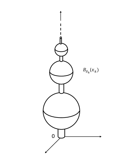
Figure 4: Example 7.4, Section 7

Let $v_{k}:B_{\delta_{k}}(x_{k})\to[0,1]$ be the function defined as

(7.13) $$v_{k}(x)=\big{(}1-\tfrac{|x-x_{k}|^{2}}{\delta_{k}^{2}}\big{)}^{i}\quad\hbox{for $x\in B_{\delta_{k}}(x_{k})$.}$$

We have that $\nabla^{\ell}v_{k}=0$ on $\partial B_{\delta_{k}}(x_{k})$ for $0\leq\ell\leq i-1$, and hence, given $\ell\leq i$ and $\varepsilon_{k}\in(0,\tfrac{\delta_{k}}{2})$, there exists a positive constant $c$ such that

(7.14) $$|\nabla^{\ell}v_{k}|\leq c{\delta_{k}}^{-i}\varepsilon_{k}^{i-\ell}$$

in an $\varepsilon$ neighborhood of $\partial B_{\delta_{k}}(x_{k})$. Moreover, if $\ell\leq 2i$, then there exists a positive constant $c$ such that

(7.15) $$|\nabla^{\ell}v_{k}|\geq c{\delta_{k}}^{-\ell}$$

in a subset of $B_{\delta_{k}}(x_{k})$ of Lebesgue measure $\approx{\delta_{k}}^{n}$, whereas, if $\ell>2i$, then

(7.16) $$\nabla^{\ell}v_{k}=0.$$

Next, denote by $y_{k}$ and $z_{k}$ the north and the south pole of $B_{\delta_{k}}(x_{k})$, respectively, and let $\rho:[0,\infty)\to[0,1]$ be a smooth function, which vanishes in $[0,\tfrac{1}{2}]$ and equals $1$ in $[1,\infty)$. Let us define the function $w_{k}:\Omega\to[0,\infty)$ as

(7.17) $$w_{k}(x)=v_{k}(x)\rho(|x-y_{k}|/\varepsilon_{k})\rho(|x-z_{k}|/\varepsilon_{k})\quad\hbox{for $x\in B_{\delta_{k}}(x_{k})$,}$$

and $w_{k}=0$ elsewhere, where $\varepsilon_{k}$ will be chosen later.
If $j\leq 2i$,

(7.18) $$|\nabla^{j}w_{k}|\geq c{\delta_{k}}^{-j}$$

in a subset of $B_{\delta_{k}}(x_{k})$ of Lebesgue measure $\approx{\delta_{k}}^{n}$, and, if $j>2i$,

(7.19) $$\nabla^{j}v_{k}=0\quad\hbox{in $B_{\delta_{k}}(x_{k})\setminus(B_{\varepsilon_{k}}(y_{k})\cup B_{\varepsilon_{k}}(z_{k}))$.}$$

Thus, there exists a constant $c$ such that

(7.20) $$|\nabla^{j}w_{k}|\leq c\sum_{\ell=0}^{\min\{j,2i\}}\varepsilon_{k}^{\ell-j}|\nabla^{\ell}v_{k}|\quad\hbox{in $B_{\varepsilon_{k}}(y_{k})\cup B_{\varepsilon_{k}}(z_{k})$.}$$

Consequently, if $j\leq m$, then

(7.21) $$|\nabla^{j}w_{k}|\leq c\varepsilon_{k}^{i-j}{\delta_{k}}^{-i}\quad\hbox{in $B_{\varepsilon_{k}}(y_{k})\cup B_{\varepsilon_{k}}(z_{k})$,}$$

for some constant $c$. Hence, if $j>2i$, then

(7.22) $$\|\nabla^{j}w_{k}\|_{L^{p}(B_{\delta_{k}}(x_{k}))}^{p}\leq c{\delta_{k}}^{-pi}\varepsilon_{k}^{p(i-j)+n}$$

for some constant $c$. On the other hand, if $j\leq 2i$, then

(7.23) $$\|\nabla^{j}w_{k}\|_{L^{p}(B_{\delta_{k}}(x_{k}))}^{p}\leq c\big{(}{\delta_{k}}^{n-pj}+{\delta_{k}}^{-pi}\varepsilon_{k}^{p(i-j)+n}\big{)}$$

for some constant $c$.

Set $\varepsilon_{k}=\delta_{k}^{\alpha}$, with $\alpha$ to be chosen later. Then, by (7.22) and (7.23),

(7.24) $$\|w_{k}\|_{V^{m,p}(B_{\delta_{k}}(x_{k}))}^{p} \leq c\big{(}{\delta_{k}}^{-pi+\alpha[p(i-m)+n]}+{\delta_{k}}^{n-2pi}+{\delta_{k}}^{-pi+\alpha(-pi+n)}\big{)}$$

$$\leq c\big{(}{\delta_{k}}^{-pi+\alpha[p(i-m)+n]}+{\delta_{k}}^{n-2pi}\big{)},$$

where the last inequality holds since $p(i-m)+n<-pi+n$, owing to the assumption that $i<\tfrac{m}{2}$.

Let us consider (7.11). Note that

(7.25) $$n>pi.$$

Indeed, since we are now assuming that $p(m-h)<n$ and $0\leq h\leq i<\tfrac{m}{2}$, we have that $n>p(m-h)\geq p(m-i)>p(2i-i)=pi$, namely (7.25).
We may choose $\alpha$ such that

(7.26) $$-pi+\alpha[p(i-m)+n]<n-2pi.$$

Actually, if $p(i-m)+n>0$, then inequality (7.26) holds provided that

(7.27) $$1<\alpha<\tfrac{n-pi}{p(i-m)+n}.$$

Note that the two inequalities in (7.27) are compatible since $i<\tfrac{m}{2}$. If, instead, $p(i-m)+n\leq 0$, then any choice of $\alpha>1$ is admissible, since $-pi+\alpha[p(i-m)+n]\leq-pi$, whence (7.26) follows, owing to (7.25).
By (7.24) and (7.26),

(7.28) $$\|w_{k}\|_{V^{m,p}(B_{\delta_{k}}(x_{k}))}^{p}\leq c{\delta_{k}}^{-pi+\alpha[p(i-m)+n]},$$

for some constant $c$. Given a sequence $\{\lambda_{k}\}$, define $w_{k}$ as

(7.29) $$u(x)=\sum_{k=1}^{\infty}\lambda_{k}w_{k}(x)\quad\hbox{for $x\in\Omega$.}$$

Note that $u=\nabla u=\dots=\nabla^{i-1}u=0$ on $\partial\Omega$.
Set $q=\frac{pn}{n-p(m-h)}$, and choose $\lambda_{k}=\delta_{k}^{h-\frac{n}{q}}$ for $k\in\mathbb{N}$. By (7.18), there exists a positive constant $c$ such that

(7.30) $$\|\nabla^{h}u\|_{L^{q}(\Omega)}^{q}=\sum_{k=1}^{\infty}\lambda_{k}^{q}\int_{B_{\delta_{k}}(x_{k})}|\nabla^{h}w_{k}|^{q}dx\geq c\sum_{k=1}^{\infty}\lambda_{k}^{q}\delta_{k}^{n-hq}=c\sum_{k=1}^{\infty}1=\infty.$$

On the other hand, by (7.28) there exists a constant $c$ such that

(7.31) $$\|u\|_{V^{m,p}(\Omega)}^{p}=\sum_{k=1}^{\infty}\lambda_{k}^{p}\|w_{k}\|_{V^{m,p}(B_{\delta_{k}}(x_{k}))}^{p}\leq c\sum_{k=1}^{\infty}\lambda_{k}^{p}\delta_{k}^{-pi+\alpha[p(i-m)+n]}=c\sum_{k=1}^{\infty}\delta_{k}^{(\alpha-1)[p(i-m)+n]}.$$

Our assumptions ensure that $p(i-m)+n\geq p(h-m)+n>0$. Thus, $(\alpha-1)[p(i-m)+n]>0$, and hence the last series in (7.31) converges, provided that $\delta_{k}$ decays to $0$ sufficiently fast. Clearly, equations (7.30) and (7.31) contradict (7.11).

Let us next focus on (7.12). Consider again the function $u$ given by (7.29). Fix $\sigma\in(0,h)$, and choose $\lambda_{k}=\delta_{k}^{h-\sigma}$. By (7.18),

(7.32) $$\|\nabla^{h}u\|_{L^{\infty}(\Omega)}\geq c\lim_{k\to\infty}\lambda_{k}\delta_{k}^{-h}=c\lim_{k\to\infty}\delta_{k}^{-\sigma}=\infty.$$

Moreover, by (7.24),

(7.33) $$\|u\|_{V^{m,p}(\Omega)}^{p}=\sum_{k=1}^{\infty}\lambda_{k}^{p}\|w_{k}\|_{V^{m,p}(B_{\delta_{k}}(x_{k}))}^{p} \leq c\sum_{k=1}^{\infty}\delta_{k}^{p(h-\sigma)}\big{(}\delta_{k}^{-pi+\alpha[p(i-m)+n]}+\delta_{k}^{n-2pi}\big{)}$$

$$=c\sum_{k=1}^{\infty}\big{(}\delta_{k}^{hp-\sigma p-pi+\alpha[p(i-m)+n]}+\delta_{k}^{hp-\sigma p+n-2pi}\big{)}.$$

The assumption $n>p\max\{m-i,2i-h\}$ ensures that

$$hp+n-2pi>0,\quad\hbox{and}\quad hp-pi+\alpha[p(i-m)+n]>0,$$

provided that $\alpha$ is sufficiently large. Since $\sigma$ can be chosen arbitrarily small, we may assume that both exponents of $\delta_{k}$ in the last series of (7.33) are positive, and hence that

(7.34) $$\|u\|_{V^{m,p}(\Omega)}<\infty,$$

provided that $\delta_{k}$ decays to $0$ fast enough. Equations (7.32) and (7.34) contradict (7.12).

Appendix

A result in the theory of Sobolev functions tells us that, if $u$ is any weakly differentiable function in ${{\mathbb{R}}^{n}}$, then

(7.35) $$|u(x)-u(y)|\leq C(M(|\nabla u|)(x)+M(|\nabla u|)(y))\quad\hbox{for a.e. $x,y\in{{\mathbb{R}}^{n}}$,}$$

for some constant $C$. Here, $M$ denotes the maximal function operator defined, for $f\in L^{1}_{\rm loc}({{\mathbb{R}}^{n}})$, as

$$Mf(x)=\sup_{B\ni x}\frac{1}{\mathcal{L}^{n}(B)}\int_{B}|f(y)|\,dy\qquad\hbox{for $x\in{{\mathbb{R}}^{n}}$,}$$

where $B$ denotes a ball in ${{\mathbb{R}}^{n}}$. Thus, $M(|\nabla u|)$ is an upper gradient for $u$ in the sense of metric measure spaces, as defined in [Ha].
The following proposition provides us with a higher-order counterpart of (7.35), and gives grounds for definitions (3.13) and (3.14).

Proposition 7.5

Let $n,\ell\in\mathbb{N}$. Then there exists a constant $C=C(\ell,n)$ such that, if $u\in W^{2\ell-1,1}_{\rm loc}({{\mathbb{R}}^{n}})$, then

(7.36) $$\left|\sum_{|\alpha|\leq\ell-1}\frac{(2\ell-2-|\alpha|)!}{(\ell-1-|\alpha|)!\alpha!}\frac{(y-x)^{\alpha}}{|y-x|^{2\ell-1}}\big{[}(-1)^{|\alpha|}D^{\alpha}u(y)-D^{\alpha}u(x)\big{]}\right|\\ \leq C\big{(}M(|\nabla^{2\ell-1}u|)(x)+M(|\nabla^{2\ell-1}u|)(y)\big{)}\quad\hbox{for a.e. $x,y\in{{\mathbb{R}}^{n}}$}.$$

Proof. By [Bo, Proposition 5.1], if $0\leq|\alpha|\leq 2\ell-2$, then there exists a measurable function $R_{2\ell-1,\alpha}(u):{{\mathbb{R}}^{n}}\times{{\mathbb{R}}^{n}}\to\mathbb{R}$ and a constant $C=C(\ell,n)$ such that

(7.37) $$D^{\alpha}u(y)=\sum_{|\gamma|\leq 2\ell-2-|\alpha|}\frac{(y-x)^{\gamma}}{\gamma!}D^{\alpha+\gamma}u(x)+R_{2\ell-1,\alpha}(u)(x,y)\quad\hbox{for a.e. $x,y\in{{\mathbb{R}}^{n}}$,}$$

and

(7.38) $$|R_{2\ell-1,\alpha}(u)(x,y)|\leq C|x-y|^{2\ell-1-|\alpha|}\big{[}M(|\nabla^{2\ell-1}u|)(x)+M(|\nabla^{2\ell-1}u|)(y)\big{]}\quad\hbox{for a.e. $x,y\in{{\mathbb{R}}^{n}}$}.$$

We claim that there exist constants $C(\alpha,\ell)$, for $|\alpha|\leq\ell-1$, such that

(7.39) $$\sum_{|\alpha|\leq\ell-1}\frac{(2\ell-2-|\alpha|)!}{(\ell-1-|\alpha|)!\alpha!}\frac{(y-x)^{\alpha}[D^{\alpha}u(x)+(-1)^{|\alpha|+1}D^{\alpha}u(y)]}{|y-x|^{2\ell-1}}\\ =\sum_{|\alpha|\leq\ell-1}\frac{C(\alpha,\ell)(y-x)^{\alpha}}{|y-x|^{2\ell-1}}R_{2\ell-1,\alpha}(u)(x,y)\quad\hbox{for a.e. $x,y\in{{\mathbb{R}}^{n}}$}.$$

Inequality (7.36) will then follow from (7.39) and (7.38).
Let us establish (7.39). By (7.37), after exchanging the order of summation and relabeling the indices, one obtains that there exist constants $A(\alpha,\ell)$ and $B(\alpha,\ell)$, for $|\alpha|\leq\ell-1$, such that

(7.40) $$\sum_{|\alpha|\leq\ell-1} \frac{(2\ell-2-|\alpha|)!}{(\ell-1-|\alpha|)!\alpha!}(y-x)^{\alpha}\frac{[D^{\alpha}u(x)+(-1)^{|\alpha|+1}D^{\alpha}u(y)]}{|y-x|^{2\ell-1}}$$

$$=\sum_{|\alpha|\leq\ell-1}\frac{(2\ell-2-|\alpha|)!}{(\ell-1-|\alpha|)!\alpha!}\frac{(y-x)^{\alpha}}{|y-x|^{2\ell-1}}$$

$$\times\bigg{[}D^{\alpha}u(x)+(-1)^{|\alpha|+1}\bigg{(}\sum_{|\gamma|\leq 2\ell-2-|\alpha|}\frac{(y-x)^{\gamma}}{\gamma!}D^{\alpha+\gamma}u(x)+R_{2\ell-1,\alpha}(u)(x,y)\bigg{)}\bigg{]}$$

$$=\sum_{|\alpha|\leq 2\ell-2}\frac{(y-x)^{\alpha}}{|y-x|^{2\ell-1}}A(\alpha,\ell)D^{\alpha}(u)(x)+\sum_{|\alpha|\leq\ell-1}\frac{(y-x)^{\alpha}}{|y-x|^{2\ell-1}}B(\alpha,\ell)R_{2\ell-1,\alpha}(u)(x,y)$$

for a.e. $x,y\in{{\mathbb{R}}^{n}}$.
Now, let us choose $u=\mathcal{P}$ in (7.40), where $\mathcal{P}$ is a polynomial of the form

(7.41) $$\mathcal{P}(y)=\sum_{|\alpha|\leq 2\ell-2}b_{\alpha}(y-x)^{\alpha}\quad\hbox{for $y\in{{\mathbb{R}}^{n}}$,}$$

with $b_{\alpha}\in\mathbb{R}$. Clearly,

(7.42) $$D^{\alpha}\mathcal{P}(x)=\alpha!b_{\alpha} |\alpha|\leq 2\ell-2 D^{\alpha}\mathcal{P}(x)=0 |\alpha|>2\ell-2$$ if ,    if .

Hence, $R_{2\ell-1,\alpha}(\mathcal{P})(x,y)=0$, and from (7.40) we obtain that

(7.43) $$\sum_{|\alpha|\leq\ell-1}\frac{(2\ell-2-|\alpha|)!}{(\ell-1-|\alpha|)!\alpha!}(y-x)^{\alpha}\frac{[D^{\alpha}\mathcal{P}(x)+(-1)^{|\alpha|+1}D^{\alpha}\mathcal{P}(y)]}{|y-x|^{2\ell-1}}=\sum_{|\alpha|\leq 2\ell-2}\frac{(y-x)^{\alpha}}{|y-x|^{2\ell-1}}A(\alpha,\ell)\alpha!b_{\alpha}$$

for a.e. $x,y\in{{\mathbb{R}}^{n}}$. We next express the leftmost side of (7.40) in an alternative form. Define $\varphi:\mathbb{R}\to\mathbb{R}$ as

$$\varphi(t)=u(x+t\vartheta)\quad\hbox{for $t\in\mathbb{R}$,}$$

where

$$\vartheta=\frac{y-x}{|y-x|}.$$

Given $j\in\{1,\dots,2\ell-1\}$, we have that

(7.44) $$\varphi^{(j)}(t) =\sum_{|\alpha|=j}\frac{j!}{\alpha!}\vartheta^{\alpha}D^{\alpha}u(x+t\vartheta)\quad\hbox{for a.e. $t\in\mathbb{R}$.}$$

Thus, by the Taylor formula centered at $t=0$, if $k\in\{1,\dots,2\ell-1\}$, then

(7.45) $$\varphi^{(k)}(|y-x|) =\sum_{j=k}^{2\ell-2}\frac{\varphi^{(j)}(0)}{(j-k)!}|y-x|^{j-k}+Q_{2\ell-1,k}(\varphi)(|y-x|)$$

$$=\sum_{j=k}^{2\ell-2}\frac{1}{(j-k)!}\sum_{|\alpha|=j}\frac{j!}{\alpha!}|y-x|^{j-k}\vartheta^{\alpha}D^{\alpha}u(x)+Q_{2\ell-1,k}(\varphi)(|y-x|)$$

for a.e. $x,y\in{{\mathbb{R}}^{n}}$, where $Q_{2\ell-1,k}(\varphi)$ denotes the remainder in the $(2\ell-2-k)$-th order Taylor formula for $\varphi^{(k)}$, centered at $t=0$. By (7.44) and (7.45), there exist constants $A^{\prime}(\alpha,\ell)$ and $B^{\prime}(\alpha,\ell)$ such that

(7.46) $$\sum_{|\alpha|\leq\ell-1}\frac{(2\ell-2-|\alpha|)!}{(\ell-1-|\alpha|)!\alpha!}(y-x)^{\alpha}\frac{[D^{\alpha}u(x)+(-1)^{|\alpha|+1}D^{\alpha}u(y)]}{|y-x|^{2\ell-1}}$$

$$=(-1)^{\ell}\sum_{k=0}^{\ell-1}\frac{(2\ell-k-2)!}{k!(\ell-k-1)!}\frac{\big{[}\varphi^{(k)}(0)+(-1)^{k+1}\varphi^{(k)}(|y-x|)\big{]}}{|y-x|^{2\ell-k-1}}$$

$$=(-1)^{\ell}\sum_{k=0}^{\ell-1}\frac{(2\ell-k-2)!}{k!(\ell-k-1)!}\frac{1}{|y-x|^{2\ell-k-1}}$$

$$\times\bigg{[}\sum_{|\alpha|=k}\frac{k!}{\alpha!}\vartheta^{\alpha}D^{\alpha}u(x)+(-1)^{k+1}\bigg{(}\sum_{j=k}^{2\ell-2}\frac{1}{(j-k)!}|y-x|^{j-k}\sum_{|\alpha|=j}\frac{j!}{\alpha!}\vartheta^{\alpha}D^{\alpha}u(x)+Q_{2\ell-1,k}(\varphi)(|y-x|)\bigg{)}\bigg{]}$$

$$=\sum_{|\alpha|\leq 2\ell-2}\frac{(y-x)^{\alpha}}{|y-x|^{2\ell-1}}A^{\prime}(\alpha,\ell)D^{\alpha}u(x)+\sum_{|\alpha|\leq\ell-1}\frac{1}{|y-x|^{2\ell-|\alpha|-1}}B^{\prime}(\alpha,\ell)Q_{2\ell-1,|\alpha|}(\varphi)(|x-y|)$$

for a.e. $x,y\in{{\mathbb{R}}^{n}}$. If $\mathcal{P}$ is again a polynomial in $t$ of the form (7.41), then $\varphi$ is also a polynomial of degree not exceeding $2\ell-2$ , and from (7.42) and (7.46), applied with $u=\mathcal{P}$, we obtain that

(7.47) $$\sum_{|\alpha|\leq\ell-1}\frac{(2\ell-2-|\alpha|)!}{(\ell-1-|\alpha|)!\alpha!}(y-x)^{\alpha}\frac{[D^{\alpha}\mathcal{P}(x)+(-1)^{|\alpha|+1}D^{\alpha}\mathcal{P}(y)]}{|y-x|^{2\ell-1}}=\sum_{|\alpha|\leq 2\ell-2}\frac{(y-x)^{\alpha}}{|y-x|^{2\ell-1}}A^{\prime}(\alpha,\ell)\alpha!b_{\alpha}$$

for a.e. $x,y\in{{\mathbb{R}}^{n}}$. Owing to the arbitrariness of the coefficients $b_{\alpha}$, we infer from (7.43) and (7.47) that

(7.48) $$A(\alpha,\ell)=A^{\prime}(\alpha,\ell)$$

for every multi-index $\alpha$ such that $|\alpha|\leq 2\ell-2$. On the other hand, by (4.23) and (4.24), applied with $\varsigma=\psi=\varphi$, $a=0$ and $b=|y-x|$, and by (7.46) and (7.47),

(7.49) $$0 =\varphi^{(2\ell-1)}(t)=\bigg{[}\frac{d^{\ell-1}}{dt^{\ell-1}}\bigg{(}\frac{\varphi(t)}{(t-|y-x|)^{\ell}}\bigg{)}_{|t=0}+\frac{d^{\ell-1}}{dt^{\ell-1}}\bigg{(}\frac{\varphi(t)}{t^{\ell}}\bigg{)}_{|t=|y-x|}\bigg{]}$$

$$=(-1)^{\ell}\sum_{k=0}^{\ell-1}\frac{(2\ell-k-2)!}{k!(\ell-k-1)!}\frac{\big{[}\varphi^{(k)}(0)+(-1)^{k+1}\varphi^{(k)}(|y-x|)\big{]}}{|y-x|^{2\ell-k-1}}$$

$$=\sum_{|\alpha|\leq\ell-1}\frac{(2\ell-2-|\alpha|)!}{(\ell-1-|\alpha|)!\alpha!}\frac{(y-x)^{\alpha}[(-1)^{|\alpha|+1}D^{\alpha}u(y)+D^{\alpha}u(x)]}{|y-x|^{2\ell-1}}$$

$$=\sum_{|\alpha|\leq 2\ell-2}\frac{(y-x)^{\alpha}}{|y-x|^{2\ell-1}}A^{\prime}(\alpha,\ell)\alpha!b_{\alpha}$$

for a.e. $x,y\in{{\mathbb{R}}^{n}}$. By the arbitrariness of the coefficients $b_{\alpha}$ again, $A^{\prime}(\alpha,\ell)=0$ for every $\alpha$ such that $|\alpha|\leq 2\ell-2$. Hence, owing to (7.48),

(7.50) $$A(\alpha,\ell)=0$$

for every $\alpha$ such that $|\alpha|\leq 2\ell-2$. Equations (7.40) and (7.50) tell us that

(7.51) $$\sum_{|\alpha|\leq\ell-1} \frac{(2\ell-2-|\alpha|)!}{(\ell-1-|\alpha|)!\alpha!}(y-x)^{\alpha}\frac{D^{\alpha}u(x)+(-1)^{|\alpha|+1}D^{\alpha}u(y)]}{|y-x|^{2\ell-1}}$$

$$=\sum_{|\alpha|\leq\ell-1}\frac{(y-x)^{\alpha}}{|y-x|^{2\ell-1}}B(\alpha,\ell)R_{2\ell-1,\alpha}(u)(x,y)\quad\hbox{for a.e. $x,y\in{{\mathbb{R}}^{n}}$,}$$

whence (7.39) follows with $C(\alpha,\ell)=B(\alpha,\ell)$.