Distinct nodes visited by random walkers on scale-free networks

Abstract

Random walks on discrete lattices are fundamental models that form the basis for our understanding of transport and diffusion processes. For a single random walker on complex networks, many properties such as the mean first passage time and cover time are known. However, many recent applications such as search engines and recommender systems involve multiple random walkers on complex networks. In this work, based on numerical simulations, we show that the fraction of nodes of scale-free network not visited by $W$ random walkers in time $t$ has a stretched exponential form independent of the details of the network and number of walkers. This leads to a power-law relation between nodes not visited by $W$ walkers and by one walker within time $t$. The problem of finding the distinct nodes visited by $W$ walkers, effectively, can be reduced to that of a single walker. The robustness of the results is demonstrated by verifying them on four different real-world networks that approximately display scale-free structure.

Random walks were introduced more than a century ago and have formed the basis for our understanding of diffusion processes in physical systems (rw, ). As a fundamental stochastic process, they are relevant for many fields ranging from physics and computer sciences (web, ) to biology (rwbio, ) and economics (eco, ). Several problems including animal foraging and migration (forag, ; migr, ), emergence of innovation inno , intracellular molecular transport insulin , proteins binding with DNA sequences dna1 , for structual information about macromolecules bio are based on the dynamics of a single random walker on regular lattice or its variants.

On the other hand, many recent applications involve dynamics of multiple random walkers on a disordered lattice, e.g., complex network with non-local edges connecting the nodes. For instance, cellular signal transduction (cell, ), exciton transport in molecular crystals, web search algorithms (web, ), a class of image segmentation algorithms imseg , graph clustering gclust and recommender systems (llu, ) widely used for personalization in popular websites are based on the idea of many random walkers exploring a topology of discrete nodes connected through their edges.

As a statistical physics problem, in comparison to the well-studied problem of the dynamics of a single random walker on regular lattice mont or complex network porter ; burioni , the case of multiple walkers in a network setting has not attracted sufficient research attention. In random walk with $W$ non-interacting walkers, some results are a straightforward generalisation of that for single walker dynamics. For instance, on a complex network, occupation probability of a single walker on a node with degree $k$ is proportional to $k$, whereas for $W$ walkers it is $\propto Wk$. However, in many cases, the results for multiple walker dynamics is not a trivial generalization of that for a single walker. One such statistical quantity of interest is the mean number of distinct sites $S_{W}(t)$ visited by $W$ random walkers in $t$ discrete time steps on a network with $N$ nodes. This is relevant for problems related to (mis-)information and contagion spreading and search problems on networks (epi, ).

Distinct sites visited in $t$-steps by a random walker was studied in Refs. (de, ) and its generalization to $W$ walkers was considered in Refs. (stan, ; weiss, ). On regular $d$-dimensional lattices and for short times, the mean number of distinct sites visited by $W$ walkers is $\langle S_{W}(t)\rangle\propto t^{d}$ and asymptotically $\langle S_{W}(t)\rangle\propto Wt$ for $d>3$. In general, Ref. (stan, ) identifies three distinct time scales with different behaviours for $\langle S_{W}(t)\rangle$ and limited analytical support is presented in Ref. (yuste, ). Recently, an exact asymptotic result for the distribution of number of distinct and common sites visited by $W$ walkers on a regular 1$d$ lattice was obtained (snm1, ) by transforming it as a problem of extreme value statistics.

In spite of these developments for regular lattices, very few results are known for multiple random walkers on complex networks. For a random walker on a Bethe lattice with coordination number $z$, $S_{1}(t)=((z-2)/(z-1))t$, for $z\geq 3$ (bethe, ). Clearly, $S_{1}(t)\propto n$ with a prefactor that depends on the local topology of the lattice. On a random network, a formal relation for the generating function corresponding to $S_{1}(t)$ has been obtained in terms of the generating functions for the first passage probabilities (snm2, ). For a walker on scale-free network, it was numerically shown that, for short times, $S_{1}(t)=t$ and as $t\to\infty,S_{1}(t)\to 1$ due to finite size of network (slee, ). On a small world network, $S_{1}(t)$ displays a cross-over from $\sqrt{t}$ to linear behaviour depending on whether the walker has managed to hit a short-cut in the small world network or not (kulk, ).

To the best of our knowledge, exact closed form result for $\langle S_{W}(t)\rangle$ on an arbitrary network with $N$ nodes is not yet known. Even as this gap continues to exist, in this work, new results primarily based on numerical simulations are presented that effectively relate $S_{W}(t)$ to $S_{1}(t)$ on static networks. In particular, for the class of scale-free networks, it is shown that the number of nodes $s_{W}(t)$ not yet visited until time $t$ has a stretched exponential form, with exponent $\beta$, depending on the specific network structure but independent of the number of walkers. As shown below, the results are consistent with $s_{W}(t)\propto\exp(W^{\beta}s_{1}(t))$. Thus, effectively, the problem of finding $S_{W}(t)$ can be reduced to a relatively simpler problem of finding $S_{1}(t)$ on a scale-free network.

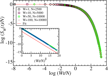
(a)

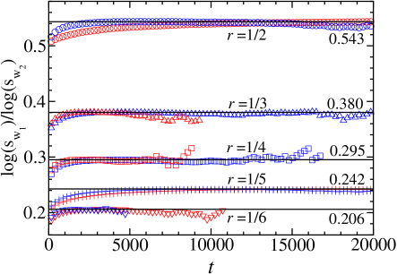
(b)

Figure 1: (a) Fraction of nodes not reachable by random walkers on Barabasi-Albert scale-free network plotted as a function of $x=Wt/N$. Symbols are from random walk simulations and were averaged over 1000 realizations. The solid (red) curve is the best fit line. Note the excellent scaling collapse. (Inset) shows the same data (in semi-log scale) as a function of $(Wt/N)^{\beta}$. The best fit (solid) line with slope $\beta=0.693$ is given a vertical offset for easier comparison with simulation data. (b) The ratio $u(t)$ shown as a function of $t$. Validity of scaling can be inferred from the flat lines obtained from simulations. In this, $r=W_{1}/W_{2}$ and the value of $r^{\beta}$ is also indicated.

Distinct sites visited by multiple walkers $S_{W}(t)$ can also be thought of as a statistical relaxation process especially if the initial position of the walkers is far from equilibrium distribution. On a network, this is easily achieved by placing all the walkers on the same node at $t=0$. In this garb, $s_{W}(t)=N(1-S_{W}(t)/N)$ represents a relaxation process and the results presented here indicate scaling of this process as a function of $W$ and $N$. Such relaxation processes in a wide variety of disordered condensed matter systems is known to display a stretched exponential decay of auto-correlations of the form $C(t)=\exp(-t/\tau)^{\beta}$, where $\tau$ is a parameter with dimensions of inverse time and $0\leq\beta\leq 1$ is the exponent (klafter, ). The results obtained in this work add to the list of known systems that display stretched exponential relaxation. If $S_{W}(t)$ denotes the unique ’territory’ covered by $W$ walkers, then $s_{W}(t)$ represents its complementary part, the territory unreachable in time $t$. Thus $s_{W}(t)+S_{W}(t)=1$ for all $t$ and we have chosen to present results for $s_{W}(t)$ in the rest of the paper.

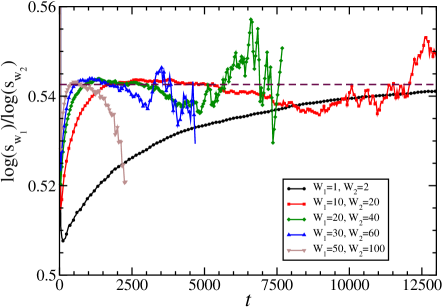
Figure 2: The ratio $u(t)$ shown as a function of $t$ for several choices of $W_{1}$ and $W_{2}$. The deviations from the scaling relation in Eq. 2 arise due to finite number of walkers and finite size of the network. See text for a detailed explanation. This simulations were performed on Barabasi-Albert scale-free network with $N=10000$ nodes (same as one of the networks used in Fig. 1(a)).

Random walks on complex networks are a straightforward generalisation of random walks on regular lattices. In this work, independent and multiple walkers randomly walk on a connected, scale-free network with $N$ nodes and $E$ edges generated using Barabasi-Albert (BA) (scale, ) and configuration models (newman, ). Each node has an associated degree $k_{i},i=1,2...N$, indicating the number of edges. The degree distribution of the network is $P(k)\sim k^{-\gamma}$, where $\gamma$ is the exponent. A walker at $i$-th node can hop to any of its connected neighbours with probability $1/k_{i}$. The information on the edges in the network are encoded in the adjacency matrix ${\mathbf{A}}$ of order $N$, where the element $A_{ij}=1$ if nodes $i$ and $j$ are connected by an edge, and $A_{ij}=0$ if they are not connected.

In Fig. 1(a), the fraction of nodes not reached in time $t$, $s_{W}(t)$, is shown for BA scale-free networks ${\mathcal{N}}_{BA}(N,E,\gamma)$. Each data point is averaged over 1000 random walk realizations. At time $t=0$, all the $W$ walkers are all placed on a randomly chosen node designated as zeroth node, i.e., $w_{0}(t=0)=\sum_{i}W\delta_{i,0}$. This figure shows results for four different values of $N$ and $W$. Remarkably, in all the cases, the scaled parameter can be identified as $x=Wt/N$. With this choice, scaling is evident from the excellent data collapse observed in Fig. 1(a). It can be inferred (from the fitted solid line) that as $W\to\infty$ and $N\to\infty$, the fraction of unreachable nodes is consistent with a stretched exponential function of the form,

$$s_{W}(t)=\left(\frac{N-1}{N}\right)~{}e^{-A~{}x(t)^{\beta}},$$ (1)

in which the parameters $A$ and $\beta$ are estimated through a regression procedure. For the simulations shown in Fig. 1, $A\approx 0.75$ and $\beta\approx 0.88$. The scaled time $x=Wt/N$ can also be expressed in units of mean relaxation time as $x=C_{\beta}~{}t/\tau_{r}$, where $\tau_{r}=C_{\beta}N/W$ and $C_{\beta}=\frac{A~{}\Gamma(2/\beta)}{\beta~{}\Gamma(1+1/\beta)}$. For single walker dynamics, $W=1$ and scaled time reduces to $x=t/N$, in agreement with the results in Ref. (slee, ). The inset in Fig. 1(a) displays the same data as in the main figure as a function of $x^{\beta}$ and its linearity suggests Eq. 1. For $x\ll 1$, Eq. 1 becomes $s_{W}(t)\approx 1-Ax^{\beta}$. Thus, the fraction of distinct sites visited is $S_{W}(t)\approx Ax^{\beta}$.

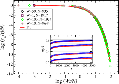
Figure 3: Fraction of nodes not reachable by random walkers on configuration model of scale-free networks plotted as a function of $x=Wt/N$. Symbols are obtained from random walk simulations averaged over 1000 realizations. The solid (red) line represents Eq. 1 with $A=0.601$ and $\beta=0.653$ obtained through regression. Note the excellent scaling collapse. (Inset) demonstrates the scaling of $s_{w}(t)$ (Eq. 2) for different number of walkers $w_{1}$ and $w_{2}$. The solid (horizontal) lines are the expected value, namely, $(W_{2}/W_{1})^{\beta}$ for $W_{2}/W_{1}$ ratios $1/2$, $2/5$, $1/3$ and $1/4$.

In connected and finite size networks, unreachable nodes is a finite time effect since as $t\to\infty$ all the nodes are eventually reached. Then, we can expect the scaling relation in Eq. 1 to hold good in the timescale $\tau_{r}<t\ll t_{cov}$, where $t_{cov}$ is the cover time for all the nodes to be visited at least once. For a single walker on a scale-free network, $t_{cov}\leq N\log N$, though a similar result for multiple walkers is not yet known (alon, ). Since multiple walkers are known to improve efficiency of covering network (alon, ), in this case, $N\log N$ will essentially be a loose upper bound.

Based on Eq. 1, the central result of this paper can be recast in the form of a scaling relation as $N\to\infty$, $W_{1},W_{2}\to\infty$ and it is of the form

$$\log s_{W_{2}}(t)=\left(\frac{W_{2}}{W_{1}}\right)^{\beta}~{}\log s_{W_{1}}(t).$$ (2)

This is valid for $W_{1},W_{2}\gg 0$ random walkers on a given scale-free network ${\mathcal{N}}_{s}(N,E,\gamma)$. Remarkably, the relation between $s_{W_{1}}$ and $s_{W_{2}}$ depends only on the ratio $r=W_{1}/W_{2}$ and information about network enters through the exponent $\beta$. This is verified in Figure 1(b) by plotting the ratio $u(t)=\log s_{W_{1}}(t)/\log s_{W_{1}}(t)$ as a function of time $t$. In this form, presence of scaling is inferred from horizontal lines such that $u(t)=\phi=r^{\beta}$, a constant. In particular, simulations confirm that $\phi$ is identical for any choice of $W_{1}$ and $W_{2}$ such that $r$ is a constant.

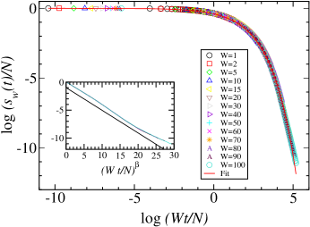
(a)

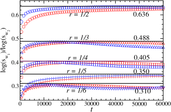
(b)

Figure 4: (a) For Enron email network, the fraction of nodes not reached by random walkers $s_{W}(t)$ as a function of scaled parameter $x$ (in log-log scale) for several values of $W$. The data collapse points to an agreement with Eq. 1 with $A=0.403$ and $\beta=0.652$. (Inset) shows that the same data becomes linear in semi-log plot if plotted as a function of $(Wt/N)^{\beta}$. (b) Demonstrates of the scaling relation in Eq. 2 for various choices of $r=W_{1}/W_{2}$.

The deviations observed in Fig. 1(b) in the vicinity of $t=0$ arise due to the finite number of walkers on the network. As shown in Fig. 2, as $W\to\infty$ the agreement with the scaling curve in Eq. 2 gets better. On the other hand, the deviations observed in Fig. 1(b) for $t>>1$ arise due to the finite size of the network. In finite size networks, as $t\to\infty$ nearly all the nodes are ultimately reached and hence there is no further ’territory’ to be explored leading to deviations from Eq. 1. Notice also that if the agreement with scaling relation is reached faster, as in the case of $W_{1}=50,W_{2}=100$ in Fig. 2, the deviations for $t>>1$ also happen earlier in comparison with the case of, say, $W_{1}=20$ and $W_{2}=40$. Physically, this happens because more the number of walkers, agreement with scaling curve is reached faster and the all the nodes are visited quickly (than for smaller number of walkers), and hence the deviation for $t>>1$ also appears quickly.

In Fig. 3, $s_{w}(t)$ is shown for a scale-free network obtained from the configuration model. For this case too, scaled time $x(t)=Wt/N$ leads to an excellent data collapse and Eq. 1 fits the data. The parameters $A=0.1$ and $\beta=0.2$ were estimated through regression. The inset in Fig. 3 shows the validity of the scaling relation in Eq. 2 for the random walks on configuration model for several choices of $W_{1}$ and $W_{2}$.

Network	A	$\beta$
Barabsi-Albert	0.724	0.882
Model
Configuration Model ($\gamma=2.2$)	0.601	0.653
Enron Email Network	0.403	0.652
Yeast Network	0.564	0.622
Autonomous Systems	0.601	0.712
Scientific Collaboration	0.273	0.582
Network

Table 1: The values of $A$ and $\beta$ in Eq. 1 obtained through regression for various scale-free network models.

Next, we study the distinct sites visited by random walkers on four real-life networks, namely, (a) the Enron email (EE) network and (b) protein-protein interaction network of a yeast, (c) network of autonomous systems of the Internet connected with each other from the CAIDA project and (d) scientific collaboration network of cond-mat papers. We perform simulation of random walks on these networks with $W$ walkers and the results are presented in Figs. 4-6. The data sets for (a,c,d) are obtained from Stanford network database snap and for (b) is obtained from Pajek database pajek . All these networks were extensively studied for their topological properties and, in particular, their degree distribution is known to display a power-law form, $P(k)\sim k^{-\gamma}$. For Enron email network $\gamma\approx 1.76$ koblenz , for yeast network $\gamma\approx 2.5$ albert , for network of autonomous systems $\gamma\approx 2.09$ koblenz and for the network of cond-mat papers $\gamma\approx 2.81$ koblenz . For the purposes of this work, the largest connected component of these networks was considered to ensure that isolated nodes do not exist.

Figure 4(a) shows random walk simulation results for the fraction of nodes not visited until time $t$ on the Enron email communication network. Random walk simulations were performed with different number of walkers $W$. As this figure reveals, the simulation results are in good agreement with the postulated relation in Eq. 1, with $A\approx 0.403$ and $\beta\approx 0.652$. In this case as well, $x=Wt/N$ is the scaled time and as seen in Fig. 4(a), an excellent data collapse is observed for number of walkers ranging from 1 to 100. The inset in Fig. 4(a) shows the same data as a function of $(Wt/N)^{\beta}$ and the resulting straight line supports Eq. 1. Further, Fig. 4(b) shows the validity of scaling relation in Eq.2 for various ratio of walkers $r=W_{1}/W_{2}$. In Fig. 5(a), $s_{W}(t)$ is shown as a function of scaled parameter for various choices of of $W$ in log-log scale. As expected, an excellent data collapse is observed in agreement with Eq. 1. The inset to this figure further confirms the temporal decay of $s_{W}(t)$ is indeed stretched exponential in form. As would be expected, a good agreement with scaling relation in Eq. 2 is seen in Fig. 5(b) for various ratio of walkers $r=W_{1}/W_{2}$.

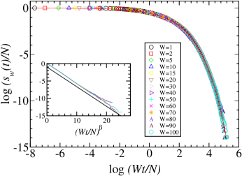
(a)

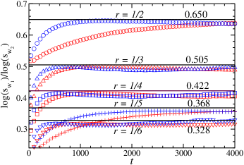
(b)

Figure 5: (a) Fraction of nodes not reached by $W$ random walkers in the network of protein-protein interaction in yeast. The decay follows Eq. 1 with $A=0.534$ and $\beta=0.635$. (b) The number of nodes not reached by $W_{1}$ and $W_{2}$ walkers follows the scaling relation in Eq. 2.

The scaling results from random walker simulations on a network of autonomous systems and author collaboration networks from cond-mat are displayed in Fig. 6. In these cases too, the simulation results for $s_{w}(t)$ display an excellent data collapse when plotted as a function of $x$ (not shown here). The values of parameters $A$ and $\beta$ estimated through regression is summarised in Table 1 for all the networks, including the ones corresponding to Fig. 6, discussed in this work. A good agreement with the scaling form in Eq. 2 is shown in Fig. 6. For $t>\tau_{r}$, the ratio $\log(s_{w_{1}})/\log(s_{w_{2}})$ tends to a constant dependent on the value of $\beta$, $W_{1}$ and $W_{2}$.

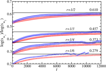
(a)

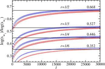
(b)

Figure 6: The ratio $u(t)$ as a function of time for random walk simulations performed on (a) a network of autonomous systems and (b) the scientific collaboration network of papers in cond-mat. In (a) and (b), the value of $(W_{1},W_{2})$ for each red curve is (5,10) for circles, (5,15) for up-triangles, (5,20) for squares, (5,30) for plus symbols. Corresponding values for blue curves are (10,20), (10,30), (10,40) and (10,60) respectively. The horizontal black lines correspond to $(W_{1}/W_{2})^{\beta}$. In all the cases, numerical random walk simulations tends to this constant after the relaxation time $\tau_{r}$.

In summary, we have studied the problem of distinct number of sites visited by multiple walkers on a scale-free network. Through numerical simulations, we have shown that the mean number of sites not reached until time $t$ can be represented by a stretched exponential function in Eq. 1 with $x=Wt/N$ being the scaled parameter. Using this, we have displayed the results in the form of a scaling relation (Eq. 2) between the nodes not reached in time $t$ by $W_{1}$ and $W_{2}$ walkers on the same network. Thus, effectively, the problem of finding the distinct sites visited by $W$ walkers on scale-free networks is related to that of one walker, effectively simplifying the problem. Thus, for scale-free networks, exact results for $s_{w}(t)$ for one walker would also help solve the problem for many walkers. This results gets better as the size of the network $N$ and number of walkers $W$ tend to larger values. We have numerically demonstrated these results for random walk dynamics on Barabasi-Albert scale-free network and that constructed using configuration model. Finally, we verified all our results by simulating random walks on four different real world scale-free networks and showing that the scaling holds. It turns out that the scale-free network is somewhat special as far as this scaling relations are concerned because we did not observe such scaling relations for the other popular classes of networks, namely, small-world and Erdos-Renyi random networks.

While the stretched exponential function is ubiquitous in the study of relaxation processes in condensed matter systems klafter , there are very few models in which stretched exponential decay of some observable occurs naturally. We propose that this simple model of random walks on scale-free networks with unreachability as the observable can be used as a model to investigate relaxation dynamics. We have seen that the stretching exponent $\beta$ varies, though not systematically, for different values of the power law exponent $\gamma$ of the degree distribution of the scale-free networks. This shows that $\beta$ has a dependence on the finer details of the structure of the network. An interesting and promising direction would be obtain analytical justifications for the scaling relation reported in this work.

- (1) S. Chandrasekhar, Rev. Mod. Phys. 15, 1 (1943); J. Rudnik and G. Gaspari, Elements of the random walk : An introduction for advanced students and researchers, (Cambridge University Press, 2004); Barry D. Hughes, Random walks and random environments, volume 1, (Clarendon Press, 1995).
- (2) F. R. K. Chung and W. Zhao, Bolyai Soc. Math. Stud. 20, 43 (2010).
- (3) E. A. Codling, M. J. Plank, and S. Benhamou, J. R. Soc. Interface 5, 813 (2008).
- (4) Eugene F. Fama, American Economic Review 104, 1467 (2014).
- (5) G. M. Viswanathan, M. G. E. da Luz, E. P. Raposo and H. E. Stanley, The Physics of Foraging, (Cambridge University Press, New York, 2011).
- (6) G. M. Viswanathan, E. P. Raposo and M. G. E. da Luz, Physics of Life Reviews 5, 133 (2008); G. M. Viswanathan, et. al., Nature 381, 413 (1996).
- (7) I. Iacopini, S. Milojevic and V. Latora, Phys. Rev. Lett. 120, 048301 (2018).
- (8) S. M. Ali Tabei et. al., PNAS 110, 4911 (2013).
- (9) L. Mirny et. al., J. Phys. A : Math. Theor. 42, 434013 (2009); C. Loverdo et. al., Phys. Rev. Lett. 102, 188101 (2009).
- (10) R. Phillips, J. Kondev, J. Theriot, and H. Garcia, Physical Biology of the Cell, (Garland Science, New York, 2013).
- (11) T. Lu, T. Shen, C. Zong, J. Hasty and P. G. Wolynes, PNAS 103, 16752 (2006).
- (12) L. Grady, IEEE Trans. on Pattern Analysis and Machine Intelligence 28, 1768 (2006).
- (13) S. A. Tabrizi, A. Shakery, M. Azadpour, M. Abbasi and M. A. Tavallaie, Physica A 392, 5772 (2013).
- (14) L. Lü et. al., Phys. Rep. 519, 1 (2012).
- (15) E. W. Montroll and G. H. Weiss, J. Math. Phys. 6, 167 (1965); J. W. Haus and K. W. Kehr, Phys. Rep. 150, 263 (1987).
- (16) N. Masuda, M. A. Porter, R. Lambiotte, Phys. Rep 716, 1 (2017).
- (17) R. Burioni and D.Cassi, J. Phys. A : Math. Gen. 38, R45 (2005).
- (18) M. Draief and L. Massouli, Epidemics and Rumours in Complex Networks, (Cambridge University Press, New York, 2010).
- (19) A. Dvoretzky and P. Erdos, in Proceedings of the Second Berkeley Symposium on Mathematical Statistics and Probability, (University of California, Berkeley, 1951).
- (20) H. Larralde, P. Trunfio, S. Havlin, H. E. Stanley, and G. H. Weiss, Phys. Rev. A 45, 7128 (1992); ibid, Nature 355, 423 (1992).
- (21) G. H. Weiss et. al., Physica A 191, 479 (1992).
- (22) S. B. Yuste and L. Acedo, Phys. Rev. E 61, 2340 (2000).
- (23) A. Kundu, S. N. Majumdar, and G. Schehr, Phys. Rev. Lett. 110, 220602 (2013).
- (24) B. D. Hughes and M. Sahimi, J. Stat. Phys. 29, 781 (1982).
- (25) C. De Bacco, S. N. Majumdar, and P. Sollich, J. Phys. A 48, 205004 (2015).
- (26) S. Lee, Soon-Hyung Yook and Y. Kim, Physica A 387, 3033 (2008).
- (27) E. Almaas, R. V. Kulkarni, and D. Stroud, Phys. Rev. E 68, 056105 (2003).
- (28) J. Klafter and M. F. Schlesinger, PNAS 83, 848 (1986).
- (29) R. Albert and A. L. Barabási, Rev. Mod. Phys. 74, 47 (2002).
- (30) M. E. J. Newman, in Handbook of Graphs and Networks : From the Genome to the Internet, (Wiley-VCH, Berlin, 2003).
- (31) N. Alon et. al., arXiv:0705.0467
- (32) B. F. Maier and D. Brockmann, Phys. Rev. E 96, 042307 (2017).
- (33) J. Leskovec and A. Krevl, SNAP Dataset at http://snap.stanford.edu/data (2014).
- (34) V. Batagelj and A. Mrvar, Pajek dataset at http://vlado.fmf.uni-lj.si/pub/networks/data/ (2006).
- (35) This value provided in http://konect.uni-koblenz.de/test/networks/
- (36) R. Albert, J. Cell Sci. 118, 4947 (2005).