Nonlinear waves in two-component Bose-Einstein condensates: Manakov system and Kowalevski equations

Abstract

Traveling waves in two-component Bose-Einstein condensates whose dynamics is described by the Manakov limit of the Gross-Pitaevskii equations are considered in general situation with relative motion of the components when their chemical potentials are not equal to each other. It is shown that in this case the solution is reduced to the form known in the theory of motion of S. Kowalevski top. Typical situations are illustrated by the particular cases when the general solution can be represented in terms of elliptic functions and their limits. Depending on the parameters of the wave, both density waves (with in-phase motions of the components) and polarization waves (with counter-phase their motions) are considered.

I Introduction

Realization of Bose-Einstein condensates (BECs) of atoms which can occupy several quantum states at extremely low temperatures has drawn interest to nonlinear dynamics of such multi-component systems (see, e.g., the review article ar-13 ). In particular, if the components can mix, then in such a condensate two types of linear waves can propagate—usual sound waves (that is, density waves) with in-phase oscillations of the components and so-called polarization waves with counter-phase oscillations. Correspondingly, generally speaking, there exist two Mach cones and two channels of Cherenkov radiation what leads to considerable changes in the character of excitations in the system compared with one-component situation. The same holds true for the nonlinear excitations—solitons and breathers. For example, oblique solitons can be generated by the flow of two-component BEC past a non-polarized obstacle which repels both components gladush-09 and oblique breathers are generated in the case of polarized obstacles which repel one component and attract the other one kk-13 .

The dynamics of two-component BECs becomes even richer if one component moves with respect to another. As was found experimentally in hamner-11 ; hoefer-11 ; hamner-13 , the relative motion of components leads to generation of nonlinear periodic waves of polarization. In these experiments the components correspond to the quantum states $|1,-1\rangle$ and $|2,-2\rangle$ of the hyperfine structure of ${}^{87}\mathrm{Rb}$ atoms with very close values of their inter-atomic scattering lengths. Hence their quasi-one-dimensional dynamics in elongated cigar-shaped traps can be described with high accuracy by the Gross-Pitaevskii equations of the Manakov type manakov . In the standard non-dimensional units these equations can be written in the form

$$i\psi_{k,t}+\frac{1}{2}\psi_{k,xx}-(|\psi_{1}|^{2}+|\psi_{2}|^{2})\psi_{k}=0,\qquad k=1,2,$$ (1)

where $\psi_{k}$ denotes the wave function of the $k$th component, $x$ is the coordinate along the trap, and $t$ is the time variable. Such multi-component (vector) nonlinear Schrödinger equations appeared first in nonlinear optics bz-70 and they have been studied intensely in this physical context, where it is natural to suppose that the wave numbers (which are analogues of velocities of the BEC components) of both components are equal to each other (see, e.g., ka-2003 ), but the interaction constants are different. Thus, so far the situation with equal nonlinearity constants and non-vanishing relative velocity of the components was studied very little. An important particular case of such a type of solutions is so-called dark-bright soliton with vanishing of one of the background densities far enough from the soliton location. This means that the component with non-vanishing background density forms a “trap” for another component localized inside such a trap (see, e.g., sk-1997 ; smkj-10 ). Although this solution of the Manakov system describes an important type of nonlinear excitations in two-component BECs, it cannot explain dense lattices of dark-bright solitons observed in recent experiments hamner-11 ; hoefer-11 ; hamner-13 . An attempt of such an explanation was done in Refs. wright-13 ; kamch-13 ; kamch-14 ; kamch-14b where particular cases of nonlinear waves with relative motions of the components were studied. Indeed, solutions in the form of counter-phase oscillations (polarization waves) were found in these papers, however, they were limited to BECs with equal chemical potentials and this condition is quite restrictive for adequate description of experimental observations.

In this paper we shall consider the general situation with non-equal chemical potentials for the case of one-phase traveling waves. It will be shown that in this case the Manakov system can be reduced to the equations studied first by Sophie Kowalevski in her theory of rotation of the so-called Kowalewski top kow-1889 ; golubev . (Similar reduction was performed for the Manakov system with attractive (focusing) nonlinear interaction and without relative motion of the components in Refs. phf-98 ; cezk-2000 ; eek-2000 .)

The physical conditions that the densities of the components must be positive and non-singular impose heavy restrictions on the admissible solutions of the Kowalevski equations. The typical situation will be illustrated by several particular cases. In particular, it will be shown that the solutions studied previously in wright-13 ; kamch-13 ; kamch-14 ; kamch-14b can be obtained as a special limiting case of the general solution of the Kowalevski equations. Another particular case of the dark-bright solitons is also obtained as a result of simple degeneration of the Kowalevski equations. The so-called Appelrot-Delone class of solutions of the Kowalevski equations, studied previously in the context of rotations of the Kowalevski top, leads now in the context of two-component condensate flows to the nonlinear density waves with very specific dispersion law conditioned by the relative motion of the components. In the soliton limit this periodic solution reduces to the dark-dark solitons which generalize the known Manakov soliton solution to the situation with relative motion of the components. The general nonlinear wave in the two-component BEC is illustrated by the so-called Legendre-Jacobi case when the hyperelliptic integrals are reduced to the elliptic ones. The physical implications of the found solutions are discussed in the conclusion of the paper.

II Equations of motion, their integrals and general solution

It is convenient to transform the Manakov system (1) to the hydrodynamic-like form by means of the Madelung transformation

$$\psi_{k}=\sqrt{\rho_{k}}\exp\left(i\int^{x}u_{k}dx-i\mu_{k}t\right),$$ (2)

where $\mu_{1,2}$ are constants. In a standard way we arrive at the system

$$\begin{split}&\rho_{k,t}+(\rho_{k}u_{k})_{x}=0,\\ &u_{k,t}+\left(\frac{1}{2}u_{k}^{2}+\rho_{1}+\rho_{2}+\frac{\rho_{k,x}^{2}}{8\rho_{k}^{2}}-\frac{\rho_{k,xx}}{4\rho_{k}}\right)_{x}=0\end{split}$$ (3)

with real variables. Here $\rho_{1,2}$ denote the densities of the components, $u_{1,2}$ denote their flow velocities, and $\mu_{1,2}$ are their chemical potentials.

The complex substitution $v_{k}=u_{k}-i\rho_{k,x}/(2\rho_{k})$ casts the system (3) to a mathematically simpler form

$$\begin{split}&\rho_{k,t}+\left(\rho_{k}v_{k}+\frac{i}{2}\rho_{k,x}\right)_{x}=0,\\ &v_{k,t}+\left(\frac{1}{2}v_{k}^{2}+\rho_{1}+\rho_{2}-\frac{i}{2}v_{k,x}\right)_{x}=0.\end{split}$$ (4)

A traveling wave is described by one-phase solution of Eqs. (4) with all the variables depending on $\xi=x-Vt$ only,

$$\rho_{k}=\rho_{k}(\xi),\quad v_{k}=v_{k}(\xi),\quad\xi=x-Vt,$$ (5)

where $V$ is a constant velocity of the wave. Let us introduce the imaginary “time” variable $\tau=-2i\xi$. Then after obvious integrations we get

$$\frac{d\rho_{k}}{d\tau}=\alpha_{k}-\rho_{k}w_{k},\quad\frac{dw_{k}}{d\tau}=\frac{1}{2}w_{k}^{2}+\rho_{1}+\rho_{2}-\beta_{k},$$ (6)

where $\alpha_{k}$, $\beta_{k}$ are the integration constants and $w_{k}=v_{k}-V$.

It is worth noticing that integration of the first pair of Eqs. (3) under ansatz (5) gives expressions for $u_{k}$ in terms of $\rho_{k}$,

$$u_{k}(\xi)=V+\frac{\alpha_{k}}{\rho_{k}(\xi)},\quad k=1,2.$$ (7)

Similar integration of the second pair of Eqs. (3) followed by exclusion of $u_{k}$ with the use of Eqs. (7) yields

$$\frac{\rho_{k,\xi}^{2}}{8\rho_{k}^{2}}-\frac{\rho_{k,\xi\xi}}{4\rho_{k}}+\frac{\alpha_{k}^{2}}{2\rho_{k}^{2}}+\rho_{1}+\rho_{2}=\beta_{k}.$$ (8)

As follows from these relations, the constants $\alpha_{k}$, $\beta_{k},$ $k=1,\,2,$ are real. In case of a uniform flow with constant $\rho_{k}=\rho_{k0}$ and $u_{k}=u_{k0}$ we have $\beta_{k}=\rho_{10}+\rho_{20}+\alpha_{k}^{2}/(2\rho_{k0}^{2})$. Hence, the parameters $\beta_{k}$ are related with the chemical potentials $\mu_{k}=u_{k}^{2}/2+\rho_{10}+\rho_{20}$ by the formulae

$$\mu_{k}=\frac{1}{2}V^{2}+\frac{V\alpha_{k}}{\rho_{k0}}+\beta_{k},\quad k=1,2.$$ (9)

The solution studied in Refs. wright-13 ; kamch-13 ; kamch-14 ; kamch-14b were limited to the case $\beta_{1}=\beta_{2}$ what meant that in the uniform case the chemical potentials are equal to each other: $\mu_{1}=\mu_{2}$. Here we will consider the general case including situations with $\beta_{1}\neq\beta_{2}$.

Our approach is based on the fact that the system (6) is Hamiltonian with the Hamiltonian

$$\begin{split}H=&-\frac{1}{2}(\rho_{1}w_{1}^{2}+\rho_{2}w_{2}^{2})-\frac{1}{2}(\rho_{1}+\rho_{2})^{2}\\ &+\alpha_{1}w_{1}+\alpha_{2}w_{2}+\beta_{1}\rho_{1}+\beta_{2}\rho_{2}\end{split}$$ (10)

and Poisson brackets

$$\left\{\rho_{i},\rho_{j}\right\}=\left\{w_{i},w_{j}\right\}=0,\quad\left\{w_{i},\rho_{j}\right\}=\delta_{ij}.$$ (11)

The corresponding equations of motion

$$\frac{d\rho_{k}}{d\tau}=\frac{\partial H}{\partial w_{k}},\quad\frac{dw_{k}}{d\tau}=-\frac{\partial H}{\partial\rho_{k}}.$$ (12)

possess the integral of energy

$$H(\rho_{k},w_{k})=h=\mathrm{const}.$$ (13)

For complete integrability of this system with two degrees of freedom we need, according to the Liouville-Arnold theorem (see, e.g., arnold ), one more integral. One can check that there is such an integral quadratic in momenta $w_{k}$:

$$\begin{split}K=&-\rho_{1}\rho_{2}(w_{1}-w_{2})^{2}+2(w_{1}-w_{2})(\alpha_{1}\rho_{2}-\alpha_{2}\rho_{1})\\ &-(\beta_{1}-\beta_{2})[\rho_{1}w_{1}^{2}-\rho_{2}w_{2}^{2}+\rho_{1}^{2}-\rho_{2}^{2}\\ &-2(\alpha_{1}w_{1}-\alpha_{2}w_{2})-2(\beta_{1}\rho_{1}-\beta_{2}\rho_{2})].\end{split}$$ (14)

Thus, integration of the system (12) can be reduced to quadratures.

If $\beta_{1}\neq\beta_{2}$, then we can make a canonical transformation

$$\begin{split}&\rho_{1}=\frac{(q_{1}+\beta)(q_{2}+\beta)}{2\beta},\quad\rho_{2}=-\frac{(q_{1}-\beta)(q_{2}-\beta)}{2\beta},\\ &w_{1}=\frac{(q_{1}-\beta)p_{1}-(q_{2}-\beta)p_{2}}{q_{1}-q_{2}}\\ &w_{2}=\frac{(q_{1}+\beta)p_{1}-(q_{2}+\beta)p_{2}}{q_{1}-q_{2}},\end{split}$$ (15)

where we have denoted $\beta\equiv\beta_{1}-\beta_{2}$ (the limit $\beta\to 0$ will be considered below). As we shall see, the dynamics is separable in these new variables $q_{i},\,p_{i}$, $i=1,\,2$. The Poisson brackets preserve their canonical form

$$\{q_{i},q_{j}\}=\{p_{i},p_{j}\}=0,\quad\{p_{i},q_{j}\}=\delta_{ij},$$ (16)

and the Hamiltonian becomes

$$\begin{split}&H=\frac{(q_{1}^{2}-\beta^{2})p_{1}^{2}-2[(\alpha_{1}+\alpha_{2})q_{1}-(\alpha_{1}-\alpha_{2})\beta]p_{1}}{2(q_{2}-q_{1})}\\ &+\frac{(q_{2}^{2}-\beta^{2})p_{2}^{2}-2[(\alpha_{1}+\alpha_{2})q_{2}-(\alpha_{1}-\alpha_{2})\beta]p_{2}}{2(q_{1}-q_{2})}\\ &-\frac{1}{2}[q_{1}^{2}+q_{2}^{2}+q_{1}q_{2}-(\beta_{1}+\beta_{2})(q_{1}+q_{2})-\beta^{2}].\end{split}$$ (17)

The equations of motions are given by

$$\begin{split}\frac{dq_{1}}{d\tau}&=\frac{\partial H}{\partial p_{1}}\\ &=\frac{(q_{1}^{2}-\beta^{2})p_{1}+(\alpha_{1}-\alpha_{2})\beta-(\alpha_{1}+\alpha_{2})q_{1}}{q_{1}-q_{2}},\\ \frac{dp_{1}}{d\tau}&=-\frac{\partial H}{\partial q_{1}}\\ &=\frac{(p_{1}-p_{2})[(\alpha_{1}-\alpha_{2})\beta-(\alpha_{1}+\alpha_{2})q_{2}]}{(q_{1}-q_{2})^{2}}\\ &-\frac{(q_{1}^{2}+\beta^{2})p_{1}^{2}-(q_{2}^{2}-\beta^{2})p_{2}^{2}+2q_{1}q_{2}p_{1}^{2}}{2(q_{1}-q_{2})^{2}}\\ &+\frac{1}{2}(\beta_{1}+\beta_{2}-2q_{1}-q_{2}),\end{split}$$ (18)

and similar equations can be written for $q_{2}$ and $p_{2}$. They have two integrals of motion—the energy $H(q_{1},p_{1},q_{2},p_{2})=h=\mathrm{const}$ and

$$\begin{split}&K(q_{1},p_{1},q_{2},p_{2})=\big{\{}2(\alpha_{1}+\alpha_{2})(p_{1}-p_{2})q_{1}q_{2}\\ &-(p_{1}^{2}q_{1}-p_{2}^{2}q_{2})q_{1}q_{2}+\beta^{2}(p_{1}^{2}q_{2}-p_{2}^{2}q_{1})\\ &-2\beta(\alpha_{1}-\alpha_{2})(p_{1}q_{2}-p_{2}q_{1})\big{\}}/(q_{1}-q_{2})\\ &+(\beta_{1}+\beta_{2}-q_{1}-q_{2})q_{1}q_{2}=k=\mathrm{const}.\end{split}$$ (19)

As was mentioned above, integration of Hamiltonian system with two degrees of freedom and two integrals of motion can be reduced to quadratures. Actual integration can be performed in our case as follows. Eliminating variables $q_{2},\,p_{2}$ from the integrals $H(q,p)=h$ and $K(q,p)=k,$ we obtain

$$\begin{split}&\Phi=(q_{1}^{2}-\beta^{2})(\beta_{1}+\beta_{2}-q_{1}-p_{1}^{2})\\ &+2p_{1}[(\alpha_{1}+\alpha_{2})q_{1}-\beta(\alpha_{1}-\alpha_{2})]-2hq_{1}+k=0,\end{split}$$ (20)

what demonstrates the mentioned above separation of variables. Taking into account Eqs. (18), we get

$$\begin{split}\frac{\partial\Phi}{\partial p_{1}}&=2(q_{1}^{2}-\beta^{2})(\beta_{1}+\beta_{2}-q_{1}-p_{1}^{2})\\ &-2[\beta(\alpha_{1}-\alpha_{2})-(\alpha_{1}+\alpha_{2})q_{1}]\\ &=-2(q_{1}-q_{2})\frac{dq_{1}}{d\tau}.\end{split}$$ (21)

We solve equation (20) with respect to $p_{1}$ and substitute the result into (21). After this and similar manipulations with the variables $q_{2},\,p_{2}$ we obtain the system

$$\begin{split}\pm\sqrt{-\mathcal{R}(q_{1})}&=-(q_{1}-q_{2})\frac{dq_{1}}{d\tau},\\ \pm\sqrt{-\mathcal{R}(q_{2})}&=(q_{1}-q_{2})\frac{dq_{2}}{d\tau},\end{split}$$ (22)

where

$$\begin{split}\mathcal{R}(q)=&q^{5}-(\beta_{1}+\beta_{2})q^{4}-2(\beta^{2}-h)q^{3}\\ &-[(\alpha_{1}+\alpha_{2})^{2}-2(\beta_{1}+\beta_{2})\beta^{2}+k]q^{2}\\ &+\beta[\beta^{3}-2h\beta+2(\alpha_{1}^{2}-\alpha_{2}^{2})]q\\ &-\beta^{2}[(\beta_{1}+\beta_{2})\beta^{2}-k+(\alpha_{1}-\alpha_{2})^{2}]\end{split}$$ (23)

is a 5th degree polynomial with respect to $q$. Then after simple manipulations we arrive at the system

$$\begin{split}&\frac{dq_{1}}{\sqrt{\mathcal{R}(q_{1})}}+\frac{dq_{2}}{\sqrt{\mathcal{R}(q_{2})}}=0,\\ &\frac{q_{1}dq_{1}}{\sqrt{\mathcal{R}(q_{1})}}+\frac{q_{2}dq_{2}}{\sqrt{\mathcal{R}(q_{2})}}=\pm 2\,{d\xi},\end{split}$$ (24)

where we have returned to the real variable $\xi=i\tau/2$. Sometimes it is convenient to rewrite this system in the Kowalevski form

$$\frac{dq_{1}}{d\xi}=\frac{2\sqrt{\mathcal{R}(q_{1})}}{q_{1}-q_{2}},\quad\frac{dq_{2}}{d\xi}=-\frac{2\sqrt{\mathcal{R}(q_{2})}}{q_{1}-q_{2}}.$$ (25)

The systems (24) or (25) can be solved formally in terms of Riemann $\theta$-functions (more precisely, in terms of Göpel and Rosenhein hyperelliptic functions; modern exposition of this method can be found, e.g., in bbeim ) but such a form of the general solution is mathematically involved and hardly can produce essential understanding of physical behavior of waves in a two-component BEC. Therefore we shall confine ourselves here to the most important particular solutions which provide useful information about such typical nonlinear excitations in BEC as periodic waves and solitons.

III Nonlinear waves in a two-component BEC

The physical variables $\rho_{1}$ and $\rho_{2}$ (i.e. densities of BEC components) must be positive and this condition imposes important restrictions on the variables $q_{1}$ and $q_{2}$ which obey the systems (24) or (25). Supposing for definiteness that $\beta>0$, it is easy to find that $q_{1}$ and $q_{2}$ can vary in the intervals (see Fig. 1)

$$\begin{split}-\beta&\leq q_{1}\leq\beta,\quad q_{2}\geq\beta,\\ \text{or}\quad q_{1}&\geq\beta,\quad-\beta\leq q_{2}\leq\beta.\end{split}$$ (26)

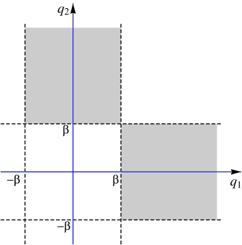
Figure 1: Regions of variations of the parameters $q_{1}$ and $q_{2}$ (see Eq. (26)) corresponding to the conditions of positivity of the densities $\rho_{1}$ and $\rho_{2}$ defined by Eqs. (15).

Formal integration of the system (24) yields

$$\begin{split}&\int_{q_{10}}^{q}\frac{dq}{\sqrt{\mathcal{R}(q)}}+\int_{q_{20}}^{q_{2}}\frac{dq}{\sqrt{\mathcal{R}(q)}}=0,\\ &\int_{q_{10}}^{q}\frac{qdq}{\sqrt{\mathcal{R}(q)}}+\int_{q_{20}}^{q_{2}}\frac{qdq}{\sqrt{\mathcal{R}(q)}}=\pm 2{\xi},\end{split}$$ (27)

where $q_{10}$ and $q_{20}$ are integration constants equal to the values of $q_{1}$ and $q_{2}$ at $\xi=0$, respectively. Every solution of the system (24) is parameterized by five zeroes $\nu_{i}$, $i=1,\ldots,5$, of the polynomial

$$\mathcal{R}(q)=\prod_{i=1}^{5}(q-\nu_{i})$$ (28)

and, depending on their values, we obtain different classes of solutions. Since the solution is symmetric with respect to transposition of $q_{1}$ and $q_{2}$, for definiteness we assume that they change in the intervals (the zeroes $\nu_{i}$ are numerated in the order of their values)

$$\nu_{1}\leq q_{1}\leq\nu_{2}\quad\text{and}\quad\nu_{3}\leq q_{2}\leq\nu_{4}$$ (29)

where the polynomial $\mathcal{R}(q)$ is positive.

III.1 Limit $\beta\to 0$

If $\beta\equiv\beta_{1}-\beta_{2}\to 0$, then we must have $\nu_{1}\to 0$ and $\nu_{2}\to 0$ to satisfy the conditions (26). At the same time, to get in this singular limit from Eqs. (15) finite values of $\rho_{1}$ and $\rho_{2}$, we have to define new variables and parameters as

$$q_{1}=\beta\widetilde{q}_{1},\quad\nu_{1}=\beta\widetilde{\nu}_{1},\quad\nu_{2}=\beta\widetilde{\nu}_{2}$$ (30)

so that Eqs. (15) reduce to

$$\rho_{1}=\frac{1}{2}q_{2}(1+\widetilde{q}_{1}),\quad\rho_{2}=\frac{1}{2}q_{2}(1-\widetilde{q}_{1}).$$ (31)

The Kowalevski equations (25) are then transformed to

$$\begin{split}\frac{d\widetilde{q}_{1}}{d\xi}&=\frac{2\sqrt{\nu_{3}\nu_{4}\nu_{5}}}{q_{2}}\sqrt{(\widetilde{q}_{1}-\widetilde{\nu}_{1})(\widetilde{\nu}_{2}-\widetilde{q}_{2})},\\ \frac{dq_{2}}{d\xi}&=-2\sqrt{(q_{2}-\nu_{3})(\nu_{4}-q_{2})(\nu_{5}-q_{2})}.\end{split}$$ (32)

We notice that the expression $\rho\equiv\rho_{1}+\rho_{2}=q_{1}+q_{2}$ reduces to $\rho=q_{2}$ in this limit. Introducing also $\widetilde{q}_{1}=\cos\theta$, $\widetilde{\nu}_{1}=\cos\theta_{1}$, $\widetilde{\nu}_{2}=\cos\theta_{2}$, $\nu_{3}=\rho_{1}$, $\nu_{4}=\rho_{2}$, $\nu_{5}=\rho_{3}$, we arrive at the equations

$$\begin{split}\frac{d\cos\theta}{d\xi}&=-\frac{2\sqrt{\rho_{1}\rho_{2}\rho_{2}}}{\rho}\sqrt{(\cos\theta-\cos\theta_{1})(\cos\theta_{2}-\cos\theta)},\\ \frac{d\rho}{d\xi}&=-2\sqrt{(\rho-\rho_{1})(\rho_{2}-\rho)(\rho_{3}-\rho)}\end{split}$$ (33)

identical to the equation obtained for this special case in Refs. wright-13 ; kamch-13 ; kamch-14 ; kamch-14b .

It is worth noticing that the integrals of motion (13) and (14) can be cast after introduction of these new variables $\rho$ and $\theta$ to the form

$$\begin{split}&H=\frac{\rho_{\xi}^{2}}{8\rho}-\frac{\rho^{2}}{2}+\tilde{\beta}\rho\\ &+\frac{\rho^{2}\sin^{2}\theta\cdot\theta_{\xi}^{2}+8[\alpha_{1}^{2}+\alpha_{2}^{2}-(\alpha_{1}^{2}-\alpha_{2}^{2})\cos\theta]}{8\rho\sin^{2}\theta}=h,\end{split}$$ (34)

$$\begin{split}K=&\frac{\rho^{2}\sin^{2}\theta\cdot\theta_{\xi}^{2}+8[\alpha_{1}^{2}+\alpha_{2}^{2}-(\alpha_{1}^{2}-\alpha_{2}^{2})\cos\theta]}{4\sin^{2}\theta}\\ &-(\alpha_{1}+\alpha_{2})^{2}=k.\end{split}$$ (35)

The angle $\theta$ can be excluded from Eq. (34) with the use of Eq. (35) what gives the equation for a single variable $\rho$,

$$\rho_{\xi}^{2}=4\rho^{3}-8\tilde{\beta}\rho^{2}+8h\rho-4[k+(\alpha_{1}+\alpha_{2})^{2}]$$ (36)

which is another form of the second equation (33). Its solution can be expressed in terms of elliptic functions. When $\rho$ is known, then $\theta=\theta(\xi)$ can be obtained by integration of the equation (35) or

$$\theta_{\xi}^{2}=\frac{8}{\rho^{2}}\left[\frac{k+(\alpha_{1}+\alpha_{2})^{2}}{2}-\frac{\alpha_{1}^{2}+\alpha_{2}^{2}-(\alpha_{1}^{2}-\alpha_{2}^{2})\cos\theta}{\sin^{2}\theta}\right],$$ (37)

which also coincides up to the notation with the first equation (33). When their solutions are found then the components densities are given by (31) transformed to

$$\rho_{1}(\xi)=\rho(\xi)\cos^{2}\frac{\theta(\xi)}{2},\quad\rho_{2}(\xi)=\rho(\xi)\sin^{2}\frac{\theta(\xi)}{2}$$ (38)

More details about these solutions can be found in Refs. wright-13 ; kamch-13 ; kamch-14 ; kamch-14b . In particular, they include also the well-known Manakov dark-dark soliton solution.

III.2 Appelrot-Delone class of solutions

The systems (24) and (25) were applied for the first time to a real mechanical problem by Sophie Kowalevski in her theory of rotation of the so-called Kowalevski top kow-1889 . After that some particular especially remarkable motions of this top were discussed by other authors, in particular, by G. G. Appelrot and N. B. Delone (see, e.g., golubev ). Here we shall apply their method to the special case of nonlinear motion of a two-component BEC which we shall also call the Appelrot-Delone case.

Let us suppose that the polynomial $\mathcal{R}(q)$ has a double root $q=\bar{\nu}$, the other roots we denote $\nu_{1}\leq\nu_{2}\leq\nu_{3}$, that is we have

$$\mathcal{R}(q)=(q-\bar{\nu})^{2}(q-\nu_{1})(q-\nu_{2})(q-\nu_{3})\equiv(q-\bar{\nu})^{2}\mathcal{R}_{1}(q),$$ (39)

where $\mathcal{R}_{1}(q)$ is the 3rd degree polynomial with the roots $\nu_{1},\,\nu_{2},\,\nu_{3}$. In this case it is convenient to use the system (25) written now in the form

$$\begin{split}2(q_{1}-\bar{\nu})\sqrt{\mathcal{R}_{1}(q_{1})}&=(q_{1}-q_{2})\frac{dq_{1}}{d\xi},\\ 2(q_{2}-\bar{\nu})\sqrt{\mathcal{R}_{1}(q_{2})}&=-(q_{1}-q_{2})\frac{dq_{2}}{d\xi}.\end{split}$$ (40)

It is easy to see that this system is satisfied if

$$\begin{split}&q_{1}=\bar{\nu},\quad\frac{dq_{2}}{d\xi}=2\sqrt{\mathcal{R}_{1}(q_{2})}\\ \text{or}\quad&q_{2}=\bar{\nu},\quad\frac{dq_{1}}{d\xi}=2\sqrt{\mathcal{R}_{1}(q_{1})}.\end{split}$$ (41)

Both solutions lead to the same physical solution due to symmetry of Eqs. (15) with respect to transposition of $q_{1}$ and $q_{2}$. For definiteness we shall take the second solution in (41). Then the variable $q_{1}$ oscillates in the interval $\nu_{1}\leq q_{1}\leq\nu_{2}$, where $\mathcal{R}_{1}(q_{1})\geq 0$ and, hence, for $\beta>0$, we have according to (26) two choices for the parameters $\bar{\nu},\,\nu_{1},\,\nu_{2}$,

$$\begin{split}&\beta\leq\nu_{1}<\nu_{2},\quad-\beta\leq\bar{\nu}\leq\beta\\ -&\beta\leq\nu_{1}<\nu_{2}\leq\beta,\quad\bar{\nu}\geq\beta.\end{split}$$ (42)

As we shall see, the second choice cannot give the soliton solution, so we shall consider the first one.

In standard way we obtain

$$q_{1}(\xi)=\nu_{1}+(\nu_{2}-\nu_{1})\mathrm{sn}^{2}(\sqrt{\nu_{3}-\nu_{1}}\,(\xi-\xi_{0}),m),$$ (43)

where

$$m=\frac{\nu_{2}-\nu_{1}}{\nu_{3}-\nu_{1}},$$ (44)

and, to simplify the notation, from now on we shall put the integration constant $\xi_{0}=0$. Then the components densities are given by

$$\begin{split}&\rho_{1}=\frac{\bar{\nu}+\beta}{2\beta}[\beta+\nu_{1}+(\nu_{2}-\nu_{1})\mathrm{sn}^{2}(\sqrt{\nu_{3}-\nu_{1}}\,\xi,m)],\\ &\rho_{2}=\frac{\bar{\nu}-\beta}{2\beta}[\beta-\nu_{1}-(\nu_{2}-\nu_{1})\mathrm{sn}^{2}(\sqrt{\nu_{3}-\nu_{1}}\,\xi,m)],\end{split}$$ (45)

and their substitution into (7) yields the flow velocities. These formulae represent the periodic nonlinear wave which can be called the density wave, since the densities oscillate in phase and in the small amplitude limit this wave reduces to the sound wave, which describes oscillations of the total density $\rho=\rho_{1}+\rho_{2}$.

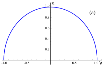
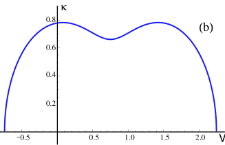
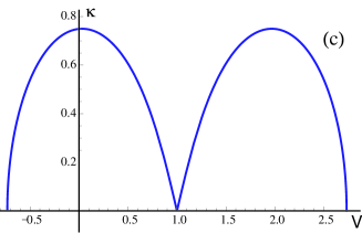
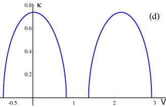
Figure 2: Dependence of the inverse width $\kappa$ of a dark-dark soliton on its velocity $V$ for different values of the relative velocity between condensates. In all plots $\rho_{10}=\rho_{20}=0.5$, $u_{10}=0$ and $V$ is measured with respect to quiescent condensate: (a) $u_{20}=0$, this is the case of well-known dark-dark solitons propagating through two still condensates; (b) plot corresponding to $u_{20}=1.5$ illustrates a non-monotonic dependence; (c) at $u_{20}=2.0$ the region of possible velocities splits with formation of two disconnected regions; (d) plot for $u_{20}=2.2$ illustrates appearance of two disconnected regions of possible soliton velocities $V$.

Let us consider the soliton limit when $\nu_{3}\to\nu_{2}$ ($m\to 1$):

$$\begin{split}&\rho_{1}=\frac{\bar{\nu}+\beta}{2\beta}\left(\beta+\nu_{2}-\frac{\nu_{2}-\nu_{1}}{\cosh^{2}(\sqrt{\nu_{2}-\nu_{1}}\xi)}\right),\\ &\rho_{2}=\frac{\bar{\nu}-\beta}{2\beta}\left(\beta-\nu_{2}+\frac{\nu_{2}-\nu_{1}}{\cosh^{2}(\sqrt{\nu_{2}-\nu_{1}}\xi)}\right),\end{split}$$ (46)

where $\beta<\nu_{1}<\nu_{2}$ and $-\beta<\bar{\nu}<\beta$. These parameters can be expressed in terms of the constant densities at $|\xi|\to\infty$,

$$\rho_{10}=\frac{1}{2\beta}(\bar{\nu}+\beta)(\beta+\nu_{2}),\quad\rho_{20}=\frac{1}{2\beta}(\bar{\nu}-\beta)(\beta-\nu_{2}).$$ (47)

Solving this system with respect to $\nu_{2}$ and $\bar{\nu}$ gives

$$\begin{split}\nu_{2}&=\frac{1}{2}\left(\rho_{10}+\rho_{20}-\sqrt{(\rho_{10}-\rho_{20}-2\beta)^{2}+4\rho_{10}\rho_{20}}\right),\\ \bar{\nu}&=\frac{1}{2}\left(\rho_{10}+\rho_{20}+\sqrt{(\rho_{10}-\rho_{20}-2\beta)^{2}+4\rho_{10}\rho_{20}}\right).\end{split}$$ (48)

The parameter $\beta$ can be also expressed in terms of $\rho_{10},\,\rho_{20}$ and constant flow velocities $u_{10},\,u_{20}$ at $|\xi|\to\infty$. From (7) and (8) we get

$$\alpha_{1}=\rho_{10}(u_{10}-V),\quad\alpha_{2}=\rho_{20}(u_{20}-V)$$ (49)

and

$$\begin{split}\beta_{1}&=\frac{1}{2}(u_{10}-V)^{2}+\rho_{10}+\rho_{20},\\ \beta_{2}&=\frac{1}{2}(u_{20}-V)^{2}+\rho_{10}+\rho_{20},\end{split}$$ (50)

hence

$$\beta=\frac{1}{2}\left[(u_{10}-V)^{2}-(u_{20}-V)^{2}\right].$$ (51)

To determine the last unknown parameter $\nu_{1}$, we remark that Viète formula for the polynomial (23) in our case gives $\beta_{1}+\beta_{2}=\nu_{1}+2(\nu_{2}+\bar{\nu})$ and, consequently,

$$\nu_{1}=\frac{1}{2}\left[(u_{10}-V)^{2}+(u_{20}-V)^{2}\right].$$ (52)

The solution (46) exists if $\nu_{2}>\nu_{1}$ and this condition gives restrictions for the soliton velocity,

$$\frac{\rho_{10}}{(V-u_{10})^{2}}+\frac{\rho_{20}}{(V-u_{20})^{2}}>1.$$ (53)

Note that for the second choice in (42) the condition $\nu_{2}>\nu_{1}$ cannot be fulfilled. In the limiting case of one-component quiescent condensate ($\rho_{20}=0,\,u_{10}=0$) the condition (53) reduces to the well-known fact that the soliton velocity is smaller than the sound velocity, $V<c_{s}=\sqrt{\rho_{10}}$.

Dependence of the inverse width $\kappa=\sqrt{\nu_{2}-\nu_{1}}$ of soliton on its velocity $V$ is given by

$$\begin{split}&\kappa=\frac{1}{\sqrt{2}}\Big{\{}\rho_{10}+\rho_{20}-(u_{10}-V)^{2}-(u_{20}-V)^{2}\\ &+\sqrt{[\rho_{10}-\rho_{20}-(u_{10}-V)^{2}+(u_{20}-V)^{2}]^{2}+4\rho_{10}\rho_{20}}\Big{\}}^{1/2}.\end{split}$$ (54)

This expression can be also obtained by linearization of equations (8) with respect to small deviations $\rho_{k}^{\prime}$ around asymptotic densities ($\rho_{k}=\rho_{k0}+\rho_{k}^{\prime}$) and seeking the solution of the linearized equations in the form $\rho_{k}^{\prime}\propto\exp(-\kappa|\xi|)$. This calculation shows that the Appelrot-Delone class of solutions yields in the corresponding limit all soliton solutions with exponentially decaying tails around non-zero background densities $\rho_{k0}\neq 0$.

Dependence (54) is illustrated in Fig. 2 for different values of the relative velocity of the BEC components. The remarkable new feature is that this dependence can be non-monotonic and for large enough values of the relative velocity the region of possible values of the velocity $V$ splits into two separated regions in sharp contrast with the one-component situation. The appearance of two regions of velocity can be illustrated graphically in the following way. We introduce for convenience the variables $X=V-u_{10}$, $Y=V-u_{20}$; then the boundary of the region (53) is given by the equation

$$X^{2}Y^{2}-\rho_{10}Y^{2}-\rho_{20}X^{2}=0.$$ (55)

Its plot is shown in Fig. 3 by a solid line and the admissible values of $V$ are located inside this line (that is in the area including the origin of the coordinate system). If we fix the value of the relative velocity $U_{0}=u_{20}-u_{10}\equiv X-Y$, then the possible values of $V$ correspond to points of the straight line located between its intersections with the curve (55). Consequently, the splitting of the region of possible values of $V$ correspond to such $U_{0}$ that the straight line $X-Y=U_{0}$ touches the curve (55) at the point where $dY/dX=1$ or

$$XY^{2}+X^{2}Y-\rho_{10}Y-\rho_{20}X=0$$ (56)

(see Fig. 3). The system (55) and (56) can be easily solved to give

$$\begin{split}&X=V-u_{10}=\pm\rho_{10}^{1/3}\sqrt{\rho_{10}^{1/3}+\rho_{20}^{1/3}},\\ &Y=V-u_{20}=\mp\rho_{20}^{1/3}\sqrt{\rho_{10}^{1/3}+\rho_{20}^{1/3}},\end{split}$$ (57)

and hence the critical value of the relative velocity is given by

$$U_{0}=(\rho_{10}^{1/3}+\rho_{20}^{1/3})^{3/2}.$$ (58)

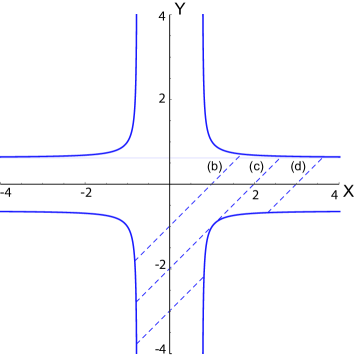
Figure 3: Plot of the curve (64) (solid line) and of the straight lines $X-Y=U_{0}$ (dashed lines): (b) corresponds to a single region of possible values of $V$ (see Fig. 2b); (c) correspond to the relative velocity at which the region splits into two regions (see Fig. 2c); (d) corresponds to two separated regions (see Fig. 2d).

III.3 Dark-bright soliton solution

If one of the background densities vanishes (say, $\rho_{20}=0$), then the so-called dark-bright soliton solutions of the Manakov system are obtained (see, e.g., sk-1997 ; smkj-10 ). Here we show that this type of solutions is a specialization of general solutions of the Kowalevski equations when the polynomial $\mathcal{R}(q)$ has two double zeroes. In this case the condition (29) is fulfilled if one of the double zeroes coincides with $\beta$. Thus, we assume that

$$-\beta\leq\nu_{1}\leq q_{1}\leq\beta\quad\text{and}\quad\beta\leq q_{2}\leq\bar{\nu}=\nu_{4}=\nu_{5}.$$ (59)

Then the system (25) reduces to

$$\begin{split}2(\beta-q_{1})(\bar{\nu}-q_{1})\sqrt{q_{1}-\nu_{1}}&=(q_{1}-q_{2})\frac{dq_{1}}{d\xi},\\ 2(q_{2}-\beta)(\bar{\nu}-q_{2})\sqrt{q_{2}-\nu_{1}}&=-(q_{1}-q_{2})\frac{dq_{2}}{d\xi}.\end{split}$$ (60)

As in the preceding subsection, we see that the second equation is satisfied identically by $q_{2}=\bar{\nu}$ and the first equation $dq_{1}/d\xi=-2(\beta-q_{1})\sqrt{q_{1}-\nu_{1}}$ can be easily integrated to give $q_{1}=\beta-(\beta-\nu_{1})\cosh^{-2}(\sqrt{\beta-\nu_{1}}\,\xi).$ As a result we obtain the densities

$$\begin{split}\rho_{1}&=(\bar{\nu}+\beta)\left(1-\frac{(\beta-\nu_{1})/(2\beta)}{\cosh^{2}(\sqrt{\beta-\nu_{1}}\,\xi)}\right),\\ \rho_{2}&=(\bar{\nu}-\beta)\cdot\frac{(\beta-\nu_{1})/(2\beta)}{\cosh^{2}(\sqrt{\beta-\nu_{1}}\,\xi)}\end{split}$$ (61)

which obviously correspond to the dark-bright soliton: the density $\rho_{1}$ has a dip at $\xi=0$ and approaches to the background density $\rho_{0}=\bar{\nu}+\beta$ as $|\xi|\to\infty$ whereas $\rho_{2}$ has a hump at $\xi=0$ and vanishes as $|\xi|\to\infty$. Let us relate the parameters of formulae (61) with standard physical parameters for the soliton solution. To this end we define the inverse half-width $\kappa$ of the soliton by the equation $\kappa=\sqrt{\beta-\nu_{1}}$ and introduce the ratio of the components densities at the center of the soliton $\gamma=(\rho_{0}-\rho_{1}(0))/\rho_{2}(0)=(\bar{\nu}+\beta)/(\bar{\nu}-\beta)$. Besides that we assume that there is no flow of the first component at infinity: $u_{10}=0$. Then from Eqs. (7) and (8) we find $\alpha_{1}=-V\rho_{0}$, $\alpha_{2}=0$, $\beta_{1}=\rho_{0}+V^{2}/4$, $\beta_{2}=\rho_{0}-\kappa^{2}/2$ and hence

$$\beta=\frac{V^{2}}{4}+\frac{\kappa^{2}}{2}=\rho_{0}\frac{\gamma-1}{2\gamma},\quad\nu_{1}=\beta-\kappa^{2},\quad\bar{\nu}=\rho_{0}\frac{\gamma+1}{2\gamma}.$$ (62)

The dependence of the soliton’s inverse width on its velocity is given by the formula

$$\kappa(V)=\sqrt{\frac{\gamma-1}{\gamma}\rho_{0}-\frac{V^{2}}{2}}.$$ (63)

These formulae are equivalent to those found in Ref. sk-1997 .

III.4 Legendre-Jacobi class of solutions

The general one-phase traveling waves described by the Manakov system can be illustrated by an easy numerical solutions of the Kowalevski equations (25). On the other hand, the analytical solution (27) can be expressed in terms of Riemann $\theta$-functions by the methods used already by S. Kowalevski (see kow-1889 ; golubev ) and developed further in the algebraic-geometric approach to integrable equations (see, e.g., bbeim ). This method was applied to the one-phase solutions of the focusing Manakov system in Refs. cezk-2000 ; eek-2000 . However, the resulting expressions are quite inconvenient for practical use. Therefore we shall confine ourselves here to a particular case, when the solution can be reduced to the much better known special functions (elliptic integrals) which permit one to understand the characteristic features of the solution in a much simpler way. Here we shall consider such a situation first noticed by Legendre legendre and generalized by Jacobi jacobi-1832 .

Let the zeroes of the polynomial $\mathcal{R}(q)$ be given by

$$\begin{split}&\nu_{1}=c-1/b,\quad\nu_{2}=c-1/a,\quad\nu_{3}=c,\\ &\nu_{4}=c+1,\quad\nu_{5}=c+1/ab,\end{split}$$ (64)

where $0<b\leq a\leq 1$ and the parameter $c$ satisfies the conditions

$$\mathrm{max}\{\beta,\,1/b-\beta\}<c<\beta+1/a.$$ (65)

so that $q_{1}$ and $q_{2}$ oscillate within the intervals

$$-\beta<\nu_{1}\leq q_{1}\leq\nu_{2}<\beta,\quad\beta<\nu_{3}\leq q_{2}\leq\nu_{4}.$$ (66)

Let us assume for definiteness that at $\xi=0$ we have $q_{1}(0)=c-1/a$ and $q_{2}=c$ (other choices of the initial conditions can be considered in a similar way). Then, introducing the variables

$$z_{1,2}=q_{1,2}-c,$$ (67)

we represent the solution (27) in the form

$$\begin{split}&\int_{-1/a}^{z_{1}}\frac{dz}{\sqrt{\widetilde{\mathcal{R}}(z)}}+\int_{0}^{z_{2}}\frac{dz}{\sqrt{\widetilde{\mathcal{R}}(z)}}=0,\\ &\int_{-1/a}^{z_{1}}\frac{zdz}{\sqrt{\widetilde{\mathcal{R}}(z)}}+\int_{0}^{z_{2}}\frac{zdz}{\sqrt{\widetilde{\mathcal{R}}(z)}}=\pm 2{\xi},\end{split}$$ (68)

where

$$\widetilde{\mathcal{R}}(z)=z(1-z)(1-abz)((1+az)(1+bz)/(ab)^{2}.$$ (69)

As Jacobi showed jacobi-1832 , the integrals here can be calculated in terms of incomplete elliptic integrals of the first kind. Since Jacobi did not provide the details of his method, this calculation is discussed briefly in Appendix. As a result, we obtain a particular solution of Eqs. (24) in the form

$$\begin{split}&F(\varphi_{1a},k_{1})+F(\varphi_{1b},k_{2})-F(\varphi_{2},k_{1})-F(\varphi_{2},k_{2})=0,\\ &F(\varphi_{1a},k_{1})-F(\varphi_{1b},k_{2})-F(\varphi_{2},k_{1})+F(\varphi_{2},k_{2})\\ &=\pm 2\sqrt{\frac{(1+a)(1+b)}{ab}}\,\xi,\end{split}$$ (70)

where

$$\varphi_{1a}=\left\{\begin{array}[]{l}\pi-\arcsin\sqrt{\frac{(1+az_{1})(1+bz_{1})}{z_{1}(\sqrt{a}-\sqrt{b})^{2}}},\quad-\frac{1}{b}\leq z_{1}\leq-\frac{1}{\sqrt{ab}},\\ \arcsin\sqrt{\frac{(1+az_{1})(1+bz_{1})}{z_{1}(\sqrt{a}-\sqrt{b})^{2}}},\quad-\frac{1}{\sqrt{ab}}\leq z_{1}\leq-\frac{1}{a};\end{array}\right.$$ (71)

$$\varphi_{1b}=\arcsin\sqrt{\frac{(1+az_{1})(1+bz_{1})}{z_{1}(\sqrt{a}+\sqrt{b})^{2}}},\quad-\frac{1}{b}\leq z_{1}\leq-\frac{1}{a};$$ (72)

$$\varphi_{2}=\arcsin\sqrt{\frac{(1+a)(1+b)z_{2}}{(1+az_{2})(1+bz_{2})}},\quad 0\leq z_{2}\leq 1.$$ (73)

These equations determine implicitly the dependence of $z_{1}$ and $z_{2}$, and, hence, of $q_{1}$ and $q_{2}$, on $\xi$ in the interval of $\xi$ until the first turning point is met ($z_{1}=-1/b$ or $z_{2}=1$). After that the sign before the corresponding square root in the Kowalevski equations (25) must be changed and the replacement in the solution (68)

$$\int_{-1/a}^{z_{1}}\frac{dz}{\sqrt{\widetilde{\mathcal{R}}(z)}}\to\int_{-1/a}^{-1/b}\frac{dz}{\sqrt{\widetilde{\mathcal{R}}(z)}}-\int_{-1/b}^{z_{1}}\frac{dz}{\sqrt{\widetilde{\mathcal{R}}(z)}}$$

or

$$\int_{0}^{z_{2}}\frac{dz}{\sqrt{\widetilde{\mathcal{R}}(z)}}\to\int_{0}^{1}\frac{dz}{\sqrt{\widetilde{\mathcal{R}}(z)}}-\int_{1}^{z_{2}}\frac{dz}{\sqrt{\widetilde{\mathcal{R}}(z)}}$$

must be done with similar changes in the expressions (70). Making such changes at every successive turning point, we find the solution in any necessary interval of $\xi$. Substitution of resulting $q_{1}=z_{1}+c$ and $q_{2}=z_{2}+c$ into Eqs. (15) yields the dependence of densities $\rho_{1}$ and $\rho_{2}$ on $\xi$. Typical resulting plots are shown in Fig. 4.

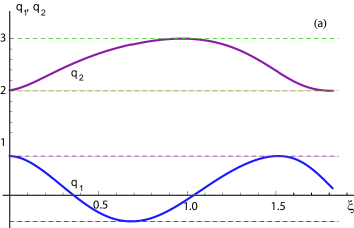
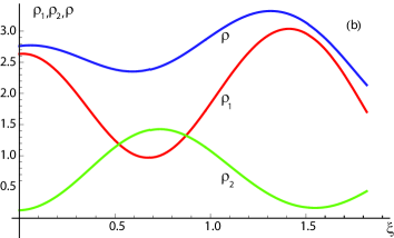
Figure 4: (Color online) Plots for the solution (70) of the Kowalevski equations for the values of the parameters $a=0.8$, $b=0.4$, $c=2$ which correspond to $\nu_{1}=-0.5$, $\nu_{2}=0.75$, $\nu_{3}=2.0$, $\nu_{3}=3.0$, $\nu_{5}=5.125$. The initial conditions are given by $q_{1}(0)=\lambda_{2}$, $q_{2}(0)=\lambda_{3}$. (a) Plots of $q_{1}$ and $q_{2}$ for the interval of $\xi$ corresponding to full cycle of $q_{2}$-variable; dashed lines indicate the values of $\nu_{i}$, $i=1,2,3,4$; (b) plots of the components densities $\rho_{1}$ and $\rho_{2}$ and of the total density $\rho=\rho_{1}+\rho_{2}$.

As one can see in Fig. 4, in the general solution the periodicity of the wave in space and time is lost and the wave pattern demonstrates quite complicated behavior as a function of $\xi$.

IV Conclusion

In this paper we have found the one-phase traveling wave solution of the Manakov system which describes evolution of two-component BEC. It is shown that in this case the Manakov system reduces to the equations which S. Kowalevski derived in her study of rotation of a heavy top in the discovered by her completely integrable case. We show that the previously found solutions of the Manakov system appear in this scheme as particular cases. Besides that, new solutions are found which were either missed in previous analysis or cannot be obtained by more elementary methods when parameters of the solutions are chosen in such a way that the evolution equations are greatly simplified. In particular, we have found a new dark-dark soliton solution for a two-component BEC with the non-zero relative motion of the components. This solution has very unusual dependence of the inverse width on the soliton’s velocity. In principle, this can lead to new forms of dispersive shock waves evolved from initial step-like distributions of the components densities or velocities.

For applications of the developed theory to the description of the polarization wave patterns observed in the experiments hamner-11 ; hoefer-11 ; hamner-13 , the Whitham modulation theory whitham ; kamch-2000 for these waves has to be developed. Some particular situations have already been studied in Refs. wright-95 (genus-zero case) and kamch-14b (genus-one case for the limit $\beta=0$). The results of the present paper demonstrate that the general one-phase solution is described by the fifth-degree polynomial $\mathcal{R}(q)$ whose zeroes as well as the wave velocity must be related in framework of the finite-gap integration method with the modulation parameters appearing in the Whitham theory of modulations of nonlinear waves. Thus, the results obtained here provide the necessary step to development of the modulation theory which can be applied to description of dispersive polarization shock waves observed experimentally. Derivation of the Whitham equations is a difficult problem far beyond the scope of this paper and we hope to consider it elsewhere.

Appendix

We have to calculate the integrals

$$\begin{split}&I_{1}=\int_{0}^{z}\frac{dz}{\sqrt{\widetilde{\mathcal{R}}(z)}},\quad I_{1}^{\prime}=\int_{0}^{z}\frac{zdz}{\sqrt{\widetilde{\mathcal{R}}(z)}},\\ &I_{2}=\int_{-1/a}^{z}\frac{dz}{\sqrt{\widetilde{\mathcal{R}}(z)}},\quad I_{2}^{\prime}=\int_{-1/a}^{z}\frac{zdz}{\sqrt{\widetilde{\mathcal{R}}(z)}}.\end{split}$$ (A.1)

The integrals $I_{1}$ and $I_{1}^{\prime}$ are calculated with the use of the substitution

$$1+abz^{2}=uz$$ (A.2)

or

$$\sqrt{z}=\left(\sqrt{u+2\sqrt{ab}}\pm\sqrt{u-2\sqrt{ab}}\right)/(2\sqrt{ab}),$$ (A.3)

where $u$ is a new integration variable. It is easy to see that the function (A.3) with the lower sign maps the interval $1+ab\leq u<\infty$ on $0\leq z\leq 1$ and with the upper sign maps the same interval on $1/(ab)\leq z<\infty$. Then substitution (A.3) with the lower sign into $I_{1}$ gives after simple manipulations

$$\begin{split}I_{1}&=\frac{ab}{2}\int_{u(z)}^{\infty}\frac{du}{\sqrt{(u+a+b)(u+2\sqrt{ab})(u-1-ab)}}\\ &+\frac{ab}{2}\int_{u(z)}^{\infty}\frac{du}{\sqrt{(u+a+b)(u-2\sqrt{ab})(u-1-ab)}},\end{split}$$ (A.4)

where

$$u(z)=(1+abz^{2})/z.$$ (A.5)

Elliptic integrals in (A.4) are transformed to the standard form by the substitution

$$u=\frac{(1+a)(1+b)}{\sin^{2}\varphi}-a-b.$$ (A.6)

As a result we obtain

$$I_{1}=\frac{ab}{\sqrt{(1+a)(1+b)}}\left\{F(\varphi,k_{1})+F(\varphi,k_{2})\right\},$$ (A.7)

where $F(\varphi,k)$ denotes the elliptic integral of the first kind,

$$k_{1}=\frac{\sqrt{a}-\sqrt{b}}{\sqrt{(1+a)(1+b)}},\quad k_{2}=\frac{\sqrt{a}+\sqrt{b}}{\sqrt{(1+a)(1+b)}},$$ (A.8)

and $\varphi$ is related with the upper limit of integration $z$ by the formula

$$\sin^{2}\varphi=\frac{(1+a)(1+b)z}{(1+az)(1+bz)}.$$ (A.9)

The integral $I_{1}^{\prime}$ is calculated by the same method and the result reads

$$I_{1}^{\prime}=\sqrt{\frac{ab}{(1+a)(1+b)}}\left\{-F(\varphi,k_{1})+F(\varphi,k_{2})\right\}.$$ (A.10)

The integrals $I_{2}$ and $I_{2}^{\prime}$ in (A.1) can be calculated with the use of the substitution

$$u(z)=-(1+abz^{2})/z$$ (A.11)

or

$$\sqrt{-z}=\left(\sqrt{u+2\sqrt{ab}}\pm\sqrt{u-2\sqrt{ab}}\right)/(2\sqrt{ab}),$$ (A.12)

which map the interval $2\sqrt{ab}\leq u\leq a+b$ on the intervals $-1/b\leq z\leq-1/\sqrt{ab}$ and $-1/\sqrt{ab}\leq z\leq-1/a$, correspondingly for upper and lower signs. This transforms $I_{2}$ to

$$\begin{split}I_{2}&=\frac{ab}{2}\int_{a+b}^{u(z)}\frac{du}{\sqrt{(u-a-b)(u+2\sqrt{ab})(u+1+ab)}}\\ &+\frac{ab}{2}\int_{a+b}^{u(z)}\frac{du}{\sqrt{(u-a-b)(u-2\sqrt{ab})(u+1+ab)}}.\end{split}$$ (A.13)

These integrals are reduced to standard form of elliptic integrals by substitutions

$$u=a+b-(a+b\pm 2\sqrt{ab})\sin^{2}\varphi.$$ (A.14)

As a result we obtain

$$I_{2}=-\frac{ab}{\sqrt{(1+a)(1+b)}}\left\{F(\varphi_{a},k_{1})+F(\varphi_{b},k_{2})\right\},$$ (A.15)

where

$$\varphi_{a}=\left\{\begin{array}[]{l}\pi-\arcsin\sqrt{\frac{(1+az)(1+bz)}{z(\sqrt{a}-\sqrt{b})^{2}}},\quad-\frac{1}{b}\leq z\leq-\frac{1}{\sqrt{ab}},\\ \arcsin\sqrt{\frac{(1+az)(1+bz)}{z(\sqrt{a}-\sqrt{b})^{2}}},\quad-\frac{1}{\sqrt{ab}}\leq z\leq-\frac{1}{a};\end{array}\right.$$ (A.16)

and

$$\varphi_{b}=\arcsin\sqrt{\frac{(1+az)(1+bz)}{z(\sqrt{a}+\sqrt{b})^{2}}},\quad-\frac{1}{b}\leq z\leq-\frac{1}{a}.$$ (A.17)

Similar calculation yields

$$I_{2}^{\prime}=\sqrt{\frac{ab}{(1+a)(1+b)}}\left\{F(\varphi_{a},k_{1})-F(\varphi_{b},k_{2})\right\}.$$ (A.18)

References

- (1) M. Abad, A. Recati, Eur. Phys. J. D 67, 148 (2013).
- (2) Yu. G. Gladush, A. K. Kamchatnov, Z. Shi, P. G. Kevrekidis, D. J. Frantzeskakis, B. A. Malomed, Phys. Rev. A 79, 033623 (2009).
- (3) A. M. Kamchatnov, Y. V. Kartashov, Phys. Rev. Lett. 111, 140402 (2013).
- (4) C. Hamner, J. J. Chang, P. Engels, M. A. Hoefer, Phys. Rev. Lett. 106, 065302 (2011).
- (5) M. A. Hoefer, J. J. Chang, C. Hamner, P. Engels, Phys. Rev. A 84, 041605(R) (2011).
- (6) C. Hamner, Y. Zhang, J. J. Chang, C. Zhang, P. Engels, Phys. Rev. Lett. 111, 264101 (2013).
- (7) S. V. Manakov, Zh. Eksp. Teor. Fiz., 65, 505 (1973) [Sov. Phys. JETP 38, 248 (1974)].
- (8) A. L. Berkhoer and V. E. Zakharov, Zh. Eksp. Teor. Fiz., 58, 903 (1970) [Sov. Phys. JETP 31, 486 (1970)].
- (9) Yu. S. Kivshar and G. P. Agrawal, Optical Solitons: From Fibers to Photonic Crystals, (Academic, San Diego, 2003).
- (10) A. P. Sheppard and Y. S. Kivshar, Phys. Rev. E 55, 4773 (1997).
- (11) J. Smyrnakis, M. Magiropoulos, G. M. Kavoulakis, and A. D. Jackson, Phys. Rev. A 81, 063601 (2010).
- (12) O. C. Wright, Physica D 264, 1 (2013).
- (13) A. M. Kamchatnov, Europhys. Lett. 103, 60003 (2013).
- (14) A. M. Kamchatnov, Zh. Eksp. Teor. Fiz. 145, 719 (2014); [JETP, 118, 630 (2014)].
- (15) A. M. Kamchatnov, J. Phys. A: Math. Theor. 47, 145203 (2014).
- (16) S. Kowalevski, Acta Mathematica, 12, 177 (1889).
- (17) V. V. Golubev, Lectures on integration of the equations of motion of a rigid bode about a fixed point, (GITTL, Moscow, 1953) (in Russian) [English transl.: Israel Program Sci. Trans., Jerusalem, and Office of Tech. Services, U. S. Dept. Commerce, Washington, D.C., 1960].
- (18) C. Polymilis, K. Hizanidis, and D. J. Frantzeskakis, Phys. Rev. E 58, 1112 (1998).
- (19) P. L. Christiansen, J. C. Eilbeck, V. Z. Enolskii, and N. A. Kostov, Proc. roy. Soc. Lond. A 456, 2263 (2000).
- (20) J. C. Eilbeck, V. Z. Enolskii, and N. A. Kostov, J. Math. Phys., 41, 8236 (2000).
- (21) V. I. Arnold, Mathematical Methods of Classical Mechanics, (Springer, Berlin, 1989).
- (22) E. D. Belokolos, A. I. Bobenko, V. Z. Enol’skii, A. R. Its, V. B. Matveev, Algebro-Geometric Approach to Nonlinear Integrable Equations, (Springer, Berlin, 1994).
- (23) A. M. Legendre, Traité des Fonctions Elliptiques et des Integrales Eulériennes, t. 3, (Huzard-Courcier, Paris, 1828).
- (24) C. G. J. Jacobi, J. reine ang. Mat., 8, 413 (1832); Gesammelte Werke, Bd. 1, S. 373, (Chelsea, New York, 1969).
- (25) G. B. Whitham, Linear and Nonlinear Waves, (Wiley, New York, 1974).
- (26) A. M. Kamchatnov, Nonlinear Periodic Waves and Their Modulations: An Introductory Course (World Scientific, Singapore, 2000).
- (27) O. C. Wright, Physica D, 82, 1 (1995).