MEPSA: a flexible peak search algorithm designed for uniformly spaced time series

Abstract

We present a novel algorithm aimed at identifying peaks within a uniformly sampled time series affected by uncorrelated Gaussian noise. The algorithm, called “MEPSA” (multiple excess peak search algorithm), essentially scans the time series at different timescales by comparing a given peak candidate with a variable number of adjacent bins. While this has originally been conceived for the analysis of gamma–ray burst light (GRB) curves, its usage can be readily extended to other astrophysical transient phenomena, whose activity is recorded through different surveys. We tested and validated it through simulated featureless profiles as well as simulated GRB time profiles. We showcase the algorithm’s potential by comparing with the popular algorithm by Li and Fenimore, that is frequently adopted in the literature. Thanks to its high flexibility, the mask of excess patterns used by MEPSA can be tailored and optimised to the kind of data to be analysed without modifying the code. The C code is made publicly available.

1 Introduction

Transient phenomena are manifestation of various classes of astrophysical sources. Their study contributes to characterise the dynamics of such objects and gain clues on the physical processes responsible for their behaviour and evolution with time. In the current time domain era, most if not all transient sources are discovered and signal their transient character through the emission of one or multiple peaks in their flux time profile as a manifestation of enhanced activity. In high–energy astrophysics, for instance, this is the case for black–hole candidates in binary systems (e.g., Remillard and McClintock 2006), that of outbursting magnetars (e.g., Mereghetti 2008), or that of super fast X–ray transients (e.g., Sguera et al. 2005; Romano et al. 2014).

Moving to most energetic and disruptive events on stellar scales, gamma–ray bursts (GRBs) are no exception. Their gamma–ray time profiles, lasting from a fraction of a second all the way up to thousands seconds (Kouveliotou et al., 1993; Horváth et al., 2010; Levan et al., 2014), are characterised by a variable number of pulses with no firm evidence for periodicity. Such pulses often cluster within some emission episodes, separated by so–called quiescent times, during which the gamma–ray activity drops to the detector’s background level. The so–called GRB “prompt”, i.e. the gamma–ray emission itself, is still the least understood aspect of the GRB phenomenon: e.g., what is (or are) the gamma–ray emission mechanism(s), at what distance from the collapsing object, which kind of environment (see Kumar and Zhang 2014 for a recent review). One of the open issues concerns the stochastic (or deterministic?) process which rules the time profile and its complicated multi–pulse structure (Greco et al., 2011).

To tackle this, one must develop an effective technique to detect as many peaks as possible in the observed light curves to a reliable degree, properly accounting for the statistical uncertainties affecting the time series. Several authors in the GRB literature faced this problem building on different techniques: Li and Fenimore 1996 (hereafter, LF) set up a simple but effective algorithm based on the Poisson statistics affecting photon counting detectors. Other authors made extensive use of LF algorithm (Nakar and Piran, 2002; Drago and Pagliara, 2007; Bhat et al., 2012) to study the peak intensity as well as the distribution of waiting times, defined as the time intervals between adjacent pulses. In an alternative approach, Quilligan et al. (2002) set up a dedicated filter based on wavelets to suppress the statistical noise in GRB time profiles and study the basic statistical properties of pulses as a consequence. More recently, Charisi et al. (2014) studied the statistics of waiting times between emission episodes and precursor activity in GRBs observed by several past and present experiments by adapting an algorithm originally developed for gravitational data analysis. This is based on a combined time–frequency decomposition of the time series variance.

Motivated by the peak detection problem in GRB time series, in this paper we propose a new algorithm, called “multiple excess peak search algorithm” (hereafter, MEPSA), that is described in Sect. 2. As it will be shown in Sect. 3, compared with the previous LF algorithm and with a more conservative version of the same devised by us, MEPSA is characterised by a lower rate of false positive and a higher rate of true positive events, particularly for low signal–to–noise ratio (SNR) peaks. Moreover, thanks to its high flexibility, MEPSA can easily be adapted and tailored to different time series that are routinely obtained in many fields other than GRBs, without having to modify the code itself. A describes the output information provided by the code, which is made publicly available .

2 Algorithm’s description

MEPSA searches the input light curves for peaks by applying simultaneously a multi–pattern set of excesses, i.e. a set of $N=39$ patterns. The input time series must have uniform sampling and must be affected by statistical uncorrelated Gaussian noise. The series must be either background–subtracted, or removed of possible trends, so that changes in the expected value should only be due to signal and not to background. For each bin of the light curve, let $r_{i}$ the rates in the $i$-th bin. A given pattern $P_{k}$ ($k=1,\ldots,N$) consists of a fixed number of adjacent bins around the given $i$-th bin: around $i$ there are a given $n_{k,l}$ leftward bins (which temporally precede the $i$-th bin) and $n_{k,r}$ rightward bins (which temporally follow the $i$-th bin). The pattern assigns each of its bins, except for the $i$-th bin, a threshold $v_{k,j}$ ($j=1,\ldots,n_{k,l}+n_{k,r}$) in terms of number of $\sigma$’s (where $\sigma$ is the statistical noise corresponding to that bin). Pattern $P_{k}$ is then said to be fulfilled by bin $i$ when the following conditions are simultaneously fulfilled:

$$\left\{\begin{array}[]{lr}r_{i}-r_{j}\geq v_{k,(j-i+n_{k,l}+1)}\,\sigma^{\prime}_{ij}&(j=i-n_{k,l},\ldots,i-1)\\ r_{i}-r_{j}\geq v_{k,(j-i+n_{k,l})}\,\sigma^{\prime}_{ij}&(j=i+1,\ldots,i+n_{k,r})\end{array}\right.$$ (1)

where $\sigma^{\prime}_{ij}=(\sigma^{2}_{i}+\sigma^{2}_{j})^{1/2}$. Each pattern has different numbers of leftward and rightward bins as well as different threshold values for each of them. For each bin $i$ the search is performed by applying simultaneously a set of 39 different patterns ($k=1,\ldots,39$) and the $i$-bin is promoted to peak candidate if at least one pattern is fulfilled. The complete set of threshold values $v_{k,j}$ currently adopted is reported in Table 1. Operatively, threshold values are not hard–coded, but are stored within an external file: this allows users to disable existing patterns/enable new ones in a very flexible way.

When the entire light curve has been screened, the whole procedure is repeated to rebinned versions of the same curve, each time increasing the rebinning factor by one up to a maximum value $F_{\rm reb,m}$ established by the user. Moreover, for a rebinning factor of $F_{\rm reb}$ (integer) of the original light curve, there are $F_{\rm reb}$ possible offsets: in fact, one can choose $F_{\rm reb}$ different starting bins and end up with as many different rebinned profiles. For for a given $F_{\rm reb}$ rebinning factor, all the corresponding rebinned curves are searched through the same algorithm. The goal behind this is to identify peaks with very different SNR and/or very different timescales. The computational time scales as $F_{\rm reb,m}^{3}$, so unreasonably high values should be avoided.

Clearly, most of the peaks are expected to be detected in multiple searches. So a final crosscheck is performed to make sure the same peak candidate is not going to be classified repeatedly as a number of distinct peak candidates. This is done by comparing the peak times together with the timescales associated with each peak time. Finally, when the same peak candidate is detected at different timescales, the algorithm selects the one with the (statistically most significant) highest value. This timescale is therefore defined as “detection timescale” and hereafter is denoted with $\Delta t_{\rm det}$. This automatically identifies the timescale at which the peak is detected at best; as such, this can be taken as a reasonable proxy for the peak timescale itself.

The set of values chosen for the pattern thresholds had been determined after analysing hundreds of GRB profiles detected with CGRO/BATSE (Paciesas et al., 1999), BeppoSAX/GRBM (Frontera et al., 2009), and Swift/BAT (Sakamoto et al., 2011). As such, they were tailored to the GRB features themselves so as to ensure an acceptable trade-off between the rate of true negative and that of false positive detections. In this respect, the algorithm in its current version (October 2014) has proved to be conservative, as is shown in Sect. 3.

Table 1: Matrix of excess thresholds. Each line refers to a single pattern $P_{k}$, identified by $k$. $n_{k,l}$ and $n_{k,r}$ are the numbers of leftward and rightward bins, respectively, as in Eq. (1). Threshold values $v_{k,j}$ $(j=1,\ldots,n_{k,l}+n_{k,r})$ are given in the numbered columns.

$k$	$n_{k,l}$	$n_{k,r}$	$v_{k,1}$	$v_{k,2}$	$v_{k,3}$	$v_{k,4}$	$v_{k,5}$	$v_{k,6}$	$v_{k,7}$	$v_{k,8}$	$v_{k,9}$	$v_{k,10}$
1	1	1	5.0	5.0	-	-	-	-	-	-	-	-
2	1	2	5.0	1.0	5.0	-	-	-	-	-	-	-
3	1	3	5.0	4.8	2.0	3.5	-	-	-	-	-	-
4	1	3	5.0	2.0	2.2	5.0	-	-	-	-	-	-
5	2	1	5.0	1.0	5.0	-	-	-	-	-	-	-
6	2	2	5.0	2.0	2.0	5.0	-	-	-	-	-	-
7	2	3	4.5	3.0	2.0	3.5	5.0	-	-	-	-	-
8	2	3	5.0	3.0	4.5	3.0	5.0	-	-	-	-	-
9	3	1	5.0	2.0	2.2	5.0	-	-	-	-	-	-
10	3	1	5.0	4.5	1.5	5.0	-	-	-	-	-	-
11	3	2	5.0	3.0	4.5	3.0	5.0	-	-	-	-	-
12	3	3	3.0	2.8	1.7	2.0	4.0	5.0	-	-	-	-
13	3	3	5.0	4.5	2.0	2.0	4.0	2.5	-	-	-	-
14	3	4	5.0	4.5	-2.0	0.2	2.0	2.2	2.0	-	-	-
15	4	1	2.0	3.3	2.6	2.4	5.0	-	-	-	-	-
16	4	2	5.0	1.7	2.2	2.5	2.4	5.0	-	-	-	-
17	4	3	5.0	4.6	0.8	0.4	1.4	1.3	5.0	-	-	-
18	4	3	5.0	3.5	2.0	3.0	3.0	3.5	4.5	-	-	-
19	4	3	3.4	1.8	1.2	3.4	1.2	3.8	5.0	-	-	-
20	4	3	5.0	2.1	2.2	3.0	1.8	3.4	5.0	-	-	-
21	4	5	4.9	3.5	2.0	1.8	1.8	2.9	3.3	3.2	3.2	-
22	5	2	3.4	2.8	2.0	3.4	3.5	3.4	5.0	-	-	-
23	5	3	3.0	2.8	3.5	0.2	1.0	1.9	4.3	5.0	-	-
24	5	3	1.7	2.4	1.4	2.0	1.0	2.2	4.0	5.0	-	-
25	5	4	3.4	3.8	4.0	3.0	1.5	0.3	1.2	2.7	4.0	-
26	5	4	2.2	3.9	2.2	3.4	0.7	3.1	2.2	1.6	1.7	-
27	5	4	1.5	2.6	2.4	2.5	1.0	1.5	2.5	2.5	4.8	-
28	5	4	4.5	1.4	4.0	1.9	1.1	1.9	2.8	3.8	3.0	-
29	5	5	0.5	-1.8	-0.1	2.7	3.8	4.0	2.5	1.5	3.8	4.0
30	5	5	3.5	4.0	2.5	2.0	1.0	0.7	2.0	2.1	3.1	2.8
31	5	5	5.0	5.0	5.0	4.0	2.3	0.5	1.4	3.0	3.0	2.7
32	5	5	2.3	3.6	2.6	0.9	1.8	2.1	2.9	4.1	3.6	2.7
33	5	5	3.0	4.0	2.5	2.8	0.7	2.4	3.3	4.0	4.5	3.0
34	5	5	3.1	2.8	3.4	1.2	1.4	2.8	2.0	3.6	3.2	3.2
35	5	5	3.4	3.6	3.0	1.6	0.6	2.3	2.0	0.8	3.2	3.2
36	2	2	3.0	4.0	4.0	3.0	-	-	-	-	-	-
37	3	3	2.5	3.5	3.5	3.5	3.5	2.5	-	-	-	-
38	3	3	3.0	4.0	0.0	0.0	4.0	3.0	-	-	-	-
39	4	4	3.0	4.0	0.0	0.0	0.0	0.0	4.0	3.0	-	-

2.1 Li–Fenimore algorithm

For comparison purposes, we considered the peak search algorithm proposed by Li and Fenimore (1996) (hereafter LFA), that has become popular in the GRB literature (Nakar and Piran, 2002; Drago and Pagliara, 2007; Bhat et al., 2012) as well as in other fields (Feng et al., 1999; Liu and Li, 2004).

(classical) LFA

According to LFA prescription, a local maximum at $i$–th bin is promoted to peak candidate when two nearby valleys at $j$–th and $k$–th bins are found, so that $(r_{i}-r_{j,k})\geq n\,\sigma_{i}$ ($n=5$), with no other higher peak lying between the same two valleys. Hereafter, LFA in its original formulation will be referred to as “classical LFA” or simply LFA to distinguish it from a slightly modified version of the same algorithm we conceived.

Conservative LFA (cLFA)

The so–called conservative LFA (hereafter, cLFA) works in the same way as LFA, except for the condition is slightly but importantly different: $(r_{i}-r_{j,k})\geq n\,(\sigma^{2}_{i}+\sigma^{2}_{j,k})^{1/2}$ ($n=5$). In principle, this accounts for the variance of excesses in a statistically more correct way. For many realistic cases of astrophysical interest, time profiles are nearly homoscedastic (i.e., all $\sigma$’s are comparable with each other), so cLFA essentially imposes thresholds as high as $\sim\sqrt{2}$ times those of LFA. Its expected robustness (greater than that of LFA against the misclassification of statistical fluctuations as false positives), explains the “conservative” labelling.

3 Tests and validation

We tested MEPSA by means of simulated time profiles that were used to evaluate the following characterising features:

1. false positive (FP) rate;

2. true positive (TP) or, equivalently, true negative (TN) rate.

Following standard naming conventions, FPs denote statistical fluctuations which do not correspond to any real peak and are misclassified by MEPSA as genuine peak candidates. The higher the FP rate, the less pure the sample of peak candidates. TPs are instead real peaks which are correctly identified as such; they complement the number of TNs, which are instead real peaks being missed. The higher the TP rate, the more complete the peak candidate sample.

The ideal algorithm has a null FP rate and 100% TP rate. In practice, the two criteria compete with each other, so that only a compromise is feasible. The best trade–off is to be tailored to the goal of a given experiment, depending on which, between purity and completeness of the sample, is more crucial. Concerning the problem of peak identification, unless one has specific requirements, in most cases purity is more important. On the other hand the capability to identify dim peaks can be worth pursuing e.g., when one aims at studying waiting time distributions, provided that it costs a relatively low number of FPs.

3.1 False Positive rate

We simulated a number of constant time profiles affected by Gaussian uncorrelated noise and applied the three algorithms. We assumed a fixed bin time of 64 ms, which is the typical resolution of GRB experiments such as BATSE, and is significantly shorter than $0.6$–$1$ s, that is the characteristic variability timescale range observed in GRB profiles (Margutti et al., 2011). We generated two different groups of curves:

group 1

$N=300$ time profiles with $N_{b}=5000$ bins each. We generated Poisson distributed counts with an expected rate $r_{e}=1000$ counts/bin. Such high-counting regime ensures that rates are normally distributed according to a $N(r_{e},\sqrt{r_{e}})$. These values are representative of background counts for scintillators such as those which flew aboard CGRO or BeppoSAX operating from a few dozens up to several hundreds keV.

group 2

$N=100$ time profiles with $N_{b}=15000$ bins each. We generated Gaussian distributed rates according to $N(0,\sigma_{i})$, where $\sigma_{i}$ were taken from a typical mask-weighted light curve of Swift/BAT in the 15–150 keV band.

Each group totals to $1.5\times 10^{6}$ bins purely affected by statistical noise with no real structure. Table 2 reports the number of FPs for each group and for each algorithm.

Table 2: Number of FPs detected by each algorithm out of two groups of simulated curves without peaks. The corresponding fractions (out of $1.5\times 10^{6}$ scanned bins) are among brackets.

G	MEPSA	cLFA	LFA
1	$20\,(1.3\times 10^{-5})$	$107\,(7.1\times 10^{-5})$	$5263\,(3.5\times 10^{-3})$
2	$36\,(2.4\times 10^{-5})$	$162\,(1.1\times 10^{-4})$	$7085\,(4.7\times 10^{-3})$

Figure 1: Example of simulated featureless profile affected by uncorrelated Gaussian noise. MEPSA, LFA, cLFA found 1, 65, 3 FPs peaks, respectively. A close-in of the only MEPSA FP is shown in the inset. This time profile mimics the background of a typical mask-weighted curve by Swift/BAT.

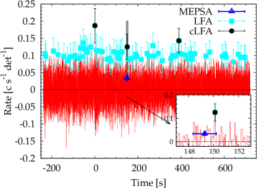
As an illustrative example Figure 1 shows a group–2 light curve together with the FPs identified by each algorithm. MEPSA has the lowest FP rate, $\sim 1$–$2\times 10^{-5}$ FP/bin, which is equivalent to a $4.2$–$4.4\,\sigma$ (Gaussian) significance threshold. cLFA has a significantly worse FP rate, about 4–5 times as high, corresponding to $3.9$–$4.0\,\sigma$ (Gaussian), whereas LFA is by far the worst, with a rate of $3$–$5\times 10^{-3}$ FP/bin, corresponding to $2.8$–$2.9\,\sigma$ (Gaussian). The ratio between LFA and cLFA significance Gaussian thresholds is indeed compatible with $\sqrt{2}$, as expected (Sect. 2.1).

Figure 2: MEPSA FP (dashed) and TP (solid) spectra, i.e., number of events as a function of the triggering pattern. The TP spectrum has been downsized so as to have the same area as the FP one.

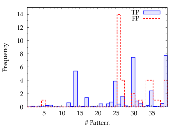
In the case of MEPSA, we also studied the FP rate as a function of the triggering pattern through what can be considered as a “FP spectrum”. The dashed histogram in Figure 2 shows how the 36 FPs detected in group 2 profiles distribute among the 39 patterns. Clearly, pattern 26 has the highest FP rate and thus appears to be the weakest pattern in this respect. The FP spectrum is compared with the TP one obtained from the simulated peaks described in Sect. 3.2.

Figure 3: Peak detection efficiency in the SNR–separability plane for MEPSA (left), LFA (mid), and cLFA (right). Different Contour levels (from cold to hot colours) correspond to ten different, equally spaced efficiency levels from 0% to 100% with increasing order. The MEPSA 90% contour level is approximately described with two connected power-laws (dashed line) and is shown in all panels for comparison. Dots and background colours represent the bivariate distribution of the detected peaks.

3.2 True Positive rate

Starting from the same template of Swift/BAT mask–weighted background time profile used to build group 2, we simulated 150 curves populated with fast–rise exponential decay (FRED) pulses assuming the model by Norris et al. (1996). We assumed a fixed value for the peakedness given by the average value found in real GRBs, $\nu=1.5$ (Norris et al., 1996). This corresponds to a pulse shape which lies between a pure exponential and a Gaussian profile. We also assumed fixed rise and decays times, $\sigma_{\rm r}=1$ and $\sigma_{\rm d}=3$ s, respectively, in agreement with what is typically observed in GRB time profiles (Norris et al., 1996). In this mathematical formulation, the corresponding full width at half maximum (hereafter, FWHM) amounts to $(\ln{2})^{1/\nu}\,(\sigma_{\rm r}+\sigma_{\rm d})$.

As will be shown in the following, the relevant parameter for the peak detection of a given pulse is the ratio between its lowest adjacent waiting time $\Delta t_{\rm min}$ and its FWHM, rather than the absolute value of the FWHM itself. For a given $i$–th pulse peaking at $t_{{\rm p},i}$, the lowest adjacent waiting time is defined as $\Delta t_{{\rm min},i}={\rm min}(t_{{\rm p},i}-t_{{\rm p},i-1},t_{{\rm p},i+1}-t_{{\rm p},i})$. This explains our choice of adopting a fixed FWHM for the simulated pulses, since we varied the waiting time distribution. The higher the ratio, the more easily the pulse can be recognised as a separate entity from its surrounding siblings. We therefore define the separability $s_{i}$ of a given pulse $i$, as

$$s_{i}=\frac{\Delta t_{{\rm min},i}}{{\rm FWHM}_{i}}\;.$$ (2)

The more two adjacent pulses overlap, the lower their individual separabilities, and correspondingly harder for a given algorithm is to identify them as two separate entities. The peakedness, which determines the shape of the pulse profile, is expected to have a minor weight as far as the peak detection is concerned, provided that extreme and nonphysical values are not considered. This justifies our choice of assuming a typical, fixed value for it, and our choice of exploring more in detail the effects of other more crucial parameters, such as the SNR of the pulse, i.e. the ratio between the total area (or fluence) and its statistical uncertainty, and the ratio between the time intervals mentioned above.

Different pulses within the same simulated curve were generated assuming an exponential distribution for the waiting times, i.e. the case of a memoryless process with a constant expected Poisson rate of pulses per unit time. We assumed a range for the expected rates of pulses from $1/40$ up to $1/20$ pulses s^-1. Peak intensities were assumed so as to cover the SNR range from $2$ all the way up to $100$. The nature of the waiting time distribution (an exponential in this case) is not relevant to our goal; rather, the aim is covering as much as possible the SNR–separability plane and monitoring the algorithms’ efficiency as a function of both variates.

Overall, $89\,540$ pulses were generated spanning the ranges $0.5\lesssim\log{({\rm SNR})}\lesssim 2.0$ and $-3\lesssim\log{s}\lesssim 2$.

3.2.1 Efficiency

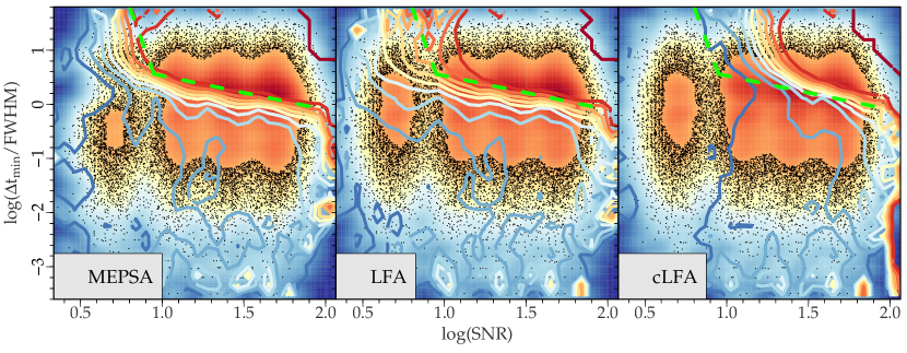
We split the SNR–$s$ plane in 30 different boxes and for each of them we calculated the fraction of identified peaks over the total number of pulses. Left–hand panel in Figure 3 shows the MEPSA efficiency. The 90% contour level can approximately be described with a double piece-wise power–law (dashed line in Fig. 3), whose equation is

$$\log{s_{0.9}({\rm SNR})}=\left\{\begin{array}[]{lr}-8.28\,\log{({\rm SNR})}+8.42&(\log{({\rm SNR})<0.95})\\ -0.63\,\log{({\rm SNR})}+1.15&(\log{({\rm SNR})\geq 0.95})\end{array}\right.\;.$$ (3)

Figure 4: Left panel: MEPSA estimated vs. true peak rates for weakly separated ($1<s<10$, grey) and well separated pulses ($s>10$, red). The solid line shows equality. Right panel: corresponding violin plot of normalised residuals of estimated vs. true values for different classes of SNR of well separated pulses.

Whenever the condition $s({\rm SNR})\geq s_{0.9}({\rm SNR})$ is fulfilled, MEPSA efficiency is 90% at least. Worth noting are the following properties:

• efficiency is very high in the top right region of well separated, high contrast pulses, as one expects;

• when $\log{s}<-0.4$, i.e. $s<0.4$, pulses can hardly ($<$10–20%) be identified as separate pulses, regardless of the SNR;

• at a given separability, efficiency slightly improves for higher SNR;

• when SNR drops below 4–5, efficiency drops as well almost regardless of separability;

• at fixed SNR$>$4–5, efficiency drops from 90% to 50% when separability decreases from $s_{0.9}$(SNR) by a factor of $\sim 10^{-0.2}\approx 0.6$.

Likewise, we studied of efficiency in the SNR–$s$ plane for the other two algorithms. Mid and right–hand panels in Figure 3 show the results for LFA and cLFA, respectively: the dashed line in both plots is the same as in right–hand panel and described by Eq. (3) for comparison. At given separability values, LFA has comparable efficiency values as long as SNR$\gtrsim 15$. However, at SNR $<15$ LFA efficiency becomes remarkably worse than MEPSA (e.g., 60% vs. 90%, at SNR $\sim 8$ and $s>3$). This proves that MEPSA has a higher TP (lower TN) rate than LFA in low-intermediate SNR range, i.e. 4–5 $<$ SNR $<$ 15.

Compared with MEPSA and LFA, the TP rate of cLFA is the lowest (highest TN rate), since the $>90$% efficiency region shrinks along both SNR and $s$, as shown in the right–hand panel of Fig. 3. This is no wonder, because it is the downside of a relatively low FP rate, typical of a more selective algorithm.

3.2.2 Accuracy of peak rate estimates

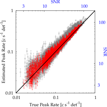
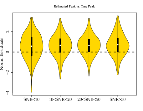
We investigated the accuracy of different algorithms in estimating peak intensities or rates, something that can be done only for the TP peaks. Left–hand panel of Figure 4 shows MEPSA–estimated vs. true peak rates for two different classes of separability $s$: the mildly separated pulses ($1<s<10$, grey), and the well separated ones ($s>10$, red). The mildly separated peak rates tend to scatter more significantly above equality than well separated ones do: the reason behind this is that more overlapping pulses are more likely to be identified as a single peak, whose estimated rate is therefore the sum of different pulses’ contributions. While the scatter around equality seems to enhance in the low–SNR (or low–rate) end of the distribution, the corresponding uncertainties increase as well. To better understand whether the accuracy of a MEPSA–estimated peak rate depends on SNR or, equivalently, on the value of the rate itself, we show in the right–hand panel of Fig. 4 the violin plot of the normalised scatter, i.e. the difference between true and estimated values normalised by the estimated uncertainty, as a function of peak rate. We considered the sample of well separated pulses ($s>10$) only. There is no significant trend with peak rate: the variance of distribution remains essentially unchanged throughout the spanned range, and so does the mean value. In all cases the null value is within $1\,\sigma$ of the distribution. All mean values are above zero, suggestive of a small bias that tends to overestimates the peak rate, even though it is still within uncertainties. A possible explanation for that is that MEPSA searches the peak through all the possible binnings and shifts, with the result of a slight bias towards positive statistical fluctuations.

Figure 5 shows the analogous violin plots for the normalised residuals for LFA and cFLA, respectively, for the identified well separated pulses. In both cases, the accuracy is remarkably worse at low SNR values, where peak rate estimates become crucially biased by statistical fluctuations that overestimate as much as up to $\sim 3\,\sigma$. It is worth noting that in this respect cLFA is even worse on average.

Figure 5: Violin plots of the normalised residuals for both versions of LF algorithms: LFA (top) and cLFA (bottom), analogously to Fig. 4. Both LFA and cLFA provide significantly more biased estimates of the true peak rates than our algorithm does.

3.2.3 MEPSA proxy for the peak FWHM

Both MEPSA and LFA algorithms do not assume any specific shape for the peaks. As non–parametric methods, they have the benefit of being applicable to a broad variety of time series characterised by peaks. The downside is that peak FWHM must be estimated from the data themselves and not through fitting parameters that are linked to specific peak models. LFA algorithms provide no direct information about peak width, the only bare proxy being the times of the two adjacent valleys surrounding a given peak.

Analogously, a detection timescale $\Delta t_{\rm det}$ is associated to each MEPSA peak (Sect. 2). As in the case of LFA valleys, the detection timescale is affected by the peak SNR: at low SNR values it tends to bin up the light curve as much as possible to reach the required statistical excess to trigger MEPSA. On the other side, at high SNR the peak already triggers some MEPSA patterns at low timescales and at longer timescale, although the SNR increases, the average peak rate estimate likely decreases. All this turns into favouring the short timescales at high SNR and the other way around at low SNR. This is indeed what is observed when one studies the distribution of the ratio between detection timescale and FWHM for three different SNR ranges, as shown by Fig. 6.

Figure 6: Distribution of the ratio between MEPSA detection timescale $\Delta t_{\rm det}$, used as a proxy for the pulse FWHM, and the FWHM itself. This is done separately for different SNR classes.

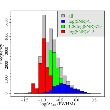
Looking at the mean values and scatters of each distribution, we conclude that, on average,

• at $\log{({\rm SNR})}>1.5$, it is FWHM$\approx 10\,\Delta_{\rm det}$,

• at $1.0<\log{({\rm SNR})}<1.5$, it is FWHM$\approx 5-6\,\Delta_{\rm det}$,

• at $\log{({\rm SNR})}<1.0$, it is FWHM$\approx 2.5\,\Delta_{\rm det}$,

with a factor of $\approx$2–3 uncertainty.

3.2.4 MEPSA proxy for the peak SNR

Similarly to peak FWHM discussed in Sect. 3.2.3, MEPSA does not provide a direct estimate of the peak SNR, to calculate which one should integrate over the entire pulse profile or, equivalently, over its FWHM and correct it by a given factor. As it was shown in Sect. 3.2.3, MEPSA can only roughly estimate the FWHM, and so does it for the SNR, too. A SNR proxy is yielded by the estimated SNR, SNR_est, which is calculated by MEPSA over the detection time $\Delta t_{\rm det}$.

We studied the relation between the estimated and true SNR’s for the sample of well separated simulated peaks and obtained that, regardless of the scatter, the relation can be approximately linearly described as,

$${\rm SNR}_{\rm est}\ \approx\ 0.29\,{\rm SNR}+3.9\;,$$ (4)

as displayed by Figure 7.

Figure 7: Relation between estimated and true SNR for a sample of well separated ($s>10$) peaks that have been identified by MEPSA.

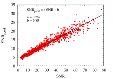
Practically, starting from the values obtained by MEPSA for the SNR_est and $\Delta t_{\rm det}$ of a given peak, one could use Eq. (4) to estimate the true SNR, and use it to roughly estimate its FWHM using the approximate relations of Sect. 3.2.3. This, in turn, allows one to place the peak in the separability–FWHM plane shown in left–hand panel of Fig. 3 and estimate the efficiency–corrected rate of such peaks in the time series.

4 Discussion and Conclusions

We presented MEPSA, multiple excess peak search algorithm, which searches for peaks by applying a mask of multi–excess patterns to an evenly spaced, background–subtracted (or detrended) time series, which is thought to be affected by statistical uncorrelated Gaussian noise. This is often the case also for photon counting detectors operating in the high counting regime. We compared its performance against the popular and widely adopted LFA as well as with a slightly more conservative version of the same, under two complementary aspects: the false positive and the true positive rates. In either case MEPSA is more reliable, showing a lower FP rate ($\lesssim 2\times 10^{-5}$ bin^-1) as well as a higher true positive one, especially at low SNR ($\sim$ 4–5). We showed that MEPSA efficiency most crucially depends on the combination of separability, defined as the ratio between the lowest temporal separation from adjacent peaks and the FWHM of a given peak, and SNR. At SNR$<$4–5, efficiency significantly drops. This is also the case when adjacent peaks overlap non–negligibly, i.e. when separability drops below 1, with little but significant dependence on SNR, that we modelled with a double power–law in the separability–SNR plane. MEPSA also yields some proxies to characterise FWHM and SNR of pulses and we described a quick way to do that.

Although the motivation originally sprang up from GRB time profiles, its applicability extends to other similar fields of high–energy astrophysics as well as solar X–ray flares, and, more in general, whenever the applicability requirements on the input time series are fulfilled. The search algorithm is decoupled from the mask of multiple excesses being searched. This property makes it particularly flexible, so that users possibly interested in events other than GRBs can quickly modify and optimise the mask of multiple excesses, disable existing patterns and/or enable new ones, once these have been tested through simulations or independent data sets. The highly–portable C code is made publicly available so as to encourage a broad optimisation through other kinds of astrophysical time series of interest.

Appendix A Information provided by MEPSA

This section presents the information provided by MEPSA for each peak candidate. Table 3 shows an example. Field names and header line are the same as what is printed to standard output by MEPSA.

Table 3: Information provided by MEPSA. Each line refers to each peak candidate.

Peak	RebF	BinPhase	PeakT	BinT	PeakR	EPeakR	SNR	Criterium	Nadiac
1	35	34	-12.408	2.240	0.04405	0.00612	7.20	25	9
2	11	6	1.800	0.704	0.07064	0.01129	6.25	30	10

1. Peak: ordinal number of the peak candidate;

2. RebF: rebinning factor chosen by MEPSA of the original time series for the peak candidate;

3. BinPhase: binning phase (from 0 to RebF$-1$) chosen by MEPSA;

4. PeakT: peak time;

5. BinT: detection timescale, $\Delta t_{\rm det}$, which is given by the original time resolution of the time series multiplied by RebF;

6. PeakR: peak rate estimate (same units as the original time series);

7. EPeakR: error on PeakR;

8. SNR: SNR_est;

9. Criterium: triggered pattern (Sect. 2);

10. Nadiac: number of adjacent bins involved in the triggered pattern identified by Criterium.

References

- Bhat et al. (2012) Bhat, P. N., Briggs, M. S., Connaughton, V., Kouveliotou, C., van der Horst, A. J., Paciesas, W., Meegan, C. A., Bissaldi, E., Burgess, M., Chaplin, V., Diehl, R., Fishman, G., Fitzpatrick, G., Foley, S., Gibby, M., Giles, M. M., Goldstein, A., Greiner, J., Gruber, D., Guiriec, S., von Kienlin, A., Kippen, M., McBreen, S., Preece, R., Rau, A., Tierney, D., Wilson-Hodge, C., Jan. 2012. Temporal Deconvolution Study of Long and Short Gamma-Ray Burst Light Curves. ApJ 744, 141.
- Charisi et al. (2014) Charisi, M., Márka, S., Bartos, I., Sep. 2014. Catalog of Isolated Emission Episodes in Gamma-ray Bursts From Fermi, Swift and BATSE. in press, arXiv 1409.2491.
- Drago and Pagliara (2007) Drago, A., Pagliara, G., Aug. 2007. Quiescent Times in Gamma-Ray Bursts: Hints of a Dormant Inner Engine. ApJ 665, 1227–1234.
- Feng et al. (1999) Feng, Y. X., Li, T. P., Chen, L., Mar. 1999. X-Ray Shots of Cygnus X-1. ApJ 514, 373–382.
- Frontera et al. (2009) Frontera, F., Guidorzi, C., Montanari, E., Rossi, F., Costa, E., Feroci, M., Calura, F., Rapisarda, M., Amati, L., Carturan, D., Cinti, M. R., Fiume, D. D., Nicastro, L., Orlandini, M., Jan. 2009. The Gamma-Ray Burst Catalog Obtained with the Gamma-Ray Burst Monitor Aboard BeppoSAX. ApJS 180, 192–223.
- Greco et al. (2011) Greco, G., Rosa, R., Beskin, G., Karpov, S., Romano, L., Guarnieri, A., Bartolini, C., Bedogni, R., Sep. 2011. Evidence of Deterministic Components in the Apparent Randomness of GRBs: Clues of a Chaotic Dynamic. Nature Scientific Reports 1.
- Horváth et al. (2010) Horváth, I., Bagoly, Z., Balázs, L. G., de Ugarte Postigo, A., Veres, P., Mészáros, A., Apr. 2010. Detailed Classification of Swift ’s Gamma-ray Bursts. ApJ 713, 552–557.
- Kouveliotou et al. (1993) Kouveliotou, C., Meegan, C. A., Fishman, G. J., Bhat, N. P., Briggs, M. S., Koshut, T. M., Paciesas, W. S., Pendleton, G. N., Aug. 1993. Identification of two classes of gamma-ray bursts. ApJ 413, L101–L104.
- Krimm et al. (2010) Krimm, H. A., Barthelmy, S. D., Baumgartner, W. H., Beardmore, A. P., Cummings, J. R., Fenimore, E. E., Gehrels, N., Markwardt, C. B., Palmer, D. M., Parsons, A. M., Sakamoto, T., Sato, G., Stamatikos, M., Tueller, J., Ukwatta, T. N., 2010. GRB 100814A, Swift-BAT refined analysis. GRB Coordinates Network 11094, 1.
- Kumar and Zhang (2014) Kumar, P., Zhang, B., Oct. 2014. The Physics of Gamma-Ray Bursts and Relativistic Jets. in press to Phys. Rep., arXiv 1410.0679.
- Levan et al. (2014) Levan, A. J., Tanvir, N. R., Starling, R. L. C., Wiersema, K., Page, K. L., Perley, D. A., Schulze, S., Wynn, G. A., Chornock, R., Hjorth, J., Cenko, S. B., Fruchter, A. S., O’Brien, P. T., Brown, G. C., Tunnicliffe, R. L., Malesani, D., Jakobsson, P., Watson, D., Berger, E., Bersier, D., Cobb, B. E., Covino, S., Cucchiara, A., de Ugarte Postigo, A., Fox, D. B., Gal-Yam, A., Goldoni, P., Gorosabel, J., Kaper, L., Krühler, T., Karjalainen, R., Osborne, J. P., Pian, E., Sánchez-Ramírez, R., Schmidt, B., Skillen, I., Tagliaferri, G., Thöne, C., Vaduvescu, O., Wijers, R. A. M. J., Zauderer, B. A., Jan. 2014. A New Population of Ultra-long Duration Gamma-Ray Bursts. ApJ 781, 13.
- Li and Fenimore (1996) Li, H., Fenimore, E. E., Oct. 1996. Log-normal Distributions in Gamma-Ray Burst Time Histories. ApJ 469, L115.
- Liu and Li (2004) Liu, C. Z., Li, T. P., Aug. 2004. X-Ray Spectral Variability in Cygnus X-1. ApJ 611, 1084–1090.
- Margutti et al. (2011) Margutti, R., Guidorzi, C., Chincarini, G., 2011. Variability Properties of Swift-Bat Gamma-Ray Bursts. International Journal of Modern Physics D 20, 1969–1973.
- Mereghetti (2008) Mereghetti, S., Jul. 2008. The strongest cosmic magnets: soft gamma-ray repeaters and anomalous X-ray pulsars. A&ARv 15, 225–287.
- Nakar and Piran (2002) Nakar, E., Piran, T., Mar. 2002. Time-scales in long gamma-ray bursts. MNRAS 331, 40–44.
- Norris et al. (1996) Norris, J. P., Nemiroff, R. J., Bonnell, J. T., Scargle, J. D., Kouveliotou, C., Paciesas, W. S., Meegan, C. A., Fishman, G. J., Mar. 1996. Attributes of Pulses in Long Bright Gamma-Ray Bursts. ApJ 459, 393.
- Paciesas et al. (1999) Paciesas, W. S., Meegan, C. A., Pendleton, G. N., Briggs, M. S., Kouveliotou, C., Koshut, T. M., Lestrade, J. P., McCollough, M. L., Brainerd, J. J., Hakkila, J., Henze, W., Preece, R. D., Connaughton, V., Kippen, R. M., Mallozzi, R. S., Fishman, G. J., Richardson, G. A., Sahi, M., Jun. 1999. The Fourth BATSE Gamma-Ray Burst Catalog (Revised). ApJS 122, 465–495.
- Quilligan et al. (2002) Quilligan, F., McBreen, B., Hanlon, L., McBreen, S., Hurley, K. J., Watson, D., Apr. 2002. Temporal properties of gamma ray bursts as signatures of jets from the central engine. A&A 385, 377–398.
- Remillard and McClintock (2006) Remillard, R. A., McClintock, J. E., Sep. 2006. X-Ray Properties of Black-Hole Binaries. ARAA 44, 49–92.
- Romano et al. (2014) Romano, P., Krimm, H. A., Palmer, D. M., Ducci, L., Esposito, P., Vercellone, S., Evans, P. A., Guidorzi, C., Mangano, V., Kennea, J. A., Barthelmy, S. D., Burrows, D. N., Gehrels, N., Feb. 2014. The 100-month Swift catalogue of supergiant fast X-ray transients. I. BAT on-board and transient monitor flares. A&A 562, A2.
- Sakamoto et al. (2011) Sakamoto, T., Barthelmy, S. D., Baumgartner, W. H., Cummings, J. R., Fenimore, E. E., Gehrels, N., Krimm, H. A., Markwardt, C. B., Palmer, D. M., Parsons, A. M., Sato, G., Stamatikos, M., Tueller, J., Ukwatta, T. N., Zhang, B., Jul. 2011. The Second Swift Burst Alert Telescope Gamma-Ray Burst Catalog. ApJS 195, 2.
- Sguera et al. (2005) Sguera, V., Barlow, E. J., Bird, A. J., Clark, D. J., Dean, A. J., Hill, A. B., Moran, L., Shaw, S. E., Willis, D. R., Bazzano, A., Ubertini, P., Malizia, A., Dec. 2005. INTEGRAL observations of recurrent fast X-ray transient sources. A&A 444, 221–231.