Charge ordering and self-assembled nanostructures in a fcc Coulomb lattice gas

Abstract

The compositional ordering of Ag, Pb, Sb, Te ions in (AgSbTe₂)_x(PbTe)_2(1-x) systems possessing a NaCl structure is studied using a Coulomb lattice gas (CLG) model on a face-centered cubic (fcc) lattice and Monte Carlo simulations. Our results show different possible microstructural orderings. Ordered superlattice structures formed out of AgSbTe₂ layers separated by Pb₂Te₂ layers are observed for a large range of $x$ values. For $x=0.5$, we see an array of tubular structures formed by AgSbTe₂ and Pb₂Te₂ blocks. For $x=1$, AgSbTe₂ has a body-centered tetragonal (bct) structure which is in agreement with previous Monte Carlo simulation results for restricted primitive model (RPM) at closed packed density. The phase diagram of this frustrated CLG system is discussed.

I Introduction

Lattice gas with long-range Coulomb interaction has attracted considerable interest over the past 10 years. Two types of long-range models have been studied. One where the interaction between the charges $\propto 1/r$ (Coulomb lattice gas, or CLG), and the other where the interaction $\propto\ln r$ (lattice Coulomb gas, or LCG). Studies of various models of oneking1 ; king2 ; king3 ; levashov - and twolevashov ; teitel1 ; teitel2 -dimensional CLG and LCG using different methods have shown the existence of multiple phase transitions, complexity in phase diagrams and their practical applications to real materials, e.g., KCu_7-xS${}_{4},$king1 ; king2 ; king3 Ni_1-xAl_x(OH)₂(CO₃)_x/2.$y$H₂O,… .levashov In three-dimensional CLG on a simple cubic (sc) lattice, several works have been done using either theoretical calculations (mean-field approximationstell and Padé expansionwalker ) or Monte Carlo (MC) simulations.stell ; van However, to the best of our knowledge, there are no extensive studies of CLG on a fcc lattice excepting when all the lattice sites are occupied by either a positive or a negative charge.bresme It is well known that fcc lattice involves frustration.toulouse Since the role played by frustration in the nature of phase transition in Ising-type systems (on triangular or fcc lattice) has been of great interest in statistical physics,wannier ; alexander ; heilmann ; phani ; kammerer it is of equal interest to see what role frustration effects play in long-range Coulomb systems.

From materials perspective, a quaternary compound Ag_nPb_mSb_nTe_m+2n has recently emerged as a material for potential use in efficient thermoelectric power generation. It has been found that for low concentrations of Ag, Sb and when doped appropriately, this system exhibits a high thermoelectric figure of merit $ZT$ of $\approx$2.2 at 800 K.hsu It is one of the best known bulk thermoelectrics at high temperatures. Quantitative understanding of its properties requires understanding of atomic structure. Experimental datahsu ; eric suggest that this system belongs to an entire family of compounds, which are compositionally complex yet they possess the simple cubic NaCl structure on average, but the detailed ordering of Ag, Pb and Sb ions is not clear. However, as pointed out by Bilc et al.,bilc the electronic structure of these compounds depends sensitively on the nature of structural arrangements of Ag and Sb ions. Hence a simple but accurate theoretical model is necessary to understand and predict the ordering of the ions in these systems. In this paper we present a simple ionic model of Ag_nPb_mSb_nTe_m+2n that explicitly includes the long-range Coulomb interaction and in which the ions are located at the sites of a fcc lattice. As will be shown in the next section, this problem maps onto a spin-$1$ Ising model on a fcc lattice with long-range antiferromagnetic interaction. We present details of the model in Sec. II. In Sec. III we discuss our Monte Carlo simulation results including a full phase diagram in the $x-T$ plane. The summary is presented in Sec. IV.

II Model

We use a model where the minimization of electrostatic interaction between different ions in the compounds can lead to the compositional ordering that exists in the system.hsu The total electrostatic energy is then expressed as

$$E=\frac{e^{2}}{2}\sum_{l\tau\neq l^{{}^{\prime}}\tau^{{}^{\prime}}}\frac{Q_{l\tau}Q_{l^{{}^{\prime}}\tau^{{}^{\prime}}}}{\epsilon\mid\mathbf{R}_{l\tau}-\mathbf{R}_{l^{{}^{\prime}}\tau^{{}^{\prime}}}\mid}\,,$$ (1)

where $\epsilon$ is the static dielectric constant, $\mathbf{R}_{l\tau}$ and $Q_{l\tau}$ are, respectively, the position and charge of an atom at site $\tau$ of cell $l$. This model has been successfully applied to cubic perovskite alloys. van Here we consider supercells of the NaCl-type structure made of two interpenetrating fcc lattices with possible mixtures of different atomic species on Na sites, i.e., $\tau=\{$Na(Ag,Sb,Pb), Cl(Te)$\}$, with periodic boundary condition. Alloying occurs on the Na sublattice. In a simple ionic model of Ag_nPb_mSb_nTe_m+2n, we can assume the Pb ion to be $2^{+}$, Te ion to be $2^{-}$, Ag ion to be $1^{+}$, and Sb ion to be $3^{+}$, i.e., $Q_{l\tau}=\{Q_{l,\mathrm{Na}};Q_{l,\mathrm{Cl}}\}=\{+1,+3,+2;-2\}$, where $Q_{l,\mathrm{Cl}}=q_{\mathrm{Cl}}=-2$ is independent of $l$. Focusing on the Na sublattice sites where ordering occurs, we write $Q_{l\tau,\mathrm{Na}}=q_{\mathrm{Na}}+\Delta q_{l}$, where $q_{\mathrm{Na}}=+2$ and $\Delta q_{l}=\{-1,+1,0\}$. Substituting the expression for $Q_{l,\mathrm{Na}}$ into Eq. (1), we can write $E=E_{0}+E_{1}+E_{2}$, where the subscripts refer to the number of powers of $\Delta q_{l}$ appearing in that term. Then $E_{0}$ is just a constant, it is the energy of an ideal PbTe lattice; $E_{1}$ vanishes due to charge neutrality. The only term which depends on the charge configuration is $E_{2}$; it is given by

$$E_{2}=\frac{e^{2}}{2\epsilon a}\sum_{l\neq l^{{}^{\prime}}}\frac{\Delta q_{l}\Delta q_{l^{{}^{\prime}}}}{\mid\mathbf{l}-\mathbf{l^{{}^{\prime}}}\mid}\equiv\frac{J}{2}\sum_{l\neq l^{{}^{\prime}}}\frac{s_{l}s_{l^{{}^{\prime}}}}{\mid\mathbf{l}-\mathbf{l^{{}^{\prime}}}\mid}\,,$$ (2)

where ion positions are measured in unit of the fcc lattice constant $a$; $l$ and $l^{{}^{\prime}}$ run over the $N$ sites of the Na-sublattice of NaCl structure. Thus if we start from a PbTe lattice as a reference system and replace two Pb ions by one Ag ion and one Sb ion, we map the system unto an effective CLG with effective charges -1, +1 (of equal amount) and 0; this implies a constraint, $\sum_{l}\Delta q_{l}=0$. The model therefore maps onto a spin-$1$ Ising model ($s_{l}=0,\pm 1$) with long-range antiferromagnetic interaction. The short-range version of this model [nearest- (n.n.) and next-nearest-neighbor (n.n.n.) interaction],heilmann ; phani ; kammerer a generalization of this model by adding a n.n ferromagnetic interactiongrousson and a continuum version of this model that takes into account the finite size of the charged particles (RPM or charged hard sphere model)stellwu ; orkoulas ; pana ; bresme ; kobelev ; ciach have been investigated. Comparison with these works will be made in Sec. III.

Because of the attraction between +1 and -1 charges, the Ag and Sb ions tend to come together and form clusters or some sort of ordered structures depending on the temperature at which these compounds are synthesized and the annealing scheme. The ordering may be quite complex compared to the one on a simple cubic lattice because of the frustration associated with spins on a fcc lattice and antiferromagnetic interaction (in the Ising model). In our calculations of Ag_nPb_mSb_nTe_m+2n, an equivalent formula, (AgSbTe₂)_x(PbTe)_2(1-x), is used; where $x=2n/(m+2n)=1/N\sum_{l}|\Delta q_{l}|\equiv 1/N\sum_{l}s_{l}^{2}$ ($0\leq x\leq 1$), is the concentration of Ag and Sb in the Pb sublattice.

III Simulation Results

To study the thermodynamic properties and microstructural ordering of the system, we have done canonical ensemble Monte Carlo simulations following the usual Metropolis criterion metro using the energy given by Eq. (2), i.e., particles interact via site-exclusive (multiple occupancy forbidden) Coulomb interaction. In the Ising model problem, this corresponds to a fixed magnetization simulation. We used Ewald summation ewald to handle this long-range interaction employing a very fast lookup table scheme using Hoshen-Kopelman algorithm.hk This model is parameter-free in the sense that $J=e^{2}/\epsilon a$ defines a characteristic energy.

A simulation for a fixed concentration $x$ starts at a high temperature with an initial random configuration followed by gradual cooling. For each temperature $T$, we use $2\times 10^{4}$ sweeps (MC steps per lattice site) to get thermal equilibration followed by $10^{5}$ sweeps for averaging. Particles move either via hopping to empty sites or via exchange mechanism. The equilibrium configuration at a given temperature $T$ is used as the initial configuration for a study at a nearby temperature. We monitored different thermodynamic quantities and look at the microstructures. The data presented below were obtained with system size $L=8$ (i.e., $8$ fcc cells in one direction, 2048 lattice sites in total) with periodic boundaries.

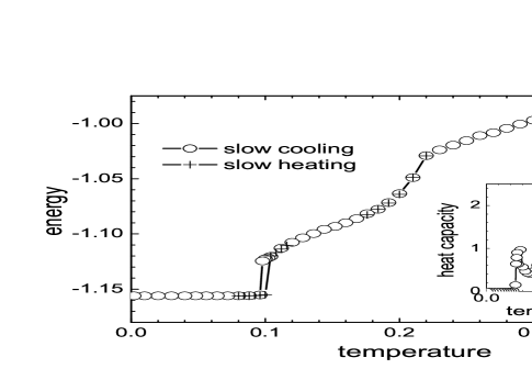
Figure 1: Energy and heat capacity per particle versus temperature for $x=0.75$. Phase transitions occur at $T=0.106$ and $0.21$ which are first-order and second-order transitions, respectively. There is hysteresis associated with the low $T$ transition.

Figure 1 shows the energy and heat capacity (obtained using energy fluctuation) for $x=0.75$ where the two energy curves correspond to slow cooling and slow heating. We see evidence of two phase transitions, one at $T=0.106$ and the other at $T=0.21$. The heat capacity curve shows peaks at the above two $T$ values. The transition at higher $T$ is continuous and indicates a lattice gas-liquidlike phase transition. There is no apparent hysteresis associated with this transition. The low $T$ transition, on the other hand, appears to be first-order. There is an energy discontinuity and there is hysteresis, albeit small, associated with this transition. For $x\leq 0.5$ we see only one transition which is first-order (Fig. 2).

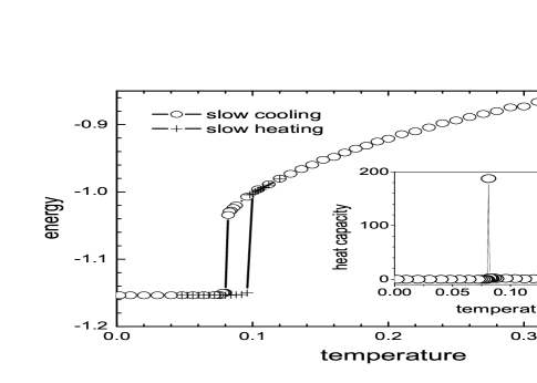
Figure 2: Energy and heat capacity per particle versus temperature for $x=0.25$. Phase transition occurs at $T=0.08$ which is first-order. There is hysteresis associated with this transition.

This suggests that with decreasing $x$ the system changes from undergoing 2 to 1 phase transition. As $x$ decreases from $0.875$, the high $T$ continuous and low $T$ first-order phase transitions approach each other and the two transitions merge at $x\approx 0.5$. As $x$ increases from $0.875$, the high $T$ continuous transition changes to first-order. At $x=1$, the transition is first-order in agreement with previous simulation results.bresme We also monitored the structure factor $S(\mathbf{q})$ for different $\mathbf{q}$ values. For several $\mathbf{q}$ values, we find that $S(\mathbf{q})$ changes discontinuously at the first-order transition and smoothly at a continuous transition.

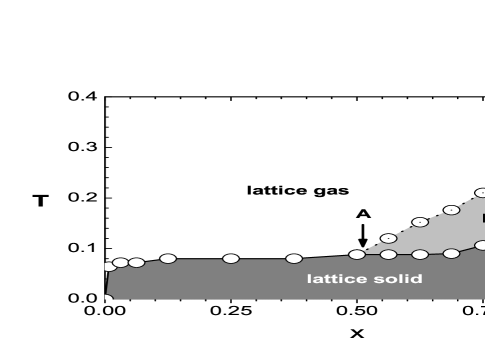
Figure 3: Concentration ($x$) versus temperature ($T$) phase diagram constructed from the loci of the heat capacity maxima. There are first (solid lines) and second (dotted line) order transitions with two possible tricritical points ($x_{t}$, $T_{t}$): A at $\approx(0.500,0.088)$ and B at $\approx(0.875,0.290)$.

To construct the total phase diagram, we have studied energy, heat capacity and structure factor as functions of temperature for a series 15 values of the concentration $x$. Figure 3 shows the phase diagram constructed from the loci of specific heat maxima. The lattice gas-lattice solid and lattice liquid-lattice solid transitions are first-order. In the limit $x=0$, the compound is simply PbTe, the transition occurs at $T=0$ since there are no charged particles (effective charges of Pb and Te are 0). For $x=1$, the compound is AgSbTe₂. Our simulations show a strongly first-order transition at $T=0.38$ and no other transition with decreasing $T$. This strong first-order transition is softened by introducing defects into the system (by decreasing $x$ from 1). The hysteresis associated with this transition becomes smaller with decreasing $x$ from 1 and disappears at $x\approx 0.875$ showing a changeover from a first- to a second-order transition. Therefore, we have two possible tricritical points ($x_{t}$, $T_{t}$): A at $\approx(0.500,0.088)$ and B at $\approx(0.875,0.290)$. More accurate results on the tricritical points would require further careful large-scale simulations for more number of $x$ values, and perhaps much larger systems.

We would now like to compare our results with those of previous simulations carried out for lattice RPM. In this model, there is a parameter $\xi=\sigma/a$, where $\sigma$ is the hard sphere diameter of the charged particles. For $\xi=1$ which is comparable to our model, Dickman and Stellstell and Panagiotopoulos and Kumarpana have a phase diagram for a sc lattice that is similar to ours. They found a tricritical point at ($x_{t}$, $T_{t}$) $\simeq$ ($0.4$, $0.14$) (Ref. 7) and ($0.48\pm 0.02$, $0.15\pm 0.01$).pana It appears that $x_{t}$ values for sc and fcc lattices are quite close whereas the $T_{t}$ values for the fcc lattice is about a factor of 0.6 smaller, perhaps due to frustration. As regards the second tricritical point (B), it is unique to the fcc lattice. Dickman and Stellstell found a high $T$ continuous phase transition ($\lambda$-transition) in a simple cubic lattice as $x$ increased from $0.4$ to $0.82$. The observation of the high $T$ first-order transition in our simulations is similar to the one seen in fully-frustrated n.n. and n.n.n. Ising model ($x=1$) seen by Phani et al.phani

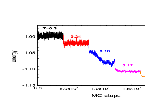
Figure 4: (Color online) Energy as a function of Monte Carlo steps for $x=0.75$. The system is quenched from $T=0.3$ to $0.24$, then from $T=0.24$ to $0.18$, and so on.

In Fig. 4, we plot the energy of a system with $x=0.75$ as a function of Monte Carlo steps as we quench the system from $T=0.3$ to $0.002$ through several intermediate values of $T$. We use more than $4\times 10^{6}$ moves for each $T$ without discarding any step for thermal equilibration. The final configuration at a given $T$ is used as the initial configuration for the next $T$. The fluctuation is large at high $T$ and getting smaller with lowering $T$. From one $T$ to another, it takes some time ($\approx 10^{3}$ steps) for the system to equilibrate. As one crosses the transition region, i.e., from $T=0.24$ to $0.18$ or from $0.12$ to $0.06$, the result shows the existence of possible local minima in energy where the system is in metastable states and then goes to a stable state with lower energy. More details on quenching studies will be reported in another paper.hoang

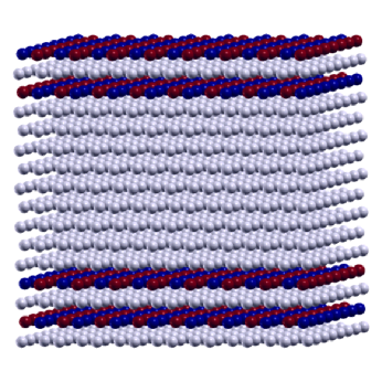
Figure 5: (Color online) A low temperature configuration for $x=0.25$ [created using XCrySDen (Ref. 30)]. Dark layers are for Ag/Sb, grey layers are for Pb; Te sublattice is not shown. This typical configuration showing a ordered superlattice structure formed out of AgSbTe₂ layers separated by Pb₂Te₂ layers.

A typical low temperature structure of (AgSbTe₂)_x(PbTe)_2(1-x) is a self-assembled nanostructure with layers of AgSbTe₂ arranged in a particular fashion in the PbTe bulk as shown in Fig. 5 for the case $x=0.25$. Four layers of AgSbTe₂ are separated from one another by four layers of Pb₂Te₂. This domain is again separated by a purely PbTe domain formed by eight other layers of Pb₂Te₂. Along the $z$-direction (perpendicular to the layers), positive charge and negative charge arrange consecutively. This indicates a three-dimensional long-range order which is clearly a result of the long-range Coulomb interaction. Experimentally, high-resolution transmission electron microscopy (TEM) images indicate inhomogeneities in the microstructure of the materials, showing nano-domains of a Ag-Sb-rich phase embedded in a PbTe matrixhsu ; eric which appears to be consistent with our results. Also electron diffraction measurements show clear experimental evidence of long-range ordering of Ag and Sb ions in AgPb_mSbTe_m+2 (m=18).bilc

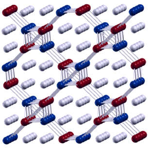
Figure 6: (Color online) A low temperature configuration for $x=0.5$ [created using XCrySDen (Ref. 30)]. Connected balls are for Ag/Sb, unconnected balls are for Pb; Te sub-lattice is not shown. Checkerboard pattern formed by AgSbTe₂ and Pb₂Te₂ blocks.

In addition to the layered superlattice structures seen for several $x$ values, we have also discovered a very interesting structure at $x=0.5$, in which an array of tubes of AgSbTe₂ and Pb₂Te₂ are arranged in a checker board pattern (Fig. 6). We find that this structure has the same energy as the layered structure consisting of alternate layers of AgSbTe₂ and Pb₂Te₂ (energy per particle $E=-1.157278$). For $x=1$, i.e., AgSbTe₂, the only ordered structure is body-centered tetragonal (bct) structure with a $c$-parameter which is double that of the NaCl subcell, belonging to space group $I\overline{4}m2$. The unit cell of this structure has eight ions, with every ion being surrounded by eight ions of opposite charge and four of the same charge (Te sublattice is not included here). This structure is equivalent to the type-III antiferromagnetic structureandersonsmart which has been found in n.n. and n.n.n. Ising model by Phani et al.phani It has also been seen in the RPM by Bresme et al.bresme in Monte Carlo simulations and by Ciach and Stellciach within a field-theoretic approach.

The comparison we made with a system of size $L=4$ shows no appreciable change in the results for the first-order transition except the fact that we did not see any hysteresis with $L=4$. The energy at a given concentration differs by $0.1\%-0.5\%$ from that obtained for $L=8$. However, for the continuous transition along the line joining A and B in Fig. 3, one expects to see the usual finite size effects.landau Most of the earlier simulations have been carried out in systems of similar sizes. For example, the system size $L=4$ was also used by Bresme et al.bresme for a CLG in fcc lattice. Bellaiche and Vanderbiltvan chose $L=6$ for their study of cubic perovskite alloys. For a CLG in sc lattice, larger size lattices have been used because the number of atoms per unit cell is one in this case. For example, Panagiotopoulos and Kumarpana and Dickman and Stellstell chose $L=12$ and $16$, respectively.

IV Summary

In summary, our phase diagram has shown the distinct feature of having two tricritical points for a CLG in fcc lattice. We have demonstrated that Monte Carlo simulation using an ionic model of (AgSbTe₂)_x(PbTe)_2(1-x) shows different possible microstructural orderings. We have found that layered structures formed out of AgSbTe₂ layers separated by Pb₂Te₂ layers are generic low temperature structures. In addition to the layered structures, we have also discovered tubular structures for $x=0.5$. For $x=1$, a bct structure has been found, in agreement with previous simulation results. Structures for other values of $x$ are mixtures of those for $x=0$, $0.5$, and $1$. These results will be discussed in a separate paper.hoang

- (1) T. C. King, Y. K. Kuo, M. J. Skove, and S.-J. Hwu, Phys. Rev. B 63, 045405 (2001).
- (2) T. C. King, Y. K. Kuo, and M. J. Skove, Physica A 313, 427 (2002).
- (3) T. C. King and Y. K. Kuo, Phys. Rev. E 68, 036116 (2003).
- (4) V. Levashov, M. F. Thorpe and B. W. Southern, Phys. Rev. B 67, 224109 (2003).
- (5) J.-R. Lee and S. Teitel, Phys. Rev. B 46, 3247 (1992).
- (6) P. Gupta and S. Teitel, Phys. Rev. B 55, 2756 (1997).
- (7) R. Dickman and G. Stell, in Simulation and Theory of Electrostatic Interactions in Solutions, edited by G. Hummer and L.R. Pratt (AIP, Woodbury, New York, 1999).
- (8) A. B. Walker and M. J. Gillan, J. Phys. C: Solid State Phys. 16, 3025 (1983).
- (9) L. Bellaiche and D. Vanderbilt, Phys. Rev. Lett. 81, 1318 (1998).
- (10) F. Bresme, C. Vega, and J. L. F. Abascal, Phys. Rev. Lett. 85, 3217 (2000).
- (11) G. Toulouse, Commun. Phys. 2, 115 (1977).
- (12) G. H. Wannier, Phys. Rev. 79, 357 (1950); Phys. Rev. B 7, 5017(E) (1973).
- (13) S. Alexander and P. Pincus, J. Phys. A: Math. Gen. 13, 263 (1980).
- (14) O. J. Heilmann, J. Phys. A: Math Gen. 13, 1803 (1980).
- (15) M. K. Phani, J. L. Lebowitz, and M. H. Kalos, Phys. Rev. B 21, 4027 (1980).
- (16) S. Kämmerer, B. Dünweg, K. Binder, and M. d’Onorio de Meo, Phys. Rev. B 53, 2345 (1996).
- (17) K.-F. Hsu, S. Loo, F. Guo, W. Chen, J. S. Dyck, C. Uher, T. Hogan, E. K. Polychroniadis, and M. G. Kanatzidis, Science 303, 818 (2004).
- (18) E. Quarez, K.-F. Hsu, R. Pcionek, N. Frangis, E. K. Polychroniadis, and M. G. Kanatzidis, J. Am. Chem. Soc. 127, 9177 (2005).
- (19) D. Bilc, S. D. Mahanti, K.-F. Hsu, E. Quarez, R. Pcionek, and M. G. Kanatzidis, Phys. Rev. Lett. 93, 146403 (2004).
- (20) M. Grousson, G. Tarjus, and P. Viot, Phys. Rev. E 62, 7781 (2000); 64, 036109 (2001).
- (21) G. Stell, K. C. Wu, and B. Larson, Phys. Rev. Lett. 37, 1369 (1976).
- (22) G. Orkoulas and A. Z. Panagiotopoulos, J. Chem. Phys. 101, 1452 (1994).
- (23) A. Z. Panagiotopoulos and S. K. Kumar, Phys. Rev. Lett. 83, 2981 (1999).
- (24) V. Kolebev, A. B. Kolomeisky, and M. E. Fisher, J. Chem. Phys. 116, 7589 (2002).
- (25) A. Ciach and G. Stell, Phys. Rev. E 70, 016114 (2004).
- (26) N. Metropolis, A. Rosembluth, M. Rosembluth, and A. Teller, J. Chem. Phys. 21, 1087 (1953).
- (27) M. P. Allen and D. J. Tildesley, Computer Simulation of Liquids (Clarendon, Oxford, 1987).
- (28) J. Hoshen and R. Kopelman, Phys. Rev. B 14, 3438 (1976).
- (29) K. Hoang and S. D. Mahanti (in preparation).
- (30) A. Kokalj, J. Mol. Graphics Modelling 17, 176 (1999). Code available from http://www.xcrysden.org/.
- (31) P. W. Anderson, Phys. Rev. 79, 705 (1950); J. S. Smart, ibid. 86, 968 (1952).
- (32) D. P. Landau and K. Binder, A Guide to Monte Carlo Simulations in Statistical Physics (Cambridge University Press, Cambridge, 2000).