The different facets of ice have different hydrophilicities:
Friction at water / ice-I_h interfaces

Abstract

We present evidence that the prismatic and secondary prism facets of ice-I_h crystals possess structural features that can reduce the effective hydrophilicity of the ice/water interface. The spreading dynamics of liquid water droplets on ice facets exhibits long-time behavior that differs for the prismatic $\{10\bar{1}0\}$ and secondary prism $\{11\bar{2}0\}$ facets when compared with the basal $\{0001\}$ and pyramidal $\{20\bar{2}1\}$ facets. We also present the results of simulations of solid-liquid friction of the same four crystal facets being drawn through liquid water, and find that the two prismatic facets exhibit roughly half the solid-liquid friction of the basal and pyramidal facets. These simulations provide evidence that the two prismatic faces have a significantly smaller effective surface area in contact with the liquid water. The ice / water interfacial widths for all four crystal facets are similar (using both structural and dynamic measures), and were found to be independent of the shear rate. Additionally, decomposition of orientational time correlation functions show position-dependence for the short- and longer-time decay components close to the interface.

I Introduction

Surfaces can be characterized as hydrophobic or hydrophilic based on the strength of the interactions with water. Hydrophobic surfaces do not have strong enough interactions with water to overcome the internal attraction between molecules in the liquid phase, and the degree of hydrophilicity of a surface can be described by the extent a droplet can spread out over the surface. The contact angle, $\theta$, formed between the solid and the liquid depends on the free energies of the three interfaces involved, and is given by Young’s equation Young05 ,

$$\cos\theta=(\gamma_{sv}-\gamma_{sl})/\gamma_{lv}.$$ (1)

Here $\gamma_{sv}$, $\gamma_{sl}$, and $\gamma_{lv}$ are the free energies of the solid/vapor, solid/liquid, and liquid/vapor interfaces, respectively. Large contact angles, $\theta>90^{\circ}$, correspond to hydrophobic surfaces with low wettability, while small contact angles, $\theta<90^{\circ}$, correspond to hydrophilic surfaces. Experimentally, measurements of the contact angle of sessile drops is often used to quantify the extent of wetting on surfaces with thermally selective wetting characteristics Tadanaga00 ; Liu04 ; Sun04 .

Nanometer-scale structural features of a solid surface can influence the hydrophilicity to a surprising degree. Small changes in the heights and widths of nano-pillars can change a surface from superhydrophobic, $\theta\geq 150^{\circ}$, to hydrophilic, $\theta\sim 0^{\circ}$ Koishi09 . This is often referred to as the Cassie-Baxter to Wenzel transition. Nano-pillared surfaces with electrically tunable Cassie-Baxter and Wenzel states have also been observed Herbertson06 ; Dhindsa06 ; Verplanck07 ; Ahuja08 ; Manukyan11 . Luzar and coworkers have modeled these transitions on nano-patterned surfaces Daub07 ; Daub10 ; Daub11 ; Ritchie12 , and have found the change in contact angle is due to the field-induced perturbation of hydrogen bonding at the liquid/vapor interface Daub07 .

One would expect the interfaces of ice to be highly hydrophilic (and possibly the most hydrophilic of all solid surfaces). In this paper we present evidence that some of the crystal facets of ice-I_h have structural features that can reduce the effective hydrophilicity. Our evidence for this comes from molecular dynamics (MD) simulations of the spreading dynamics of liquid droplets on these facets, as well as reverse non-equilibrium molecular dynamics (RNEMD) simulations of solid-liquid friction.

Quiescent ice-I_h/water interfaces have been studied extensively using computer simulations. Hayward and Haymet characterized and measured the widths of these interfaces Hayward01 ; Hayward02 . Nada and Furukawa have also modeled the width of basal/water and prismatic/water interfaces Nada95 as well as crystal restructuring at temperatures approaching the melting point Nada00 .

The surface of ice exhibits a pre-melting layer, often called a quasi-liquid layer (QLL), at temperatures near the melting point. MD simulations of the facets of ice-I_h exposed to vacuum have found QLL widths of approximately 10 Å at 3 K below the melting point Conde08 . Similarly, Limmer and Chandler have used the mW water model Molinero09 and statistical field theory to estimate QLL widths at similar temperatures to be about 3 nm Limmer14 .

Recently, Sazaki and Furukawa have developed a technique using laser confocal microscopy combined with differential interference contrast microscopy that has sufficient spatial and temporal resolution to visualize and quantitatively analyze QLLs on ice crystals at temperatures near melting Sazaki10 . They have found the width of the QLLs perpendicular to the surface at -2.2^oC to be 3-4 Å wide. They have also seen the formation of two immiscible QLLs, which displayed different dynamics on the crystal surface Sazaki12 .

Using molecular dynamics simulations, Samadashvili has recently shown that when two smooth ice slabs slide past one another, a stable liquid-like layer develops between them Samadashvili13 . In a previous study, our RNEMD simulations of ice-I_h shearing through liquid water have provided quantitative estimates of the solid-liquid kinetic friction coefficients Louden13 . These displayed a factor of two difference between the basal and prismatic facets. The friction was found to be independent of shear direction relative to the surface orientation. We attributed facet-based difference in liquid-solid friction to the 6.5 Å corrugation of the prismatic face which reduces the effective surface area of the ice that is in direct contact with liquid water.

In the sections that follow, we describe the simulations of droplet-spreading dynamics using standard MD as well as simulations of tribological properties using RNEMD. These simulations give complementary results that point to the prismatic and secondary prism facets having roughly half of their surface area in direct contact with the liquid.

II Methodology

II.1 Construction of the Ice / Water interfaces

Ice I_h crystallizes in the hexagonal space group P$6_{3}/mmc$, and common ice crystals form hexagonal plates with the basal face, $\{0001\}$, forming the top and bottom of each plate, and the prismatic facet, $\{10\bar{1}0\}$, forming the sides. In extreme temperatures or low water saturation conditions, ice crystals can easily form as hollow columns, needles and dendrites. These are structures that expose other crystalline facets of the ice to the surroundings. Among the more common facets are the secondary prism, $\{11\bar{2}0\}$, and pyramidal, $\{20\bar{2}1\}$, faces.

We found it most useful to work with proton-ordered, zero-dipole crystals that expose strips of dangling H-atoms and lone pairs Buch:2008fk . Our structures were created starting from Structure 6 of Hirsch and Ojamäe’s set of orthorhombic representations for ice-I_h Hirsch04 . This crystal structure was cleaved along the four different facets. The exposed face was reoriented normal to the $z$-axis of the simulation cell, and the structures were extended to form large exposed facets in rectangular box geometries. Liquid water boxes were created with identical dimensions (in $x$ and $y$) as the ice, with a $z$ dimension of three times that of the ice block, and a density corresponding to 1 g / cm³. Each of the ice slabs and water boxes were independently equilibrated at a pressure of 1 atm, and the resulting systems were merged by carving out any liquid water molecules within 3 Å of any atoms in the ice slabs. Each of the combined ice/water systems were then equilibrated at 225K, which is the liquid-ice coexistence temperature for SPC/E water Bryk02 . Reference Louden13, contains a more detailed explanation of the construction of similar ice/water interfaces. The resulting dimensions as well as the number of ice and liquid water molecules contained in each of these systems are shown in Table 1.

The SPC/E water model Berendsen87 has been extensively characterized over a wide range of liquid conditions Arbuckle02 ; Kuang12 , and its phase diagram has been well studied Baez95 ; Bryk04b ; Sanz04b ; Fennell:2005fk . With longer cutoff radii and careful treatment of electrostatics, SPC/E mostly avoids metastable crystalline morphologies like ice-i Fennell:2005fk and ice-B Baez95 . The free energies and melting points Baez95 ; Arbuckle02 ; Gay02 ; Bryk02 ; Bryk04b ; Sanz04b ; Fennell:2005fk ; Fernandez06 ; Abascal07 ; Vrbka07 of various other crystalline polymorphs have also been calculated. Haymet et al. have studied quiescent Ice-I_h/water interfaces using the SPC/E water model, and have seen structural and dynamic measurements of the interfacial width that agree well with more expensive water models, although the coexistence temperature for SPC/E is still well below the experimental melting point of real water Bryk02 . Given the extensive data and speed of this model, it is a reasonable choice even though the temperatures required are somewhat lower than real ice / water interfaces.

III Droplet Simulations

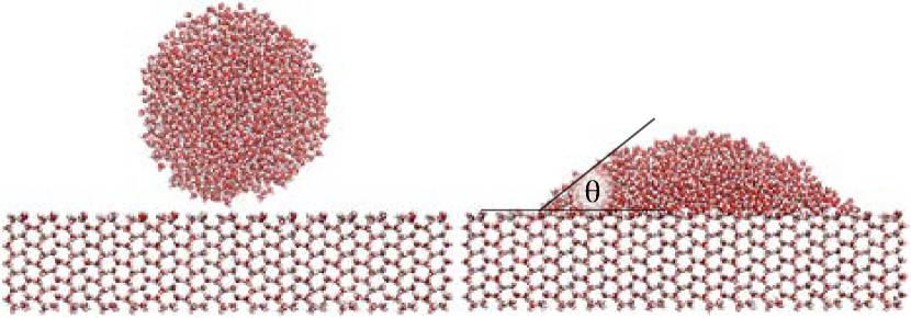
Figure 1: Computational model of a droplet of liquid water spreading over the prismatic $\{10\bar{1}0\}$ facet of ice, before (left) and 2.6 ns after (right) being introduced to the surface. The contact angle ($\theta$) shrinks as the simulation proceeds, and the long-time behavior of this angle is used to estimate the hydrophilicity of the facet.

Ice surfaces with a thickness of $\sim$ 20 Å were created as described above, but were not solvated in a liquid box. The crystals were then replicated along the $x$ and $y$ axes (parallel to the surface) until a large surface ($>$ 126 nm²) had been created. The sizes and numbers of molecules in each of the surfaces is given in Table S1. Weak translational restraining potentials with spring constants of 1.5 $\mathrm{kcal\ mol}^{-1}\mathrm{~{}\AA}^{-2}$ (prismatic and pyramidal facets) or 4.0 $\mathrm{kcal\ mol}^{-1}\mathrm{~{}\AA}^{-2}$ (basal facet) were applied to the centers of mass of each molecule in order to prevent surface melting, although the molecules were allowed to reorient freely. A water droplet containing 2048 SPC/E molecules was created separately. Droplets of this size can produce agreement with the Young contact angle extrapolated to an infinite drop size Daub10 . The surfaces and droplet were independently equilibrated to 225 K, at which time the droplet was placed 3-5 Å above the surface. Five statistically independent simulations were carried out for each facet, and the droplet was placed at unique $x$ and $y$ locations for each of these simulations. Each simulation was 5 ns in length and was conducted in the microcanonical (NVE) ensemble. Representative configurations for the droplet on the prismatic facet are shown in figure 1.

IV Shearing Simulations (Interfaces in Bulk Water)

To perform the shearing simulations, the velocity shearing and scaling variant of reverse non-equilibrium molecular dynamics (VSS-RNEMD) was employed Kuang12 . This method performs a series of simultaneous non-equilibrium exchanges of linear momentum and kinetic energy between two physically-separated regions of the simulation cell. The system responds to this unphysical flux with velocity and temperature gradients. When VSS-RNEMD is applied to bulk liquids, transport properties like the thermal conductivity and the shear viscosity are easily extracted assuming a linear response between the flux and the gradient. At the interfaces between dissimilar materials, the same method can be used to extract interfacial transport properties (e.g. the interfacial thermal conductance and the hydrodynamic slip length).

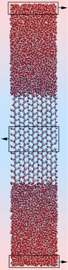
Figure 2: Computational model of a slab of ice being sheared through liquid water. In this figure, the ice is presenting two copies of the prismatic $\{10\bar{1}0\}$ facet towards the liquid phase. The RNEMD simulation exchanges both linear momentum (indicated with arrows) and kinetic energy between the central box and the box that spans the cell boundary. The system responds with weak thermal gradient and a velocity profile that shears the ice relative to the surrounding liquid.

The kinetic energy flux (producing a thermal gradient) is necessary when performing shearing simulations at the ice-water interface in order to prevent the frictional heating due to the shear from melting the crystal. Reference Louden13, provides more details on the VSS-RNEMD method as applied to ice-water interfaces. A representative configuration of the solvated prismatic facet being sheared through liquid water is shown in figure 2.

All simulations were performed using OpenMD OOPSE ; openmd , with a time step of 2 fs and periodic boundary conditions in all three dimensions. Electrostatics were handled using the damped-shifted force real-space electrostatic kernel Ewald .

The interfaces were equilibrated for a total of 10 ns at equilibrium conditions before being exposed to either a shear or thermal gradient. This consisted of 5 ns under a constant temperature (NVT) integrator set to 225 K followed by 5 ns under a microcanonical (NVE) integrator. Weak thermal gradients were allowed to develop using the VSS-RNEMD (NVE) integrator using a small thermal flux ($-2.0\times 10^{-6}$ kcal/mol/Ų/fs) for a duration of 5 ns to allow the gradient to stabilize. The resulting temperature gradient was $\approx$ 10K over the entire box length, which was sufficient to keep the temperature at the interface within $\pm 1$ K of the 225 K target.

Velocity gradients were then imposed using the VSS-RNEMD (NVE) integrator with a range of momentum fluxes. The systems were divided into 100 bins along the $z$-axis for the VSS-RNEMD moves, which were attempted every time step. Although computationally expensive, this was done to minimize the magnitude of each individual momentum exchange. Because individual VSS-RNEMD exchange moves conserve both total energy and linear momentum, the method can be “bolted-on” to simulations in any ensemble. The simulations of the pyramidal interface were performed under the canonical (NVT) ensemble. When time correlation functions were computed, the RNEMD simulations were done in the microcanonical (NVE) ensemble. All simulations of the other interfaces were carried out in the microcanonical ensemble.

These gradients were allowed to stabilize for 1 ns before data collection started. Once established, four successive 0.5 ns runs were performed for each shear rate. During these simulations, configurations of the system were stored every 1 ps, and statistics on the structure and dynamics in each bin were accumulated throughout the simulations. Although there was some small variation in the measured interfacial width between succcessive runs, no indication of bulk melting or crystallization was observed. That is, no large scale changes in the positions of the top and bottom interfaces occurred during the simulations.

V Results

V.1 Ice - Water Contact Angles

To determine the extent of wetting for each of the four crystal facets, contact angles for liquid droplets on the ice surfaces were computed using two methods. In the first method, the droplet is assumed to form a spherical cap, and the contact angle is estimated from the $z$-axis location of the droplet’s center of mass ($z_{\mathrm{cm}}$). This procedure was first described by Hautman and Klein Hautman91 , and was utilized by Hirvi and Pakkanen in their investigation of water droplets on polyethylene and poly(vinyl chloride) surfaces Hirvi06 . For each stored configuration, the contact angle, $\theta$, was found by inverting the expression for the location of the droplet center of mass,

$$\langle z_{\mathrm{cm}}\rangle=2^{-4/3}R_{0}\bigg{(}\frac{1-cos\theta}{2+cos\theta}\bigg{)}^{1/3}\frac{3+cos\theta}{2+cos\theta},$$ (2)

where $R_{0}$ is the radius of the free water droplet.

In addition to the spherical cap method outlined above, a second method for obtaining the contact angle was described by Ruijter, Blake, and Coninck Ruijter99 . This method uses a cylindrical averaging of the droplet’s density profile. A threshold density of 0.5 g cm^-3 is used to estimate the location of the edge of the droplet. The $r$ and $z$-dependence of the droplet’s edge is then fit to a circle, and the contact angle is computed from the intersection of the fit circle with the $z$-axis location of the solid surface. Again, for each stored configuration, the density profile in a set of annular shells was computed. Due to large density fluctuations close to the ice, all shells located within 2 Å of the ice surface were left out of the circular fits. The height of the solid surface ($z_{\mathrm{suface}}$) along with the best fitting origin ($z_{\mathrm{droplet}}$) and radius ($r_{\mathrm{droplet}}$) of the droplet can then be used to compute the contact angle,

$$\theta=90+\frac{180}{\pi}\sin^{-1}\left(\frac{z_{\mathrm{droplet}}-z_{\mathrm{surface}}}{r_{\mathrm{droplet}}}\right).$$ (3)

Both methods provided similar estimates of the dynamic contact angle, although the spherical cap method is significantly less prone to noise, and is the method used to compute the contact angles in table 2.

Because the initial droplet was placed above the surface, the initial value of 180^∘ decayed over time (See figure 1 in the SI). Each of these profiles were fit to a biexponential decay, with a short-time contribution ($\tau_{c}$) that describes the initial contact with the surface, a long time contribution ($\tau_{s}$) that describes the spread of the droplet over the surface, and a constant ($\theta_{\infty}$) to capture the infinite-time estimate of the equilibrium contact angle,

$$\theta(t)=\theta_{\infty}+(180-\theta_{\infty})\left[ae^{-t/\tau_{c}}+(1-a)e^{-t/\tau_{s}}\right]$$ (4)

We have found that the rate for water droplet spreading across all four crystal facets, $k_{\mathrm{spread}}=1/\tau_{s}\approx$ 0.7 ns^-1. However, the basal and pyramidal facets produced estimated equilibrium contact angles, $\theta_{\infty}\approx$ 35^∘, while prismatic and secondary prismatic had values for $\theta_{\infty}$ near 43^∘ as seen in Table 2.

These results indicate that by traditional measures, the basal and pyramidal facets are more hydrophilic than the prismatic and secondary prism facets, and surprisingly, that the differential hydrophilicities of the crystal facets is not reflected in the spreading rate of the droplet.

V.2 Solid-liquid friction of the interfaces

In a bulk fluid, the shear viscosity, $\eta$, can be determined assuming a linear response to a shear stress,

$$j_{z}(p_{x})=\eta\frac{\partial v_{x}}{\partial z}.$$ (5)

Here $j_{z}(p_{x})$ is the flux (in $x$-momentum) that is transferred in the $z$ direction (i.e. the shear stress). The RNEMD simulations impose an artificial momentum flux between two regions of the simulation, and the velocity gradient is the fluid’s response. This technique has now been applied quite widely to determine the viscosities of a number of bulk fluids Muller99 ; Bordat02 ; Cavalcanti07 .

At the interface between two phases (e.g. liquid / solid) the same momentum flux creates a velocity difference between the two materials, and this can be used to define an interfacial friction coefficient ($\kappa$),

$$j_{z}(p_{x})=\kappa\left[v_{x}(liquid)-v_{x}(solid)\right]$$ (6)

where $v_{x}(solid)$ is the velocity of the solid and $v_{x}(liquid)$ is the velocity of the liquid measured at the hydrodynamic boundary layer.

The simulations described here contain significant quantities of both liquid and solid phases, and the momentum flux must traverse a region of the liquid that is simultaneously under a thermal gradient. Since the liquid has a temperature-dependent shear viscosity, $\eta(T)$, estimates of the solid-liquid friction coefficient can be obtained if one knows the viscosity of the liquid at the interface (i.e. at the melting temperature, $T_{m}$),

$$\kappa=\frac{\eta(T_{m})}{\left[v_{x}(fluid)-v_{x}(solid)\right]}\left(\frac{\partial v_{x}}{\partial z}\right).$$ (7)

For SPC/E, the melting temperature of Ice-I_h is estimated to be 225 K Bryk02 . To obtain the value of $\eta(225\mathrm{~{}K})$ for the SPC/E model, a $31.09\times 29.38\times 124.39$ Å box with 3744 water molecules in a disordered configuration was equilibrated to 225 K, and five statistically-independent shearing simulations were performed (with imposed fluxes that spanned a range of $3\rightarrow 13\mathrm{~{}m~{}s}^{-1}$ ). Each simulation was conducted in the microcanonical ensemble with total simulation times of 5 ns. The VSS-RNEMD exchanges were carried out every 2 fs. We estimate $\eta(225\mathrm{~{}K})$ to be 0.0148 $\pm$ 0.0007 Pa s for SPC/E, roughly ten times larger than the shear viscosity previously computed at 280 K Kuang12 .

The interfacial friction coefficient can equivalently be expressed as the ratio of the viscosity of the fluid to the hydrodynamic slip length, $\kappa=\eta/\delta$. The slip length is an indication of strength of the interactions between the solid and liquid phases, although the connection between slip length and surface hydrophobicity is not yet clear. In some simulations, the slip length has been found to have a link to the effective surface hydrophobicity Sendner:2009uq , although Ho et al. have found that liquid water can also slip on hydrophilic surfaces Ho:2011zr . Experimental evidence for a direct tie between slip length and hydrophobicity is also not definitive. Total-internal reflection particle image velocimetry (TIR-PIV) studies have suggested that there is a link between slip length and effective hydrophobicity Lasne:2008vn ; Bouzigues:2008ys . However, recent surface sensitive cross-correlation spectroscopy (TIR-FCCS) measurements have seen similar slip behavior for both hydrophobic and hydrophilic surfaces Schaeffel:2013kx .

In each of the systems studied here, the interfacial temperature was kept fixed to 225 K, which ensured the viscosity of the fluid at the interace was identical. Thus, any significant variation in $\kappa$ between the systems is a direct indicator of the slip length and the effective interaction strength between the solid and liquid phases.

The calculated $\kappa$ values found for the four crystal facets of Ice-I_h are shown in Table 2. The basal and pyramidal facets were found to have similar values of $\kappa\approx 6$ ($\times 10^{-4}\mathrm{amu~{}\AA}^{-2}\mathrm{fs}^{-1}$), while the prismatic and secondary prism facets exhibited $\kappa\approx 3$ ($\times 10^{-4}\mathrm{amu~{}\AA}^{-2}\mathrm{fs}^{-1}$). These results are also essentially independent of the direction of the shear relative to channels on the surfaces of the facets. The friction coefficients indicate that the basal and pyramidal facets have significantly stronger interactions with liquid water than either of the two prismatic facets. This is in agreement with the contact angle results above - both of the high-friction facets exhibited smaller contact angles, suggesting that the solid-liquid friction (and inverse slip length) is correlated with the hydrophilicity of these facets.

V.3 Structural measures of interfacial width under shear

One of the open questions about ice/water interfaces is whether the thickness of the ’slush-like’ quasi-liquid layer (QLL) depends on the facet of ice presented to the water. In the QLL region, the water molecules are ordered differently than in either the solid or liquid phases, and also exhibit distinct dynamical behavior. The width of this quasi-liquid layer has been estimated by finding the distance over which structural order parameters or dynamic properties change from their bulk liquid values to those of the solid ice. The properties used to find interfacial widths have included the local density, the diffusion constant, and both translational and orientational order parameters Karim88 ; Karim90 ; Hayward01 ; Hayward02 ; Bryk02 ; Gay02 ; Louden13 .

The VSS-RNEMD simulations impose thermal and velocity gradients. These gradients perturb the momenta of the water molecules, so parameters that depend on translational motion are often measuring the momentum exchange, and not physical properties of the interface. As a structural measure of the interface, we have used the local tetrahedral order parameter, which measures the match of the local molecular environments (e.g. the angles between nearest neighbor molecules) to perfect tetrahedral ordering. This quantity was originally described by Errington and Debenedetti Errington01 and has been used in bulk simulations by Kumar et al. Kumar09 It has previously been used in ice/water interfaces by by Bryk and Haymet Bryk04b .

To determine the structural widths of the interfaces under shear, each of the systems was divided into 100 bins along the $z$-dimension, and the local tetrahedral order parameter (Eq. 5 in Reference Louden13, ) was time-averaged in each bin for the duration of the shearing simulation. The spatial dependence of this order parameter, $q(z)$, is the tetrahedrality profile of the interface. The lower panels in figures 2-5 in the supporting information show tetrahedrality profiles (in circles) for each of the four interfaces. The $q(z)$ function has a range of $(0,1)$, where a value of unity indicates a perfectly tetrahedral environment. The $q(z)$ for the bulk liquid was found to be $\approx~{}0.77$, while values of $\approx~{}0.92$ were more common in the ice. The tetrahedrality profiles were fit using a hyperbolic tangent function (see Eq. 6 in Reference Louden13, ) designed to smoothly fit the bulk to ice transition while accounting for the weak thermal gradient. In panels $b$ and $c$ of the same figures, the resulting thermal and velocity gradients from an imposed kinetic energy and momentum fluxes can be seen. The vertical dotted lines traversing these figures indicate the midpoints of the interfaces as determined by the tetrahedrality profiles. The hyperbolic tangent fit provides an estimate of $d_{\mathrm{struct}}$, the structural width of the interface.

We find the interfacial width to be $3.2\pm 0.2$ Å (pyramidal) and $3.2\pm 0.2$ Å (secondary prism) for the control systems with no applied momentum flux. This is similar to our previous results for the interfacial widths of the quiescent basal ($3.2\pm 0.4$ Å) and prismatic systems ($3.6\pm 0.2$ Å).

Over the range of shear rates investigated, $0.4\rightarrow 6.0~{}\mathrm{~{}m~{}s}^{-1}$ for the pyramidal system and $0.6\rightarrow 5.2~{}\mathrm{~{}m~{}s}^{-1}$ for the secondary prism, we found no significant change in the interfacial width. The mean interfacial widths are collected in table 2. This follows our previous findings of the basal and prismatic systems, in which the interfacial widths of the basal and prismatic facets were also found to be insensitive to the shear rate Louden13 .

The similarity of these interfacial width estimates indicate that the particular facet of the exposed ice crystal has little to no effect on how far into the bulk the ice-like structural ordering persists. Also, it appears that for the shearing rates imposed in this study, the interfacial width is not structurally modified by the movement of water over the ice.

V.4 Dynamic measures of interfacial width under shear

The spatially-resolved orientational time correlation function,

$$C_{2}(z,t)=\langle P_{2}(\mathbf{u}_{i}(0)\cdot\mathbf{u}_{i}(t))\delta(z_{i}(0)-z)\rangle,$$ (8)

provides local information about the decorrelation of molecular orientations in time. Here, $P_{2}$ is the second-order Legendre polynomial, and $\mathbf{u}_{i}$ is the molecular vector that bisects the HOH angle of molecule $i$. The angle brackets indicate an average over all the water molecules and time origins, and the delta function restricts the average to specific regions. In the crystal, decay of $C_{2}(z,t)$ is incomplete, while in the liquid, correlation times are typically measured in ps. Observing the spatial-transition between the decay regimes can define a dynamic measure of the interfacial width.

To determine the dynamic widths of the interfaces under shear, each of the systems was divided into bins along the $z$-dimension ($\approx$ 3 Å wide) and $C_{2}(z,t)$ was computed using only those molecules that were in the bin at the initial time. To compute these correlation functions, each of the 0.5 ns simulations was followed by a shorter 200 ps microcanonical (NVE) simulation in which the positions and orientations of every molecule in the system were recorded every 0.1 ps.

The time-dependence was fit to a triexponential decay, with three time constants: $\tau_{short}$, measuring the librational motion of the water molecules, $\tau_{middle}$, measuring the timescale for breaking and making of hydrogen bonds, and $\tau_{long}$, corresponding to the translational motion of the water molecules. An additional constant was introduced in the fits to describe molecules in the crystal which do not experience long-time orientational decay.

In Figures 6-9 in the supporting information, the $z$-coordinate profiles for the three decay constants, $\tau_{short}$, $\tau_{middle}$, and $\tau_{long}$ for the different interfaces are shown. (Figures 6 & 7 are new results, and Figures 8 & 9 are updated plots from Ref Louden13, .) In the liquid regions of all four interfaces, we observe $\tau_{middle}$ and $\tau_{long}$ to have approximately consistent values of $3-6$ ps and $30-40$ ps, respectively. Both of these times increase in value approaching the interface. Approaching the interface, we also observe that $\tau_{short}$ decreases from its liquid-state value of $72-76$ fs. The approximate values for the decay constants and the trends approaching the interface match those reported previously for the basal and prismatic interfaces.

We have estimated the dynamic interfacial width $d_{\mathrm{dyn}}$ by fitting the profiles of all the three orientational time constants with an exponential decay to the bulk-liquid behavior,

$$\tau(z)\approx\tau_{liquid}+(\tau_{wall}-\tau_{liquid})e^{-(z-z_{wall})/d_{\mathrm{dyn}}}$$ (9)

where $\tau_{liquid}$ and $\tau_{wall}$ are the liquid and projected wall values of the decay constants, $z_{wall}$ is the location of the interface, as measured by the structural order parameter. These values are shown in table 2. Because the bins must be quite wide to obtain reasonable profiles of $C_{2}(z,t)$, the error estimates for the dynamic widths of the interface are significantly larger than for the structural widths. However, all four interfaces exhibit dynamic widths that are significantly below 1 nm, and are in reasonable agreement with the structural width above.

VI Conclusions

In this work, we used MD simulations to measure the advancing contact angles of water droplets on the basal, prismatic, pyramidal, and secondary prism facets of Ice-I_h. Although we saw no significant change in the rate at which the droplets spread over the surface, the long-time behavior predicts larger equilibrium contact angles for the two prismatic facets.

We have also used RNEMD simulations of water interfaces with the same four crystal facets to compute solid-liquid friction coefficients. We have observed coefficients of friction that differ by a factor of two between the two prismatic facets and the basal and pyramidal facets. Because the solid-liquid friction coefficient is directly tied to the inverse of the hydrodynamic slip length, this suggests that there are significant differences in the overall interaction strengths between these facets and the liquid layers immediately in contact with them.

The agreement between these two measures have lead us to conclude that the two prismatic facets have a lower hydrophilicity than either the basal or pyramidal facets. One possible explanation of this behavior is that the face presented by both prismatic facets consists of deep, narrow channels (i.e. stripes of adjacent rows of pairs of hydrogen-bound water molecules). At the surfaces of these facets, the channels are 6.35 Å wide and the sub-surface ice layer is 2.25 Å below (and therefore blocked from hydrogen bonding with the liquid). This means that only 1/2 of the surface molecules can form hydrogen bonds with liquid-phase molecules.

In the basal plane, the surface features are shallower (1.3 Å), with no blocked subsurface layer. The pyramidal face has much wider channels (8.65 Å) which are also quite shallow (1.37 Å). These features allow liquid phase molecules to form hydrogen bonds with all of the surface molecules in the basal and pyramidal facets. This means that for similar surface areas, the two prismatic facets have an effective hydrogen bonding surface area of half of the basal and pyramidal facets. The reduction in the effective surface area would explain much of the behavior observed in our simulations.

Table 1: Sizes of the droplet and shearing simulations. Cell dimensions are measured in Å.

Interface	Droplet				Shearing
	$N_{\mathrm{ice}}$	$N_{\mathrm{droplet}}$	$L_{x}$	$L_{y}$	$N_{\mathrm{ice}}$	$N_{\mathrm{liquid}}$	$L_{x}$	$L_{y}$	$L_{z}$
Basal $\{0001\}$	12960	2048	134.70	140.04	900	1846	23.87	35.83	98.64
Pyramidal $\{20\bar{2}1\}$	11136	2048	143.75	121.41	1216	2203	37.47	29.50	93.02
Prismatic $\{10\bar{1}0\}$	9900	2048	110.04	115.00	3000	5464	35.95	35.65	205.77
Secondary Prism $\{11\bar{2}0\}$	11520	2048	146.72	124.48	3840	8176	71.87	31.66	161.55

Table 2: Structural and dynamic properties of the interfaces of Ice-I_h with water.

Interface	Channel Size		Droplet		Shearing
	Width (Å)	Depth (Å)	$\theta_{\infty}$ (∘)	$k_{\mathrm{spread}}$ (ns-1)	$\kappa_{x}$	$\kappa_{y}$	$d_{\mathrm{struct}}$ (Å)	$d_{\mathrm{dyn}}$ (Å)
Basal $\{0001\}$	4.49	1.30	$34.1(9)$	$0.60(7)$	$5.9(3)$	$6.5(8)$	$3.2(4)$	$2(1)$
Pyramidal $\{20\bar{2}1\}$	8.65	1.37	$35(3)$	$0.7(1)$	$5.8(4)$	$6.1(5)$	$3.2(2)$	$2.5(3)$
Prismatic $\{10\bar{1}0\}$	6.35	2.25	$45(3)$	$0.75(9)$	$3.0(2)$	$3.0(1)$	$3.6(2)$	$4(2)$
Secondary Prism $\{11\bar{2}0\}$	6.35	2.25	$43(2)$	$0.69(3)$	$3.5(1)$	$3.3(2)$	$3.2(2)$	$5(3)$

Liquid-solid friction coefficients ($\kappa_{x}$ and $\kappa_{y}$) are expressed in 10^-4 amu Å^-2 fs^-1.
Uncertainties in the last digits are given in parentheses.