On the ring of cooperations for -primary connective topological modular forms
Abstract.
We analyze the ring of cooperations for the connective spectrum of topological modular forms (at the prime ) through a variety of perspectives: (1) the -term of the Adams spectral sequence for admits a decomposition in terms of groups for -Brown-Gitler modules, (2) the image of in admits a description in terms of -variable modular forms, and (3) modulo -torsion, injects into a certain product of copies of , for various values of . We explain how these different perspectives are related, and leverage these relationships to give complete information on in low degrees. We reprove a result of Davis-Mahowald-Rezk, that a piece of gives a connective cover of , and show that another piece gives a connective cover of . To help motivate our methods, we also review the existing work on , the ring of cooperations for (-primary) connective -theory, and in the process give some new perspectives on this classical subject matter.
1. Introduction
The Adams-Novikov spectral sequence based on a connective spectrum (-ANSS) is perhaps the best available tool for computing stable homotopy groups. For example, and give the classical Adams spectral sequence and the Adams-Novikov spectral sequence, respectively.
To begin to compute with the -ANSS, one needs to know the structure of the smash powers . When is one of , , or , the situation is simpler than in general, since in this case is an infinite wedge of suspensions of itself, which allows for an algebraic description of the -term. This is not the case for or , in which case the page is harder to describe, and in fact, has not yet been described in the case of .
Mahowald and his collaborators have studied the -primary -ANSS to great effect: it gives the only known approach to the calculation of the telescopic -primary -periodic homotopy in the sphere spectrum [LM87, Mah81]. The starting input in that calculation is a complete description of as an infinite wedge of spectra, each of which is a smash product of with a suitable finite complex (as in [Mil75] and others). The finite complexes involved are the so-called integral Brown-Gitler spectra. (See also the related work of [CCW01, CCW05, BR08].)
Mahowald has worked on a similar description for , but concluded that no analogous result could hold. In this paper we use his insights to explore four different perspectives on -primary -cooperations. While we do not arrive at a complete and closed-form description of , we believe our results have the potential to be very useful as a computational tool.
The four perspectives are the following.
-
(1)
The term of the -primary Adams spectral sequence for admits a splitting in terms of -Brown-Gitler modules:
-
(2)
Modulo torsion, is isomorphic to a subring of the ring of integral two variable modular forms.
-
(3)
-locally, the ring spectrum is given by an equivariant function spectrum:
-
(4)
By our Theorem 7.1, injects into a certain product of homotopy groups of topological modular forms with level structures:
The purpose of this paper is to describe and investigate the relationship between these different perspectives. As an application of our method, in Theorems 7.14 and 7.16 we construct connective covers and of the periodic spectra and , respectively, recovering and extending previous results of Davis, Mahowald, and Rezk [MR09], [DM10].
Others have also investigated the ring of cooperations for elliptic cohomology. Clarke and Johnson [CJ92] conjectured that was given by the ring of -variable modular forms for over . Versions of this conjecture were subsequently verified by Baker [Bak95] (in the case of ) and Laures [Lau99] (for all associated to congruence subgroups, where is a large enough set of primes to make the theory Landweber exact). This previous work clearly feeds into perspective (2) (indeed Laures’ work is cited as an initial step to establishing perspective (2)). In retrospect, Baker’s work also contains observations related to perspective (4): in [Bak95] he observes that the ring of -variable modular forms can be regarded as a certain space of functions on a space of isogenies of elliptic curves. Finally, since the writing of this paper, Culver has produced a similar (but more complete) analysis of (a.k.a. ) [Cul17].
1.1. A tour of the paper
For the reader’s convenience, we take some time here to outline the contents of the paper.
Section 2
This section reviews Brown-Gitler comodules and Brown-Gitler spectra, splittings associated to these, and exact sequences which relate the various comodules.
Sections 2.1-2.2 begin with a review of mod 2, integral, and -Brown-Gitler spectra. Our interest stems from the fact (Section 2.3) that the -term of the Adams spectral sequence for (respectively ) splits as a direct sum of -groups for the integral (respectively ) Brown-Gitler spectra. Section 2.4 recalls some exact sequences used in [BHHM08] which allow for an inductive approach for computing of -Brown-Gitler comodules, and introduces related sequences which allow for an inductive approach to groups of integral Brown-Gitler comodules.
Section 3
This section is devoted to the motivating example of . Sections 3.1-3.3 are primarily expository, based upon the foundational work of Adams, Lellmann, Mahowald, and Milgram. We make an effort to consolidate their theorems and recast them in modern notation and terminology, and hope that this will prove a useful resource to those trying to learn the classical theory of -cooperations and -periodic stable homotopy. To the best of our knowledge, Sections 3.4-3.5 provide new perspectives on this subject.
Section 3.1 is devoted to the homology of the and certain -computations relevant to the Adams spectral sequence computation of .
We shift perspectives in Section 3.2 and recall Adams’s description of in terms of numerical polynomials. This allows us to study the image of in as a warm-up for our study of the image of in .
We undertake this latter study in Section 3.3, where we ultimately describe a basis of in terms of the “9-Mahler basis” for 2-adic numerical polynomials with domain . By studying the Adams filtration of this basis, we are able to use the above results to fully describe mod -torsion elements.
In Section 3.4, we link the above two perspectives, studying the image of in . Theorem 3.6 provides a complete description of this image (mod -torsion) in terms of the 9-Mahler basis.
We conclude with Section 3.5 which studies a certain map
constructed from Adams operations. We show that this map is an injection after applying and exhibit how it interacts with the Brown-Gitler decomposition of .
Section 4
In Section 4, we recall certain essential features of and , the periodic and connective topological modular forms spectra.
Section 4.1 reviews the Goerss-Hopkins-Miller sheaf of -ring spectra, , on the moduli stack of smooth elliptic curves . One can use this sheaf to construct (sections on itself), (sections on the moduli stack of -structures after inverting ), and (sections on the moduli stack of -structures after inverting ). We consider the maps
induced by forgetting the level structure and taking the quotient by it, respectively. We use these maps to produce a -module map
important in our subsequent studies.
Section 4.2 reviews Lawson and Naumann’s work on the construction of as the -ring spectrum . We use formal group laws and some computer calculations to compute the maps
We isolate the lowest Adams filtration portion of this map in Section 4.4 via our computation of in Section 4.3.
Finally, we review the -local version of in Section 4.5.
Section 5
With the stage set, our work begins in earnest in Section 5. Here we study the Adams spectral sequence for .
We study the rational behavior of this spectral sequence in Section 5.1, observing that it collapses after inverting . This provides a precise computation of the map
In Section 5.2, the exact sequences of Section 2.4 are used to perform an inductive computation of relative to . We produce detailed charts for for .
Sections 5.3 and 5.4 are concerned with identifying the generators of the lattice
inside of the “vector space”
In Section 5.3, we produce an inductive method compatible with the exact sequences of Section 2.4. Section 5.4 completes the task of computing said generators.
Section 6
In Section 6, we study the role of 2-variable modular forms in -cooperations. Baker and Laures have proved that, after inverting 6, -cooperations are precisely the 2-variable modular forms (meromorphic at the cusp).
After reviewing the Baker-Laures work in Section 6.1, we adapt it to the study of modulo torsion in Section 6.2. In particular, we prove that 2-integral 2-variable -modular forms (again meromorphic at the cusp) are exactly the -line of a descent spectral sequence for .
The efficacy of this result becomes apparent in Section 6.3 where we prove that modulo torsion injects into the ring of 2-integral 2-variable modular forms with nonnegative Adams filtration. Moreover, the injection is a rational isomorphism; once again we are primed to identify the generators of a lattice inside a vector space.
Sections 6.4 and 6.5 undertake the task of detecting 2-variable modular forms in the Adams spectral sequence for , resulting in a table of 2-variable modular form generators of in dimensions .
Section 7
Our final section studies the level structure approximation map
The first theorem of Section 7.1 is that the analogous map
induces an injection on homotopy groups. The proof is quite involved. It includes a reduction to a -local variant of the theorem, whose proof in turn requires the key technical Lemma 7.4 on detecting homotopy fixed points of profinite groups using dense subgroups.
In Section 7.3, we observe that these computations allow us to deduce differentials and hidden extensions in the corresponding portion of the ASS for using the known homotopy of and .
Davis, Mahowald, and Rezk [MR09], [DM10] observed that one can build a connective cover
out of and a piece of . In Section 7.4, we reprove this result, and relate this connective cover to our map . We also show that similar methods allow us build a connective cover
out of the other part of , , and a piece of . Note that neither nor coincide with the Hill-Lawson connective covers of . The connective covers we consider are -connected and -connected, respectively.
1.2. Acknowledgments
We would like to thank the referee, for their helpful suggestions and comments. We dedicate this paper to the memory of Mark Mahowald, whose visionary ideas permeate almost every aspect of this work. We also would like to tip our hat to Andy Baker, Don Davis, Gerd Laures, and Charles Rezk, whose previous work on -cooperations and related matters have made this paper possible.
1.3. Notation and conventions
In this paper, unless we say explicitly otherwise, we shall always be implicitly working -locally. We denote homology by , and it will be taken with mod coefficients, unless specified otherwise. We let denote the mod 2 Steenrod algebra, and
denotes its dual. In any Hopf algebra, we let denote the antipode of . We let denote the subalgebra of generated by . Let be the Hopf algebra quotient of by and let be the dual of this Hopf algebra.
We will use to abbreviate , the -term of the Adams spectral sequence (ASS) for and will let denote the corresponding cobar complex. Given an element , we shall let denote the coset of the ASS -term which detects . We let denote the Adams filtration of .
We write for the connective complex -theory spectrum, for the connective real -theory spectrum, and for the connective symplectic -theory spectrum, so that is the -connected cover of .
2. Brown-Gitler comodules and spectra
Mod Brown-Gitler spectra were introduced in [BG73] to study obstructions to immersing manifolds, but immediately found use in studying the stable homotopy groups of spheres (e.g. [Mah77], [Coh81] and many other places). Mahowald, Milgram, and others have used integral Brown-Gitler modules/spectra to decompose the ring of cooperations of [Mah81], [Mil75], and much of the work of Davis, Mahowald, and Rezk on -resolutions has been based on the use of -Brown-Gitler spectra [MR09],[DM10], [BHHM08]. In this section we collect the things about Brown-Gitler comodules and spectra that pertain to the subject matter of this paper.
2.1. Brown-Gitler comodules
Consider the subalgebras of the dual Steenrod algebra
The first few of these arise as the homology of spectra:
The algebra admits an increasing filtration by defining ; every element has filtration divisible by . The Brown-Gitler subcomodule is defined to be the -subspace spanned by all monomials of weight less than or equal to , which is also an -subcomodule as the coaction cannot increase weight.
2.2. Brown-Gitler spectra
The modules through are known to be realizable by the mod- (classical), integral, and -Brown-Gitler spectra respectively [GJM86], which we will denote by , , and , since we have
To clarify notation we shall underline a spectrum to refer to the corresponding subcomodule of the dual Steenrod algebra, so that we have
It is not known if -Brown-Gitler spectra exist in general, though we will still define
The spectrum is not realizable, by the Hopf-invariant one theorem.
2.3. Algebraic and topological splittings
There are algebraic splittings of -comodules
This splitting is given by the sum of maps:
| (2.1) |
where the exponent above is chosen such that the monomial has weight . It follows that there are algebraic splittings
| (2.2) | ||||
| (2.3) | ||||
| (2.4) |
These algebraic splittings can be realized topologically for [Mah81]:
However, the corresponding splitting fails for as was shown by Davis, Mahowald, and Rezk [MR09], [DM10], so
Indeed, they observe that in the homology summands
are attached non-trivially. We shall see in Section 7.4 that our methods recover this fact.
2.4. Short exact sequences relating Brown-Gitler comodules
The terms of the Adams spectral sequences
split, by (2.3), (2.4) into summands of the form
It is therefore desirable to compute the above Ext groups. In [BHHM08], this is accomplished inductively by means of a certain exact sequences relating these Brown-Gitler comodules (Lemmas 7.1 and 7.2 of [BHHM08]).
We begin by pointing out that a similar set of exact sequences interrelates the integral Brown-Gitler comodules.
Lemma 2.5.
There are short exact sequences of -comodules
| (2.6) | |||
| (2.7) |
Proof.
The proof is almost identical to that given in [BHHM08]. On the level of basis elements, the map
is given by
where the integer is . The map
is determined by
We abbreviate this by writing
| (2.8) |
The maps
are given by
where . The proof is now a direct computation. ∎
The exact sequences of [BHHM08] which relate the different -Brown-Gitler comodules take the form:
| (2.9) | |||
| (2.10) |
Remark 2.11.
Technically speaking, as is addressed in [BHHM08], the comodules in the above exact sequences have to be given a slightly different -comodule structure from the standard one arising from the tensor product. However, this different comodule structure ends up being -isomorphic to the standard one. As we are only interested in Ext groups, the reader can safely ignore this subtlety.
We briefly recall how the maps in the exact sequences (2.9) and (2.10) are defined. On the level of basis elements, the maps
are given respectively by
where is taken to be . Here, we are using the notation introduced in (2.8). The maps
| (2.12) | |||
| (2.13) |
are given by
where . The only change from the integral Brown-Gitler case is that while the map (2.13) is surjective, the map (2.12) is not. The cokernel is spanned by the submodule
We therefore have an exact sequence
3. Motivation: analysis of
In analogy with the four perspectives described in the introduction, there are four primary perspectives on the ring of cooperations for real -theory.
-
(1)
There is a decomposition (at the prime )
-
(2)
There is an isomorphism , and is isomorphic to a subring of the ring of numerical functions.
-
(3)
-locally, the ring spectrum is given by the function spectrum
-
(4)
By evaluation on Adams operations, injects into a product of copies of :
In this section we will recall results from the literature which relate these four perspectives. Our discussion of will frame our subsequent treatment of .
3.1. The Adams spectral sequence for
In this section we will compute the Adams spectral sequence
| (3.1) |
The splitting (2.3) reduces the understanding of the Adams -term for to an understanding of .
Define
The following lemma follows from a simple induction (for instance, using the algebraic Atiyah-Hirzebruch spectral sequence), using the fact that is given by the following cell diagram.
Lemma 3.2.
We have
Here, denotes the th Adams cover.
We deduce the following well known result (cf. [LM87, Thm. 2.1]).
Proposition 3.3.
For a non-negative integer , denote by the number of 1’s in the dyadic expansion of . Then
Proof.
This may be established by induction on using the short exact sequences of Lemma 2.5, by augmenting Lemma 3.2 with the following facts.
-
(1)
All -towers in are -periodic. This can be seen as is a summand of , and after inverting , the latter has no -torsion. Explicitly we have
-
(2)
We have
This follows from the fact that
which, for instance, can be established by induction using the short exact sequences of Lemma 2.5.
∎
It turns out the -torsion is all concentrated in Adams filtration (see, for instance, [Mah81]). It follows that for dimensional reasons, the only possible non-trivial differentials in spectral sequence (3.1) go from -torsion classes to -periodic classes. This is not possible, so we deduce
Corollary 3.4.
The Adams spectral sequence for collapses at .
3.2. The cooperations of and
In order to put the ring of cooperations for in the proper setting, we briefly review the story for . We begin by recalling the Adams-Harris determination of [Ada74, Sec. II.13]. We have an arithmetic square
which results in a pullback square after applying
Setting , the bottom map in the above square is given on homogeneous polynomials by
We therefore deduce that , and continuity implies that
Note that we can perform a similar analysis for : since and are -locally equivalent, applying to the arithmetic square yields a pullback square with the same terms on the right hand edge
Consequently , with
Consider the related space of -local numerical polynomials:
The theory of numerical polynomials states that is the free -module generated by the basis elements
We can relate to by a change of coordinates. A function on can be regarded as a function on via the change of coordinates
Observe that
We deduce that a -basis for is given by
(Compare with [Ada74, Prop. 17.6(i)].)
From this we deduce a basis of the image of the map
as we now explain. In [Ada74, p. 358] it is shown that this image is the ring
where means the elements of Adams filtration . Since the elements , , and have Adams filtration , this image is equivalently described as
To compute a basis for this image we need to calculate the Adams filtration of the elements of the basis for . Since has Adams filtration we need only compute the -divisibility of the denominators of the functions . As usual in this subject, for an integer let be the largest power of that divides and let be the number of ’s in the binary expansion of . Then
and so
The following is a list of the Adams filtration of the first few basis elements:
| binary | ||
|---|---|---|
It follows (compare with [Ada74, Prop. 17.6(ii)]) that the image of in is the free module:
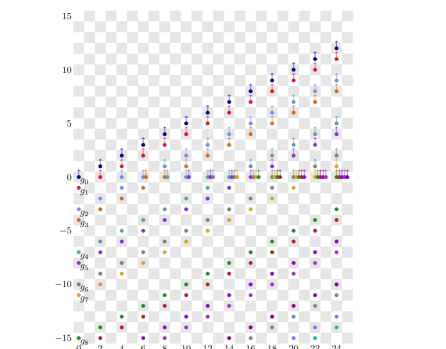
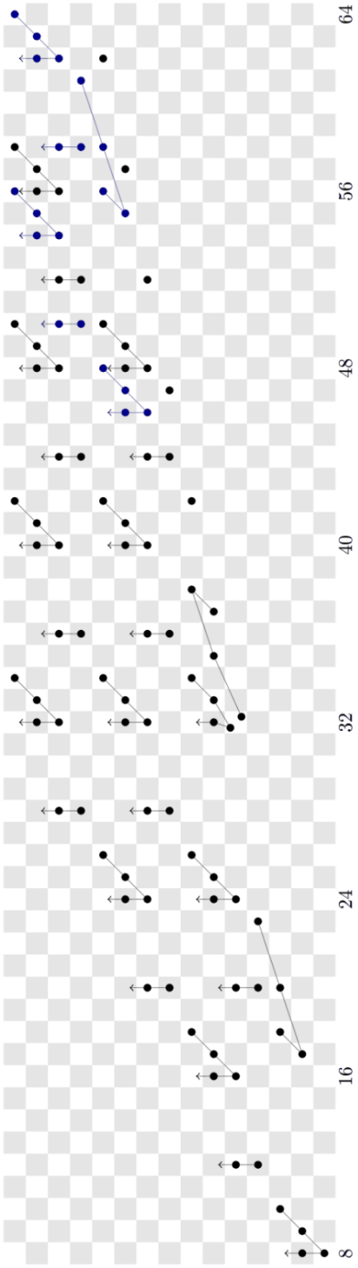
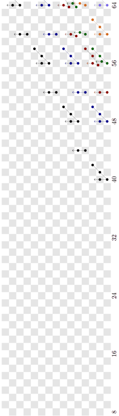
The Adams chart in Figure 3.1 illustrates how the the Mahler basis can be used to identify as a -module inside of . Namely:
-
(1)
Start with the Mahler basis (on the negative -axis).
-
(2)
Draw -towers on each of the .
-
(3)
For each , add a -tower on , starting in non-negative Adams filtration.
Restricted to the first quadrant, this gives the -torsion-free summand of the Adams spectral sequence for .
3.3. The cooperations of and
Adams and Switzer computed along similar lines [Ada74, Sec. II.17]. There is an arithmetic square
which results in a pullback when applying
(One can use the fact that is a -local -Galois extension of to identify the upper right hand corner of the above pullback.) Continuing to let , the bottom map in the above square is given by
We therefore deduce that , with
Again, is similarly determined: since and are -locally equivalent, applying to the arithmetic square yields a pullback square with the same terms on the right hand edge:
We therefore deduce that , with
To produce a basis of this space of functions we use the -Mahler bases developed in [Con00], which we promptly recall. First note that there is an exponential isomorphism
Taking , we have , or in other words, the functions that we are concerned with can be regarded as functions on . They take the form
where is the image of under the isomorphism given by .
To obtain a -Mahler basis as in [Con00] with it is important that . The -Mahler basis is a basis for numerical polynomials with domain restricted to . In the notation of [Con00] we have that
where are coefficients and
Let us set
| (3.5) |
then any is given by
i.e. a basis for is given by the set .
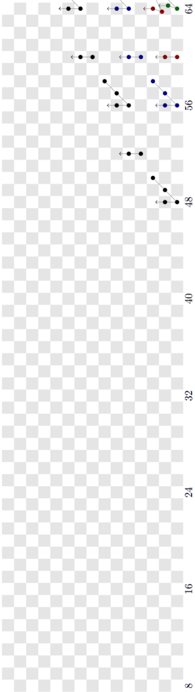
As in the -case, it turns out that the image of in is given by
In order to compute a basis for this we once again need to know the Adams filtration of . One can show that
It follows that we have
Here is a list of the Adams filtration of the first several elements in the -Mahler basis:
| in terms of | ||
|---|---|---|
With this information we can now give the Adams chart (Figure 3.2) of modulo -torsion.
3.4. Calculation of the image of in
We now compute the image (on the level of Adams -terms) of the composite
Since , it suffices to determine the image of the generator
Because the maps
are constructed to be -module maps, everything else is determined by and , i.e. -multiplication. Consider the commutative diagram induced by the maps , , and
On the level of homotopy groups the bottom row of the above diagram takes the form
Since we have
it suffices to find an element such that
Clearly we can take . Note that we have
From the equation
and the fact that the map is one of Hopf algebroids, we deduce that we have
Hence we get that
and thus
Since
by (3.5) we see that we have
so that we can take
We have therefore arrived at the following well-known theorem (see [LM87, Cor. 2.5(a)]).
Theorem 3.6.
The image of the map
is the submodule
Remark 3.7.
For each , this theorem describes a submodule of . These submodules are represented by the different colors in Figure 3.2.
3.5. The embedding into
The final step is to consider the maps of -algebras given by the composite
where is the -th Adams operation. Together, they result in a map of -algebras
Remark 3.8.
The map above has a modular interpretation. Let denote the moduli stack of formal groups, and let
classify with the action of . This map equips with a sheaf of -rings, such that the derived global sections are ; the reader is referred to the appendix of [LN14] for details. The spectrum is the global sections of the pullback
For we may consider the map of stacks
sending to the object . As varies this induces the map .
Proposition 3.9.
The map
is an injection.
Proof.
Consider the diagram
where the bottom horizontal map is the map induced from the inclusion of groups
The vertical maps are injections, since
The bottom horizontal map is an injection since is dense in . The result follows. ∎
We investigated the Brown-Gitler wedge decomposition
and we now end this section by explaining how the map
is compatible with the above decomposition.
Proposition 3.10.
The composites
are equivalences after inverting .
Proof.
This follows from the fact that ∎
Remark 3.11.
In fact, the “matrix” representing the composite
is upper triangular, as we have
| (3.12) |
This is related to a result of Barker and Snaith [BS05] in the following way. They prove that with respect to the decomposition
| (3.13) |
the automorphism
is represented by a matrix conjugate to
Therefore corresponds to a matrix of the form
| (3.14) |
Using the fact that the composite
corresponds to projection on the summand of (3.13), it follows that (3.12) is consistent with the top row of the matrix (3.14).
4. Recollections on topological modular forms
4.1. Generalities
In this subsection, we work integrally. The remainder of this paper is concerned with determining as much information as we can about the cooperations in the homology theory of connective topological modular forms, following our guiding example of . Even more than in the case, an extensive cast of characters will play supporting roles. First of all, we will extensively use the periodic spectrum , which is the analogue of . In particular, we will use the fact that this periodic form of topological modular forms arises as the global sections of the Goerss-Hopkins-Miller sheaf of ring spectra on the moduli stack of smooth elliptic curves . As the associated homotopy sheaves are
there is a descent spectral sequence
Morally, the connective should arise as global sections of an analogous sheaf on the moduli stack of all cubic curves (i.e. allowing nodal and cuspidal singularities); however, this has not been formally carried out. Nevertheless, can be constructed as an -ring spectrum from as a result of the gap in the homotopy of a third, non-connective and non-periodic, version of topological modular forms associated to the compactification of .
Rationally, every smooth elliptic curve is locally isomorphic to a cubic of the form
with the discriminant invertible. Here is a section of the line bundle over the étale map classifying . This translates to the fact that , which in turn implies that The connective version has .
The spectrum of topological modular forms is, of course, not complex orientable, and just like in the case of , we will need the aid of a related complex orientable spectrum. The periodic spectrum admits ring maps to several families of orientable (as well as non-orientable) spectra which come from the theory of elliptic curves. Namely, an elliptic curve is an abelian group scheme, and in particular it has a subgroup scheme of points of order for any positive integer . When is invertible, is locally isomorphic to the constant group . Based on this observation, there are various additional structures that one can assign to an elliptic curve. In this work we will be concerned with two types, the so-called and level structures.
A level structure on an elliptic curve is a specification of a point of (exact) order on , whereas a level structure is a specification of a cyclic subgroup of of order . The corresponding moduli problems are denoted and . Assigning to the pair the pair , where is the subgroup of generated by , determines an étale map of moduli stacks
Moreover, there are two morphisms
which are étale; forgets the level structure whereas quotients by the level structure subgroup. Composing with , we obtain analogous maps from . We can take sections of over the forgetful maps and obtain ring spectra and , ring maps as well as maps of descent spectral sequences
obtained by pulling back. In particular, for any odd integer we have such a situation -locally.
We use the ring map induced by the forgetful to equip with a -module structure. With this convention, the map induced by the quotient map on the moduli stacks does not respect the -module structure. However, one can uniquely extend to
| (4.5) |
Another way to define is as the composition of with the multiplication on .
Finally, we will be interested in the morphism
which is the étale map induced by the multiplication-by- isogeny on an elliptic curve, and the induced map is an Adams operation on .
In Section 7 below, we will make heavy use of the maps and . Their usefulness is due to the relative ease with which their behavior on non-torsion homotopy groups can be computed.
Remark 4.6.
There is a subtlety in defining the maps
which is glossed over in the above discussion. The definition of the map presupposes a canonical identification of the sections of on the étale opens and , and the definition of the map somehow associates a map of spectra to an isogeny of elliptic curves. The real origin of these maps of spectra comes from Lurie’s generalization of the Goerss-Hopkins-Miller Theorem (see [BL10]), which actually presents the -completions of the sheaf as a sheaf on the étale site of the moduli stack of height two -dimensional -divisible groups . The -torsion of an elliptic curve gives a -divisible group . Let
denote the map which forgets level structure and outputs the -divisible group of the underlying elliptic curve (where ). The Serre-Tate theorem implies this map is étale, and is the associated spectrum of sections. Given a cyclic subgroup of order , the isogeny
induces an isomorphism of associated -divisible groups, and hence gives a -cell making the following diagram of stacks homotopy commute:
This induces a map on sections
(see, for instance, [DFHH14, Ch. 5]). The map
is then obtained by constructing the map rationally, and assembling over an arithmetic square. The map
is obtained using the diagram
induced by the isogeny
A different perspective on these maps between -spectra can be found in [Beh09], but that treatment also secretly relies on Lurie’s generalized Goerss-Hopkins-Miller theorem. The reader uncomfortable with relying on unpublished work could also obtain the morphisms and using the obstruction theoretic construction of described in [DFHH14, Ch. 12]: the isogenies induce isomorphisms on formal groups, and the functoriality of the Goerss-Hopkins-Miller theorem gives maps on the localizations of . An explicit map of -algebras corresponding to the respective isogenies gives, via -local obstruction theory, a map of the -localizations of . These assemble via chromatic fracture to give a map on the -completions of for , and these then assemble via the arithmetic square to give the desired maps.
4.2. Details on as
We return to the convention that everything is -local. The significance of in the computation of was that at the prime , is a truncated Brown-Peterson spectrum with a ring map which upon -localization becomes the inclusion of homotopy fixed points . In particular, the image of in homotopy is describable as certain invariant elements. By work of Lawson-Naumann [LN12], we know that there is a -primary form of obtained from topological modular forms; this will be our analogue of in the -cooperations case.
Lawson-Naumann study the (-local) compactification of the moduli stack . Given an elliptic curve (over a -local base), it is locally isomorphic to a Weierstrass curve of the form
A point of order is an inflection point of such a curve; transforming the curve so that the given point is moved to have coordinates puts in the form
| (4.7) |
This is the universal equation of an elliptic curve together with a level structure. The discriminant of this curve is , and . Consequently, . Lawson-Naumann show that the compactification also admits a sheaf of -ring spectra, giving rise to a non-connective and non-periodic spectrum with a gap in its homotopy allowing to take a connective cover which is an -ring spectrum with
This spectrum is complex oriented such that the composite map of graded rings
is an isomorphism [LN12, Theorem 1.1], where the are Hazewinkel generators. Of course, the map classifies the -typicalization of the formal group associated to the curve (4.7), which starts as [Sil86, IV.2], [S+14]:
We used Sage to compute the logarithm of this formal group law, from which we read off the coefficients [Rav86, A2.1.27] in front of as
Now the formula [Rav86, A2.1.1] (in which is understood to be ) allows us to recursively compute the map . For the first few values of , we have that
We can do even more with this orientation of , as
is a morphism of Hopf algebroids. Recall that with and in degree and the right unit is determined by the fact [Rav86, A2.1.27] that
with by convention. On the other hand,
and the right unit sends to . With computer aid from Sage, we can recursively compute the images of each in . As an example, we include here the first three values
| (4.8) | ||||
and rather than urging the reader to analyze the terms, we simply point out the exponential increase of their number. In Section 4.4 we will use the Adams filtration to extract leading terms from these expressions, allowing us to extract meaningful information from these formulas.
Remark 4.9.
Just as we used as a means of porting formulas in to , so we are using to analyze . The reader might wonder why we do not give a complete analysis of . In fact, such an analysis has recently been completed by Culver [Cul17].
4.3. The relationship between and and their connective versions
As we mentioned already, the forgetful map is étale; moreover, . As a consequence, we have a Čech descent spectral sequence
With it, the modular forms can be computed as the equalizer of the diagram
| (4.12) |
in which and are the left and right projection maps. The interpretation is that the -modular forms are precisely the invariant -modular forms.
To be more explicit, note that classifies tuples of elliptic curves with a point of order and an isomorphism of elliptic curves which does not need to preserve the level structures. This data is locally given by
| (4.13) | |||||
such that the following relations hold
| (4.14) | ||||
(Note: For more details on this presentation of , see the beginning of [Sto14, §4]; the relations follow from the general transformation formulas in [Sil86, III.1] by observing that the coefficients must remain zero. See also [Bau08], where is implicitly used to compute the -primary descent spectral sequence for .)
Hence, the diagram (4.12) becomes
(where denotes the relations (4.14)) with being the obvious inclusion and determined by
which is in fact a Hopf algebroid representing . Note that we do not need to localize at but only to invert to obtain this presentation.
As a consequence of this discussion we can explicitly compute that the modular forms are the subring of generated by
| (4.15) |
which in particular determines the map on non-torsion elements.
4.4. Adams filtrations
The maps and respect the Adams filtration, which allows us to determine the Adams filtration on the right hand sides. Recall that
where as usual, . Consequently, , which in turn implies via (4.15) that
| (4.16) |
More precisely, modulo higher Adams filtration (we use to denote equality modulo terms in higher Adams filtration) we have
| (4.17) |
Note that the Adams filtration of each is zero.
4.5. Supersingular elliptic curves and -localizations
At the prime , there is a unique isomorphism class of supersingular elliptic curves; one representative is the Weierstrass curve
over . Recall that a supersingular elliptic curve is one whose formal completion at the identity section is a formal group of height two.111As opposed to an ordinary elliptic curve whose formal completion has height one. These two are the only options. Under the natural map from the moduli stack of elliptic curves to the one of formal groups sending an elliptic curve to its formal completion at the identity section, the supersingular elliptic curves (in fixed characteristic) are sent to the (unique up to isomorphism, by Cartier’s theorem [Rav86, Appendix B]) formal group of height two in that characteristic.
Let denote a formal neighborhood of the supersingular point of , and let denote a formal neighborhood of the characteristic point of height two of . Formal completion yields a map which is used to explicitly describe the -localization of (or equivalently, ) in terms of Morava -theory.
The formal stack has a pro-Galois cover by for the extended Morava stabilizer group . The Goerss-Hopkins-Miller theorem implies in particular that this quotient description of has a derived version, namely the stack , where is a Lubin-Tate spectrum of height two. As we are working with elliptic curves, we take the Lubin-Tate spectrum associated to the formal group over , and .
Let denote the automorphism group of ; it is a finite group of order given as an extension of the binary tetrahedral group with the Galois group of . Then embeds in as a maximal finite subgroup and is a Galois cover of for the group . In particular, taking sections of the structure sheaf over gives the -localization of which is equivalent to . Moreover, we have -local equivalences
The decomposition on the right hand side is interesting though we will not pursue it further in this work. The interested reader is referred to Peter Wear’s explicit calculation of the double cosets in [Wea].
5. The Adams spectral sequence for and -Brown-Gitler modules
Recall that we are concerned with the prime , hence everything is implicitly -localized.
5.1. Rational calculations
Recall that we have
and consider the (collapsing) -inverted ASS
In this section we explain the decomposition imposed on the -term of this spectral sequence from the decomposition on the -term. In particular, given a torsion-free element , this will allow us to determine which -Brown-Gitler module detects it in the -term of the ASS for .
Recall from Section 4 that . In particular, we have
We begin by studying the map between -inverted ASS’s induced by the map
We have
where the ’s have bidegrees:
Recall from Section 4 that , and that
Of course , with corresponding localized Adams -term
where the ’s have bidegrees
Recall also from Section 4 that the formulas for and in terms of and imply that the map of -terms of spectral sequences above is injective, and is given by
| (5.1) |
Corresponding to the isomorphism
there is an isomorphism of localized Adams -terms
Since the decomposition
is a decomposition of -comodules, it is in particular a decomposition of -comodules, and therefore there is a decomposition
| (5.2) |
Proposition 5.3.
Under the decomposition (5.2), we have
Proof.
Statement (2) of the proof of Lemma 3.3 implies that we have
Using the map (2.1), we deduce that we have
Consider the diagram:
| (5.4) |
The map
sends to . Thus the elements
have the same image in . However, using the formulas of Section 4, we deduce that the images of and in
are given by
Since the map
of diagram (5.4) sends to and to zero, we deduce that the image of and in is
It follows that under the map of -localized ASS’s induced by the map
we have
Therefore, by (5.1), we have the equality (in )
and the result follows. ∎
Corresponding to the Künneth isomorphism for , there is an isomorphism
In particular, since the maps
can be identified with the maps
we have the following corollary.
Corollary 5.5.
5.2. Inductive computation of
The exact sequences (2.9),(2.10) provide an inductive method of computing in terms of -computations and .
We give some low dimensional examples. We shall use the shorthand
to denote the existence of a spectral sequence
In the notation above, we shall abbreviate as . We have
| (5.6) |
In practice, these spectral sequences tend to collapse. In fact, in the range computed explicitly in this paper, there are no differentials in these spectral sequences, and the authors have not yet encountered any differentials in these spectral sequences. These spectral sequences collapse with -inverted, for dimensional reasons.
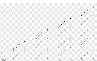
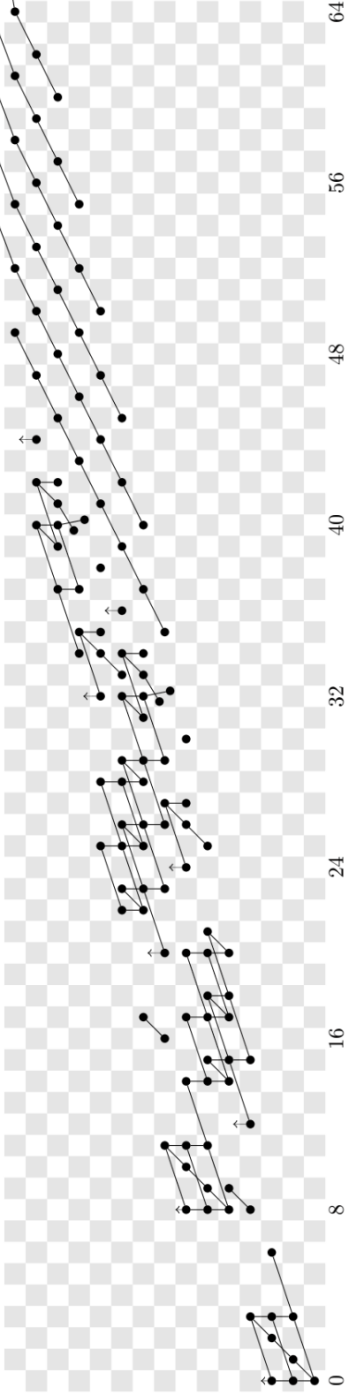
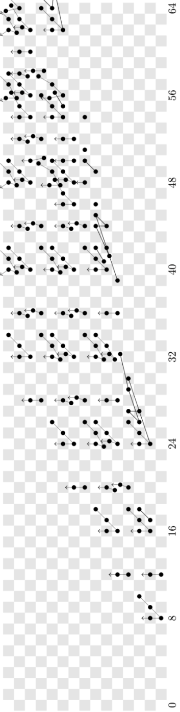
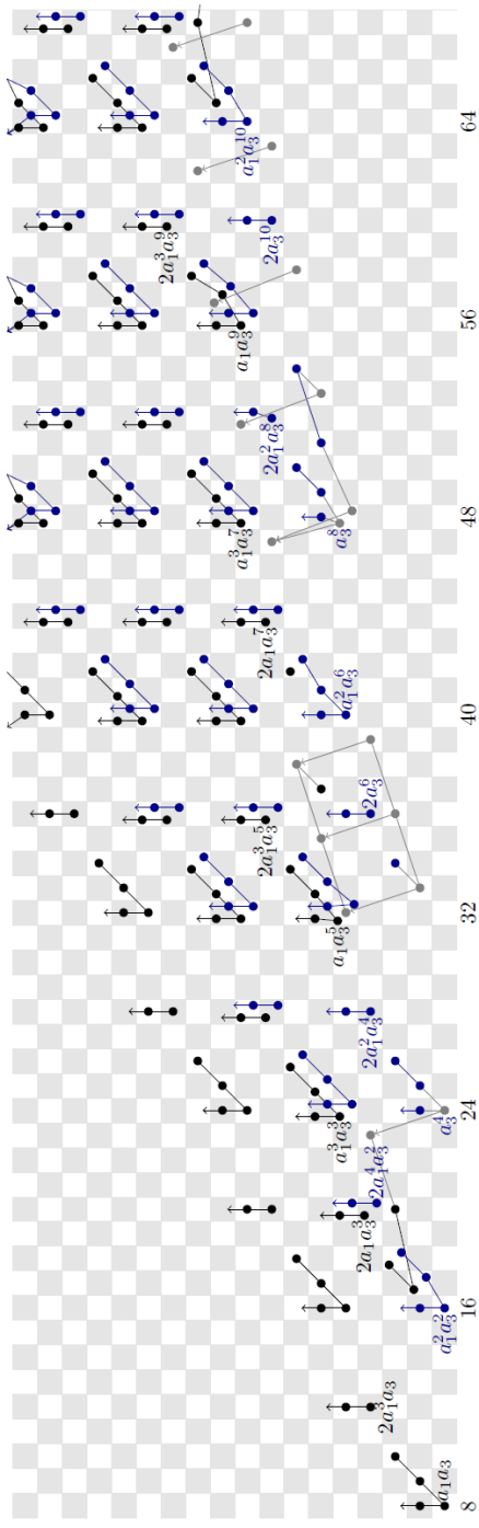
In principle, the exact sequences (2.9) and (2.10) allow one to inductively compute given , where is depicted in Figure 5.1.
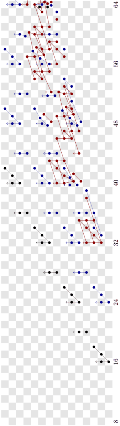
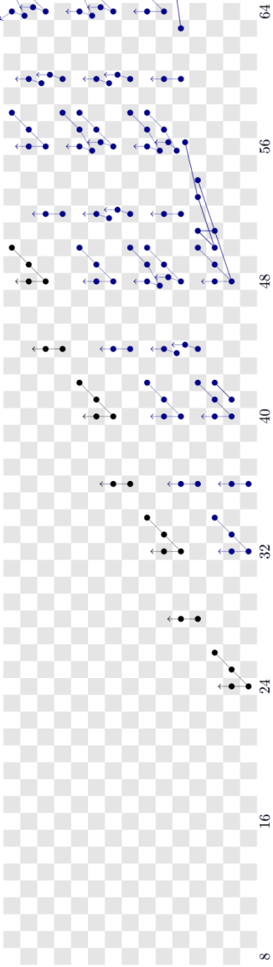
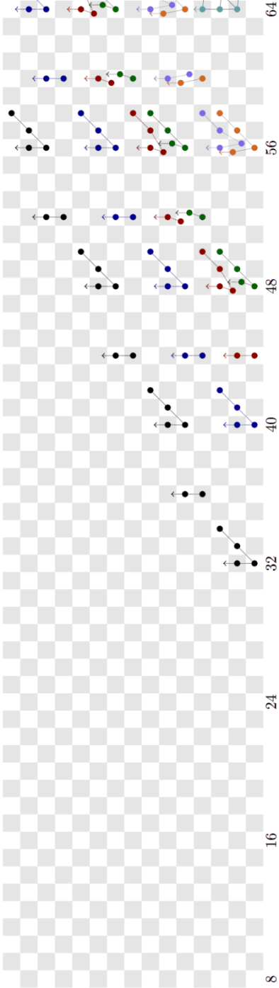
The problem is that, unlike the -case, we do not have a closed form computation of . These computations for appeared in [BHHM08] (the cases of appeared elsewhere). We include in Figures 5.2 through 5.5 the charts for , for , as well as in dimensions . In these figures, the different contributions to coming from the different summands of the -term of the spectral sequences 5.6 are denoted with different colors.
5.3. Rational behavior of the exact sequences
We finish this section with a discussion on how to identify the generators of . On one hand, the inclusion
discussed in Section 5.1 informs us that the -towers of are all generated by
for appropriate (possibly negative) values of depending on and .
The problem is that the terms
| (5.7) | ||||
| (5.8) |
in the short exact sequences (2.9), (2.10) are not free over (however, they are free over ).
We therefore instead identify the generators of corresponding to the generators of (5.7) and (5.8) as modules over , as well as those generators coming (inductively) from
| (5.9) | ||||
| (5.10) |
in the following two lemmas, whose proofs are immediate from the definitions of the maps in (2.9), (2.10).
Lemma 5.11.
Lemma 5.12.
Lemma 5.14.
Consider the summand
generated as a module over by the generators
with . Let () be the generator of the summand (5.13), as a module over corresponding to the generator Then we have
in , where the additional terms not listed above all come from the summand
Proof.
This follows from the definition of the last map in (2.9), together with the fact that with inverted, the cell attaches to the cell with attaching map . ∎
Lemmas 5.11, 5.12, and 5.14 give an inductive method of identifying a collection of generators for , which are compatible with the exact sequences (2.9), (2.10). We tabulate these below for the decompositions arising from the spectral sequences (5.6). For those summands of the form these are generators over , for the other summands these are generators over .
5.4. Identification of the integral lattice
Having constructed useful bases of the summands
it remains to understand the lattices
This can accomplished inductively; the rational generators we identified in the last section are compatible with the exact sequences (2.9), (2.10), and of the terms in these exact sequences are determined by the -computations of Section 3, and knowledge of
Unfortunately the latter requires separate explicit computation for each , and hence does not yield a general answer.
Nevertheless, in this section we will give some lemmas which provide convenient criteria for identifying the so that given a rational generator (as in the previous section) we have
We first must clarify what we actually mean by “rational generator”. The generators identified in the last section originate from the exact sequences (2.9), (5.7). More precisely, they come from the generators of where is given by
| Case 1: | |||
| Case 2: |
In Case 1, a generator of is a generator as a module over , using the isomorphisms
| (5.15) |
The rational generators in this case correspond to the generators
In Case 2, a generator of is a generator as a module over using the isomorphisms
| (5.16) |
The rational generators in this case correspond to the generators
In either case, the maps in both (5.16) and (5.15) arise from surjections of cobar complexes
induced by the surjection
Thus a term representing an element in corresponds (for sufficiently large) to a term . Then we have determined an element of the integral lattice
Lemma 5.17.
Suppose that the -coaction on satisfies
with primitive, as in the following “cell diagram”:
Then
and is represented by
in the cobar complex .
Proof.
Since the cell complex depicted agrees with through dimension , of this comodule agrees with through dimension . In particular, generates an -term in this dimension. To determine the exact representing cocycle, we note that
kills in . ∎
Example 5.18.
Let be a monomial with exponents all divisible by . A typical instance of a set of generators of satisfying the hypotheses of Lemma 5.17 is
The following corollary will be essential to relating the integral generators of Lemma 5.17 to -variable modular forms in Section 6.
Corollary 5.19.
Suppose that satisfies the hypotheses of Lemma 5.17. The image of the corresponding integral generator
in is given by
Proof.
Note the equality
Therefore the image of the integral generator of Lemma 5.17 under the map
is
and this represents . ∎
Similar arguments provide the following slight refinement.
Lemma 5.20.
Suppose that the -coaction on satisfies
with primitive, and that there exists and satisfying
and
as in the following “cell diagram”:
Then
is represented by
in the cobar complex .
Example 5.21.
Let be a monomial with exponents all divisible by . A typical instance of a set of generators of satisfying the hypotheses of Lemma 5.20 is
Corollary 5.22.
Suppose that satisfies the hypotheses of Lemma 5.20. The image of the corresponding integral generator
in is given by
6. The image of in : two variable modular forms
6.1. Review of Baker-Laures work on cooperations
In this brief subsection, we do not work -locally, but integrally.
For , the spectrum is even periodic, with
In particular, its homotopy is torsion-free. As a result, there is an embedding
Consider the multivariate -expansion map
In [Lau99, Thm. 2.10], Laures uses it to determine the image of under the embedding above.
Theorem 6.1 (Laures).
The multivariate -expansion map gives a pullback
Therefore, elements of are given by sums
with
We shall let denote this ring of integral -variable modular forms (meromorphic at the cusps). We shall denote the subring of those integral -variable modular forms which have holomorphic multivariate -expansions by .
Remark 6.2.
Baker [Bak95] showed that in the case of , with inverted, we have
Laures’s methods also apply to this case.
6.2. Representing with -variable modular forms
From now on, everything is again implicitly -local.
We now turn to adapting Laures’s perspective to identify . To do this, we use the descent spectral sequence for
Let denote the Hopf algebroid encoding descent from to , with
(see Section 4) where denotes the relations (4.14). The Bousfield-Kan spectral sequence associated to the cosimplicial resolution
yields a Baker-Lazarev spectral sequence [BL01]
We can use parallel methods to construct a Baker-Lazarev spectral sequence for the extension
Let denote the associated Hopf algebroid encoding descent, with
The Bousfield-Kan spectral sequence associated to the cosimplicial resolution
yields a descent spectral sequence
Lemma 6.3.
The map induced from the edge homomorphism
is an injection.
Proof.
This follows from the fact that the map
induces a map of descent spectral sequences
and the rational spectral sequence is concentrated on the line. ∎
The significance of this homomorphism is that the target is the space of -local two-variable modular forms for .
Lemma 6.4.
The -line of the descent spectral sequence for may be identified with the space of -local two-variable modular forms of level (meromorphic at the cusp):
Proof.
This follows from the composition of pullback squares
The bottom square is a pullback by Theorem 6.1. Note that since is Landweber exact, is torsion-free. Thus an element of is -primitive if and only if its image in is primitive. This shows that the top square is a pullback. ∎
6.3. Representing with -variable modular forms
Recall from Equation 4.16 that the Adams filtration of is 4 and the Adams filtration of is 5. Regarding -variable modular forms as a subring
we shall denote by the subring of 2-variable modular forms with non-negative Adams filtration. The results of the previous section now easily give the following result.
Proposition 6.5.
Proof.
Consider the commutative cube
(The dotted arrow exists because the front face of the cube is a pullback.) The commutativity of the diagram, and the fact that rationally the top face is isomorphic to the bottom face, give an injection
that is a rational isomorphism. Since all of the elements of the source have Adams filtration , this injection factors through the subring
∎
6.4. Detecting -variable modular forms in the ASS
Definition 6.6.
Suppose that we are given a class
and a -variable modular form
We shall say that detects if the image of in detects the image of in in the localized ASS
Remark 6.7.
Suppose as above is a permanent cycle in the unlocalized ASS
and detects . If is the image of under the map
then detects in the sense of Definition 6.6.
Given a class , we wish to find a -variable modular form it detects. To accomplish this, we contemplate the following diagram
| (6.8) |
and the associated “Ext version”:
| (6.9) |
Here, denotes the associated graded with respect to Adams filtration (AF), where, as usual (see Section 4.4), we set
As indicated, in both of the above diagrams, all of the arrows are injections. To determine whether a class detects , it suffices to determine whether the image of in detects the image of in .
The following lemma follows immediately from (4.17).
Lemma 6.10.
The map of Diagram (6.9) is given by
Given a -variable modular form , let denote its image in
and let
denote the element which detects it in the (collapsing) -localized ASS.
Similarly, let denote the images of in (as in Section 4.2), and let denote the elements of which detect these images in the -localized ASS for .
The map of Diagram (6.9) is essentially determined by the following lemma.
Lemma 6.11.
Proof.
The elements are easily checked to be primitive with respect to the -coaction. The second part follows from the fact that in the diagram
is mapped to by the top horizontal map. ∎
Remark 6.12.
We assemble these observations to give the following convenient criterion for determining when a particular element detects a -variable modular form .
Proposition 6.13.
Suppose that we are given an element whose image in
is given by
with . The element detects a -variable modular form
if and only if
6.5. Low dimensional computations of -variable modular forms
Below is a table of generators of , as a module over , through dimension 64, with -variable modular forms they detect. The columns of this table are:
- dim:
-
dimension of the generator,
- :
-
indicates generator lies in the summand (see the charts in Section 5),
- AF:
-
the Adams filtration of the generator,
- cell:
-
the name of the image of the generator in , in the sense of Section 5.3,
- form:
-
a two-variable modular form which is detected by the generator in the -localized ASS (where are defined below).
The table below also gives a basis of as a -module: in dimension , a form in the last column, with and a monomial in not divisible by 2, corresponds to a generator of .222There is one exception: there is a -variable modular form which agrees with modulo terms of higher Adams filtration, but which is -divisible. See Example 7.12.
The -variable modular forms in the above table are the generators of as an -algebra in this range, and are defined as follows.
We shall now indicate the methods used to generate Table 1, and make some remarks about its contents.
The short exact sequences (2.9),(2.10) were used in Section 5.2 to give an inductive scheme for computing , and the charts in that section display the computation through dimension . In Section 5.3, these short exact sequences are used to give an inductive scheme for identifying the generators of , and appropriate multiples of these generators generate the image of in these localized Ext groups. These generators are listed in the fourth column of Table 1.
The two variable modular forms in the last column of Table 1 are detected by the generators in the fourth column, in the sense of the previous section. In each instance, if necessary, we use Corollary 5.19 or 5.22 to find the image of the generator in and then apply Proposition 6.13.
The 2-variable modular forms were generated by the following inductive method. Let be a basis of
as an -module. We wish to produce a basis
such that for appropriate , the detects . Suppose inductively that we have found such -variable modular forms for all with Adams filtration (AF) greater than , and let be a basis element with . We wish to produce a -variable modular form such that detects , and so that
This will be accomplished by writing a finite sequence of approximations
with
and
We will then take and .
- Step 1:
-
Find an element
so that
Such an can be produced in one of two ways:
- Technique (a):
- Technique (b):
-
If , where inductively you already have -variable modular forms which detect, you may also take to be
- Step 2:
-
Write the -expansion of as
where is the -expansion of 2-integral 2-variable modular form.
- Step 3:
-
Write as a linear combination of the -expansions of the -variable modular forms of Adams filtration greater than already produced mod :
- Step 4:
-
Set
Then
and
where is a -integral -variable modular form.
- Step 5:
-
Repeat steps 3 and 4 to inductively produce .
We explain all of this by working it through some low degrees:
- :
-
The corresponding generator of is . Using “Technique (a)”, we compute the image of in to be
Using Lemma 6.10, we take
We find that has an integral -expansion, and therefore take
- :
- :
-
The corresponding generator of is . Since detects , we can simply use “Technique (b)” to get
The process terminates here, as is -integral since is.
- :
-
The corresponding generator of is . Again we use “Technique (b)”. Since detects and detects , detects .
- :
-
The corresponding generator of is . Since detects , we use “Technique (b)” to begin with
This -variable modular form is not -integral, but the form
is integral (“Step 2”). Moving on to “Step 3”, we find
We define
It turns out (“Step 4”)
Therefore we define
In fact
so we set
and
7. Approximating by level structures
Recall from §4 the maps
and
Here is induced by the forgetful and quotient maps , while where is the “Adams operation” associated to the multiplication by isogeny on . For reasons which will become clear in the next section, we are interested in the composite map given as
where
We will abuse notation and refer to the composite
(for ) as as well; these are the factors of .
In order to study we consider the square
Here the left-hand vertical map is the composite
and is the ring of level -modular forms. The bottom horizontal map is also induced by and ; if we consider a -variable modular form as a polynomial , then .
We are especially interested in the cases . Recall from [MR09] (or [BO16, §3.3]) that has a convenient presentation as a subalgebra of . More precisely, with , and is the subring
Using the formulas from loc. cit., we may compute
There are similar formulas for the case which we recall from [BO16, §3.4]. Here the ring of -modular forms takes the form
where and . (These are the algebraic, rather than topological, degrees.) The discriminant takes the form
and we have
7.1. Faithfullness of
In this section we will prove the following theorem.
Theorem 7.1.
The map on homotopy
induced by the map defined in the last section is injective.
Theorem 7.1 will be proven in two steps. Consider the following diagram
| (7.2) |
where the vertical maps are the localization maps. We will first argue that the left vertical map in (7.2) is injective, and we will observe that the same argument shows the right hand vertical map is injective. Secondly, we will show that the bottom horizontal map of (7.2) is injective. Theorem 7.1 then follows from the commutativity of (7.2) and these injectivity results.
Lemma 7.3.
The localization map
is injective.
Proof.
Since is -local, we have
where above run over a suitable cofinal range of . In order to conclude that there is an isomorphism
and for the map
to be injective we must show that no element of is infinitely divisible by elements of the ideal . Consider the Adams-Novikov spectral sequence for . This spectral sequences converges since is -local [HS99, Thm. 5.3]. The -term of this spectral sequence is easily seen to not be infinitely divisible by elements of the ideal . Therefore, any infinite divisibility in would have to occur through infinitely many hidden extensions. This would result in elements in negative Adams-Novikov filtration, which is impossible. ∎
The same argument shows that the various maps
are injections. The only remaining step to proving Theorem 7.1 is to show the bottom arrow of Diagram (7.2) is an injection. This is the heart of the matter.
Lemma 7.4.
The map
is an injection.
In order to prove this lemma, we will need the following technical observation.
Lemma 7.5.
Suppose that is a profinite group, is a finite subgroup of , and is an open subgroup of containing . Then there is a finite set of open subgroups which contain , and a corresponding finite set of elements in such that
-
(1)
forms an open cover of , and
-
(2)
Proof.
We have
(where we use to denote “open subgroup”). Therefore, for each , we have
Therefore, for each with , there must be a subgroup so that . Define
(If the set of all such is empty, define .) Since is finite, this is a finite intersection, hence is open. Note that has the property that and
Consider the cover where ranges over the elements of . Since is compact, there is a finite subcover . We may therefore take . ∎
Proof of Lemma 7.4.
Let denote the second Morava stabilizer group, and let denote the version of Morava -theory associated to a height formal group over . The spectrum admits an action by the group where is the Galois group of over , and we have
where is the group of automorphisms of the (unique) supersingular elliptic curve over . In [GHMR05], it is shown that this homotopy fixed point description of gives rise to the following description of
There is a subtlety being hidden with the above notation: the Galois group is acting on the continuous mapping spectrum with the conjugation action, where it acts on the source through the left action on
For coprime to , let denote the groupoid whose objects are pairs where is a supersingular elliptic curve over and is a cyclic subgroup of order , and whose morphisms are isomorphisms of elliptic curves which preserve the subgroup. Then we have
For a prime , let denote the groupoid whose objects are quasi-isogenies
with supersingular curves over , and whose morphisms from to are pairs of isomorphisms making the following square commute
It is easy to see that there is an equivalence of groupoids
given by sending a pair to the quasi-isogeny given by the composite
However, since there is a unique supersingular elliptic curve over , the category admits the following alternative description (we actually only need that is unique up to -power isogeny). Let denote the group of quasi-isogenies whose order is a power of . There is an inclusion
given by associating to a quasi-isogeny the associated automorphism of the formal group . Then there is a bijection between the isomorphism classes of objects of and the double cosets
Moreover, given an element , the corresponding automorphisms of the associated object in is the group
Putting this all together, we have
and under the equivalences described above, the map
can be identified with the map
| (7.6) |
induced by the map
| (7.7) |
In [BL06] it is shown that the image of the above map is dense. Intuitively, one would like to say that this density implies that a continuous function on is determined by its restrictions to and , and this should imply that the map (7.6) is injective on homotopy. The difficulty lies in making this argument precise.
Before we make the argument precise (which is rather technical) we pause to give the reader an idea of the intuition behind the argument. An element in
is something like a section of a sheaf over whose stalk over is
One would like to say a section of this sheaf is trivial if its values on the stalks are trivial. However, the actual space of continuous maps is a (-local) colimit of maps
so an element of the homotopy of the continuous mapping space is actually represented by a kind of locally constant section with constant value over lying in the group
The difficulty is that there are only maps
and these maps are not necessarily injections. The point of Lemma 7.5 is that the open cover of given by the double cosets admits a finite refinement, over which the “constant sections” have values in one of the stalks, and hence the vanishing of a value at a stalk implies the vanishing of the constant section.
We now make this argument completely precise. We have
and
for suitable pairs . Consider the natural maps
Lemma 7.4 will be proven if we can show that if we are given an open subgroup and a sequence in the product
such that
for , then there is another subgroup such that the associated sequence
is zero, where is the restriction to of .
Suppose that is such a sequence in the kernel of and . Take a cover of as in Lemma 7.5, and let . Regarding and as subgroups of , the density of the image of the map (7.7) implies that the map
is surjective. We therefore may assume without loss of generality that the elements are either in or . We need to show that the associated sequence is zero. Take a representative of a double coset . Then for some . Note that we therefore have
Consider the associated composite of restriction maps
The element is the image of under the above composite. However, since is in the kernel of and , it follows that the image of is zero in
We therefore deduce that is zero, as desired. ∎
7.2. Computation of and in low degrees
Using the formulas for and for and in the beginning of this section, we now compute the effect of the maps and on a piece of . Using the notation of (5.6), we have decompositions:
As indicated by the underbraces above, we shall refer to the first piece of as , and the second piece as , and the first piece of as .
We define a -lattice of to be a -submodule which is finitely generated as a -module, and has the property that
Note that the first condition forces to be concentrated in for some .
We will show that a portion of detected by
in the ASS maps isomorphically onto a -lattice of , recovering an observation of Davis, Mahowald, and Rezk [MR09], [DM10]. Similarly, we will show that a portion of detected by
in the ASS maps isomorphically onto a -lattice of . This is a new phenomenon.
Actually, Davis, Mahowald, and Rezk proved something stronger in [MR09], [DM10]: they showed (-locally) that there is actually a -module
which maps to as a connective cover, in the sense that on homotopy groups it gives the aforementioned -lattice. In the last section of this paper we will reprove and strengthen their result, and show that there is also a (-local) -module
(where is a -module whose cohomology is isomorphic to the cohomology of as an -module) which maps to as a connective cover, topologically realizing the corresponding -lattice of .
It will turn out that to verify these computational claims, it will suffice to compute the maps
rationally. The behavior of the torsion classes will then be forced.
The case of .
Observe that we have
Recall that
(regarded as a subring of ). For a modular form , we will write
where we have
-
(1)
, and
-
(2)
We shall refer to as the leading term of .
The forgetful map
is computed on the level of leading terms by
Using the formulas for and given in the beginning of this section, we have
| (7.8) |
It follows that on the level of leading terms, the -submodule of given by
maps under to the -lattice given by the ideal
expressed as
The case of .
Observe that we have
Recall that
For a modular form , we will write
where and
-
(1)
, and
-
(2)
We shall refer to as the leading term of .
The forgetful map
is computed on the level of leading terms by
Unlike the case of , the -submodule of -variable modular forms generated by the forms listed above in
does not map nicely into . Rather, we choose different generators as listed below. These generators were chosen inductively (first by increasing degree, and second, by decreasing Adams filtration) by using a row echelon algorithm based on leading terms (see Examples 7.11 and 7.12). In every case, a generator named agrees with modulo terms of higher Adams filtration:
| (7.9) |
The following forms, while not detected by , will be needed:
We now define:
Again, the following forms are not detected by , but will be needed:
We then define:
Using the formulas for and given in the beginning of this section, we have
| (7.10) |
Example 7.11.
We explain how the above generators were produced by working through the example of .
- Step 1:
-
Add terms to of higher Adams filtration to ensure that . For example, we compute
According to (7.8), we have . Since has higher Adams filtration, we can add it to without changing the element detecting it in the ASS, to cancel the leading term of . We compute
Again, using (7.8), we see that (of higher Adams filtration) also has this leading term, so we now compute:
We see that also has this leading term, and
- Step 2:
-
Add terms to to ensure that the leading term of is distinct from those generated by elements in lower degree, or higher Adams filtration. In this case, we compute
By induction we know the leading term of on generators in lower degree and higher Adams filtration, and in particular (7.10) tells us that this leading term is distinct from leading terms generated from elements of lower degree. We therefore define
Example 7.12.
We now explain a subtlety which may arise by working through the example of .
- Step 1:
-
We would normally add terms to of higher Adams filtration to ensure that . Of course, because we already know that , we have
- Step 2:
-
We now add terms to to ensure that the leading term of is distinct from those generated by elements in lower degree. In this case, we compute
By induction we know the leading term of on generators in lower degree and higher Adams filtration, but now (7.10) tells us that
Since has higher Adams filtration, we add it to and compute
We inductively know that , and we compute
We inductively know that , and we compute
In other words, the expression above is congruent to mod , and therefore the leading term is divisible by ! However, this leading term is distinct from leading terms generated from elements of lower degree, so we define
and record the leading term of as . (In fact, the 2-variable modular form is -divisible, and this is why some of the equations in (7.9) involve the term .)
7.3. Using level structures to detect differentials and hidden extensions in the ASS
In the previous section we observed that maps a -submodule of detected in the ASS by
to a -lattice , and maps a -submodule of detected in the ASS
to a -lattice .
We now observe that using the known structure of and , we can deduce differentials in the portion of the ASS detected by
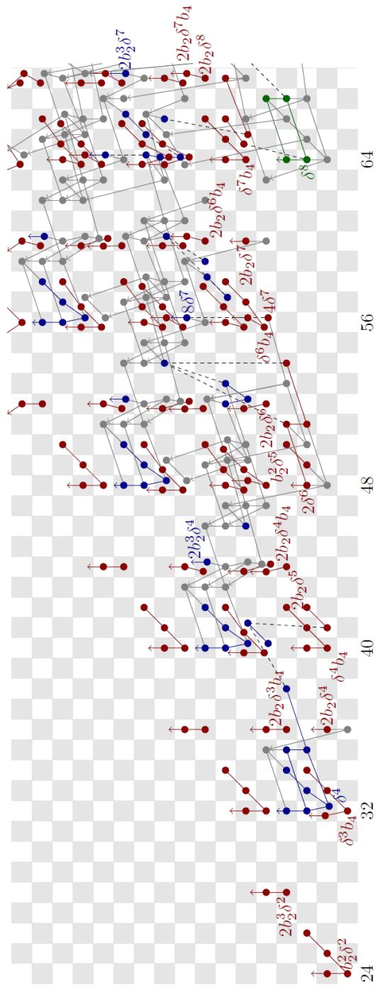
We begin with . Figure 7.1 displays this portion of the -term of the ASS for , with differentials and hidden extensions. The -generators in the chart are also labeled with -modular forms. These are the leading terms of the -modular forms that they map to under the map (see (7.8)). The Adams differentials and hidden extensions are all deduced from the behavior of on these torsion-free classes, as we will now explain. We will also describe how the -torsion in this portion of the ASS detects homotopy classes which map isomorphically under onto torsion in . We freely make reference to the descent spectral sequence
as computed in [MR09].
- Stem 17:
-
We have
Mahowald and Rezk [MR09] define a class in such that
There is a class in such that
The class is a permanent cycle, and detects an element . We deduce
- Stem 24:
-
The modular form is not a permanent cycle in the descent spectral sequence for . It follows that the corresponding element of must support an ASS differential. There is only one possible target for this differential.
- Stem 33:
-
There is a class satisfying
There are no possible non-trivial differentials supported by . Dividing both sides of
by , we deduce that there is an element detected by satisfying
Since is not -divisible, we deduce that must support an Adams differential, and there is only one possible target for such a differential. Since
it follows that the element detects , which maps to under . We then deduce that
- Stem 48:
-
Let denote the unique non-trivial class with , so that is the unique class in that bidegree which supports non-trivial and -multiplication. Note that there is only one potential target for an Adams differential supported by or . Since supports non-trivial and multiplication, it follows that must be a permanent cycle in the ASS, detecting an element satisfying
Since is not -divisible, we conclude that cannot be a permanent cycle. We deduce using -multiplication (i.e. application of ) that
for , and that
We now proceed to analyze . Figure 7.2 displays this portion of the -term of the ASS for , with differentials and hidden extensions. The -generators in the chart are also labeled with -modular forms. These are the leading terms of the -modular forms that they map to under (see (7.10)). As in the case of , the Adams differentials and hidden extensions are all deduced from the behavior of on these torsion-free classes. We will also describe how the -torsion in this portion of the ASS detects homotopy classes which map isomorphically under onto torsion in . We freely make reference to the descent spectral sequence
as computed in [BO16], for instance. Most of the differentials and extensions follow from the fact that the element which generates
must be a permanent cycle in the ASS, and that the ASS for is a spectral sequence of modules over the ASS for
Below we give some brief explanation for the main differentials and hidden extensions which do not follow from this.
- Stem 36:
-
We have
Since is not a permanent cycle in the descent spectral sequence for , we deduce that must support a differential. There is only one possibility (taking into account the differential coming from ),
This is especially convenient, in light of the fact that .
- Stem 41:
-
The hidden extension follows from dividing
by .
- Stem 54:
-
The three hidden extensions to the element all follow from the fact that is non-trivial, and that
- Stem 56:
-
The hidden extension follows from the Toda bracket manipulation
- Stem 64:
-
The differential on follows from the fact that is not -divisible. The hidden extensions follow from the fact that and .
- Stem 65:
-
The hidden -extension follows from the fact that is -divisible, and .
7.4. Connective covers of and in the -resolution
In this section we will topologically realize the summands
of , which we showed detect -submodules that map to -lattices of and under the maps and , respectively. From now on, everything is implicitly -local.
For the purposes of context, we shall say that a spectrum
over is a -Brown-Gitler spectrum if the induced map
maps isomorphically onto one of the -subcomodules defined in Section 5.
Not much is known about the existence of -Brown-Gitler spectra, but the most optimistic hope would be that the spectrum admits a filtration by -Brown-Gitler spectra . The case of is trivial (define ) and the case of is almost as easy: a spectrum can be defined to be the -skeleton:
In light of the short exact sequences
one would anticipate that such -Brown-Gitler spectra would be built from -Brown-Gitler spectra, so that
Davis, Mahowald, and Rezk [MR09], [DM10] nearly construct a spectrum ; they show that there is a subspectrum
(where is the cofiber of the unit ) realizing the subcomodule
We will not pursue the existence of -Brown-Gitler spectra here, but instead will consider the easier problem of constructing the beginning of a potential filtration of by -modules, which we denote even though we do not require the existence of the individual spectra . We would have
such that the map
maps onto the sub-comodule
Note that in the case of , we may take
Since this is the inclusion of a summand, with cofiber denoted , it suffices to instead look for a filtration
of -modules. Our previous discussion indicates that the cases of is easy, and now the work of Davis-Mahowald-Rezk fully handles the case of . In this section we will address the case of , and a “piece” of the case of . We state a proposition and two theorems before moving onto their proofs.
Proposition 7.13.
-
(1)
There is a -module
which realizes the submodule
where is a -module with
(but which may not be equivalent to as a -module).
-
(2)
There is a map of -modules
and an extension
-
(3)
There is a modified Adams spectral sequence
and the map induces a map from this modified ASS to the ASS for such that the induced map on -terms is the inclusion of the summand
In [MR09],[DM10], Davis, Mahowald, and Rezk construct a map
such that cofiber has an ASS with -term
and there is an equivalence
What they do not address is how this connective cover is related to and the map to .
Theorem 7.14.
We also will provide the following analogous connective cover of .
Theorem 7.16.
The remainder of this section will be devoted to proving Proposition 7.13, Theorem 7.14, and Theorem 7.16. The proofs of all of these will be accomplished by taking fibers and cofibers of a series of maps, using brute force calculation of the ASS. These brute force calculations boil down to having low degree computations of the groups for various small values of and . The computations were performed using R. Bruner’s -software [Bru93]. The software requires module definition input that completely describes the -module structure of the modules . The first author was fortunate to have an undergraduate research assistant, Brandon Tran, generate module files using Sage.
Proof of Proposition 7.13.
Endow with a minimal -cell structure corresponding to an -basis of . Let denote the -skeleton of this -cell module, so we have
| (7.18) |
We first wish to form a -module with
| (7.19) |
by taking the fiber of a suitable map of -modules
We use the ASS
The decomposition (7.18) induces a corresponding decomposition of groups. The only non-zero contributions near come from , , and ; the corresponding charts are depicted below.
![[Uncaptioned image]](/html/1501.01050/assets/x13.png)
The generator would detect the desired map . We just need to show that this generator is a permanent cycle in the ASS. As the charts indicate, the only potential target is the non-trivial class
We shall call the potential obstruction for ; if then we will say that is obstructed by . The key observation is that in the vicinity of , the groups are depicted below.
![[Uncaptioned image]](/html/1501.01050/assets/x14.png)
Under the map of ASS’s
the potential obstruction maps to the nonzero class
Therefore if is obstructed by , then is the obstruction to the existence of a corresponding map of -modules
However, Bailey showed in [Bai10] that there is a splitting of -modules
In particular, the map is realized by restricting the splitting map
to -skeleta (in the sense of -cell spectra). Therefore, is unobstructed, and we deduce that cannot be obstructed.
The -module may then be defined to to be the fiber of a map
which on homology is the projection on the summand
Again, we use the ASS
The -term is computed using the decomposition (7.19). The only non-zero contributions come from the following summands:
![[Uncaptioned image]](/html/1501.01050/assets/x15.png)
We discover that the only potential obstruction to the existence of is the non-trivial class
Unfortunately we cannot simply imitate the argument in the previous paragraph, because is in the kernel of the homomorphism
Nevertheless, a more roundabout approach will eliminate this potential obstruction. We first observe that there is a map of -modules
(with denoting the quotient ), which on homology is the canonical composite
The existence of is verified by the ASS
The -term is computed using the decomposition (7.19). The only non-zero contributions in the vicinity of come from the following summands:
![[Uncaptioned image]](/html/1501.01050/assets/x16.png)
We see that there are no potential obstructions for the existence of . Let denote the fiber of , so that we have
| (7.20) |
We instead contemplate the potential obstructions to the existence of a map of -modules
which on homology induces the projection
The -term of the ASS
is computed using the decomposition (7.20), and in particular the contribution coming from the summand gives the following classes in the vicinity of :
![[Uncaptioned image]](/html/1501.01050/assets/x17.png)
We see that there are many potential obstructions to the existence of in
The potential obstructions for the related map
of -modules in the ASS
may be analyzed, and the contribution coming from the summand gives the following classes in the vicinity of :
![[Uncaptioned image]](/html/1501.01050/assets/x18.png)
We see that there is one potential obstruction to the existence of in
We analyze these potential obstructions through the following zig-zag of ASS’s:
In the above diagram the potential obstruction to the existence of maps under to a non-trivial class, so that if obstructs , then obstructs the composite
The key fact to check using Bruner’s -software is that in bidegree , the maps and are both surjective, with the same kernel. It follows that if is obstructed by , then the map
is obstructed. We may now avail ourselves of the Bailey splitting of : the map is unobstructed, because it is realized by the projection
We conclude that cannot obstruct the existence of . We may therefore define to be the fiber of the map .
We now need to show that the -module is built as
In order to establish this decomposition, our first task is to construct a map of -modules
by analyzing the ASS
The only contributions in the vicinity of come from the summands and of :
![[Uncaptioned image]](/html/1501.01050/assets/x19.png)
As we see from the charts above there is a potential obstruction to the existence of in
The Bailey splitting does not eliminate this potential obstruction, as
However, by Toda’s Realization Theorem [Tod71], [BE16, Sec.3], this potential obstruction also corresponds to the existence of a different “form” of the -module , with the same homology. Since for , both forms are realized. It follows that if is obstructed with the standard form, then it is unobstructed for the other form. Let be the unobstructed form, so that there exists a map
The fiber of is , where
is the spectrum constructed by Davis, Mahowald, and Rezk. We note that there is a fiber sequence
since a quick check of reveals there are no exotic “forms” of for , and is the -skeleton of the -cell complex .
We now must produce the map of -modules
This just corresponds to an element . In the ASS
there is a class
(see Figure 5.4). Moreover, according to Figures 5.3 and 5.4, there are no possible targets of an Adams differential supported by this class. Therefore, corresponds to a permanent cycle: take to be the element in homotopy detected by it. The factorization
exists because the element , when regarded as an element of the ASS
is the target of a differential
(see Figure 7.2).
The modified ASS
is constructed by taking the modified Adams resolution
where the map is the composite
is a section of the inclusion
is the fiber of , and is the fiber of the map
The map from this modified ASS to the ASS for arises from the existence of a commutative diagram
(This diagram commutes since the class killing in the ASS for has Adams filtration .) ∎
Proof of Theorem 7.14.
Define a -variable modular form
so that and . (This form was produced by executing an integral variant of the “row-reduction” method outlined in Step 1 of Example 7.11.) Then we may take the attaching map
to be the map of -modules corresponding to the homotopy class
We define
Since , there is a factorization
The rest of the theorem is fairly straightforward given this, and our analysis of in the previous section. ∎
Proof of Theorem 7.16.
An analysis of the Adam -terms in low dimensions reveals that the only non-trivial attaching map of -modules
must factor as
| (7.21) |
where is the unique non-trivial class in that degree. The existence of differentials in Figure 7.2 from -classes to -classes implies that in , must be attached non-trivially to , and we therefore have
When applied to the factorization (7.21), Verdier’s Axiom implies that there is a fiber sequence
Now, an easy check with the ASS reveals that the composite
is null, from which it follows that there is a lift
Define
Verdier’s axiom, applied to the factorization above, gives a fiber sequence
Given our analysis of , the rest of the statements of the theorem are now fairly straightforward. ∎
References
- [Ada74] J. F. Adams, Stable homotopy and generalised homology, University of Chicago Press, Chicago, Ill., 1974, Chicago Lectures in Mathematics. MR 0402720 (53 #6534)
- [Bai10] Scott M. Bailey, On the spectrum , J. Pure Appl. Algebra 214 (2010), no. 4, 392–401. MR 2558747 (2010i:55011)
- [Bak95] Andrew Baker, Operations and cooperations in elliptic cohomology. I. Generalized modular forms and the cooperation algebra, New York J. Math. 1 (1994/95), 39–74, electronic. MR 1307488 (96b:55004)
- [Bau08] Tilman Bauer, Computation of the homotopy of the spectrum tmf, Groups, homotopy and configuration spaces, Geom. Topol. Monogr., vol. 13, Geom. Topol. Publ., Coventry, 2008, pp. 11–40. MR 2508200
- [BE16] Prasit Bhattacharya and Phillip Egger, A class of -local finite spectra which admit a -self map, arXiv:1608.06250, 2016.
- [Beh09] Mark Behrens, Congruences between modular forms given by the divided family in homotopy theory, Geom. Topol. 13 (2009), no. 1, 319–357. MR 2469520
- [BG73] Edgar H. Brown, Jr. and Samuel Gitler, A spectrum whose cohomology is a certain cyclic module over the Steenrod algebra, Topology 12 (1973), 283–295.
- [BHHM08] M. Behrens, M. Hill, M. J. Hopkins, and M. Mahowald, On the existence of a -self map on at the prime 2, Homology, Homotopy Appl. 10 (2008), no. 3, 45–84. MR 2475617 (2009j:55015)
- [BL01] Andrew Baker and Andrej Lazarev, On the Adams spectral sequence for -modules, Algebr. Geom. Topol. 1 (2001), 173–199. MR 1823498
- [BL06] Mark Behrens and Tyler Lawson, Isogenies of elliptic curves and the Morava stabilizer group, J. Pure Appl. Algebra 207 (2006), no. 1, 37–49.
- [BL10] by same author, Topological automorphic forms, Mem. Amer. Math. Soc. 204 (2010), no. 958, xxiv+141. MR 2640996
- [BO16] Mark Behrens and Kyle Ormsby, On the homotopy of and at the prime 2, Algebr. Geom. Topol. 16 (2016), no. 5, 2459–2534. MR 3572338
- [BR08] Andrew Baker and Birgit Richter, On the cooperation algebra of the connective Adams summand, Tbil. Math. J. 1 (2008), 33–70. MR 2434436 (2009d:55012)
- [Bru93] Robert R. Bruner, in the nineties, Algebraic topology (Oaxtepec, 1991), Contemp. Math., vol. 146, Amer. Math. Soc., Providence, RI, 1993, pp. 71–90. MR 1224908 (94a:55011)
- [BS05] Jonathan Barker and Victor Snaith, as an upper triangular matrix, -Theory 36 (2005), no. 1-2, 91–114 (2006). MR 2274160
- [CCW01] Francis Clarke, M. D. Crossley, and Sarah Whitehouse, Bases for cooperations in -theory, -Theory 23 (2001), no. 3, 237–250. MR 1857208 (2002h:55019)
- [CCW05] Francis Clarke, Martin Crossley, and Sarah Whitehouse, Algebras of operations in -theory, Topology 44 (2005), no. 1, 151–174. MR 2104006 (2006b:55015)
- [CJ92] Francis Clarke and Keith Johnson, Cooperations in elliptic homology, Adams Memorial Symposium on Algebraic Topology, 2 (Manchester, 1990), London Math. Soc. Lecture Note Ser., vol. 176, Cambridge Univ. Press, Cambridge, 1992, pp. 131–143. MR 1232203 (94i:55010)
- [Coh81] Ralph L. Cohen, Odd primary infinite families in stable homotopy theory, Mem. Amer. Math. Soc. 30 (1981), no. 242, viii+92.
- [Con00] Keith Conrad, A -analogue of Mahler expansions. I, Adv. Math. 153 (2000), no. 2, 185–230. MR 1770929 (2001i:11140)
- [Cul17] Dominic Culver, On cooperations, arXiv:1708.03001, 2017.
- [DFHH14] Christopher L. Douglas, John Francis, André G. Henriques, and Michael A. Hill (eds.), Topological modular forms, Mathematical Surveys and Monographs, vol. 201, American Mathematical Society, Providence, RI, 2014. MR 3223024
- [DM10] Donald M. Davis and Mark Mahowald, Connective versions of , Int. J. Mod. Math. 5 (2010), no. 3, 223–252.
- [GHMR05] P. Goerss, H.-W. Henn, M. Mahowald, and C. Rezk, A resolution of the -local sphere at the prime 3, Ann. of Math. (2) 162 (2005), no. 2, 777–822.
- [GJM86] Paul G. Goerss, John D. S. Jones, and Mark E. Mahowald, Some generalized Brown-Gitler spectra, Trans. Amer. Math. Soc. 294 (1986), no. 1, 113–132. MR 819938
- [HS99] Mark Hovey and Hal Sadofsky, Invertible spectra in the -local stable homotopy category, J. London Math. Soc. (2) 60 (1999), no. 1, 284–302. MR 1722151 (2000h:55017)
- [Lau99] Gerd Laures, The topological -expansion principle, Topology 38 (1999), no. 2, 387–425.
- [LM87] Wolfgang Lellmann and Mark Mahowald, The -Adams spectral sequence, Trans. Amer. Math. Soc. 300 (1987), no. 2, 593–623.
- [LN12] Tyler Lawson and Niko Naumann, Commutativity conditions for truncated Brown-Peterson spectra of height 2, J. Topol. 5 (2012), no. 1, 137–168. MR 2897051
- [LN14] by same author, Strictly commutative realizations of diagrams over the Steenrod algebra and topological modular forms at the prime 2, Int. Math. Res. Not. IMRN (2014), no. 10, 2773–2813. MR 3214285
- [Mah77] Mark Mahowald, A new infinite family in , Topology 16 (1977), no. 3, 249–256.
- [Mah81] by same author, -resolutions, Pacific J. Math. 92 (1981), no. 2, 365–383. MR 618072 (82m:55017)
- [Mil75] R. James Milgram, The Steenrod algebra and its dual for connective -theory, Conference on homotopy theory (Evanston, Ill., 1974), Notas Mat. Simpos., vol. 1, Soc. Mat. Mexicana, México, 1975, pp. 127–158. MR 761725
- [MR09] Mark Mahowald and Charles Rezk, Topological modular forms of level 3, Pure Appl. Math. Q. 5 (2009), no. 2, Special Issue: In honor of Friedrich Hirzebruch. Part 1, 853–872.
- [Rav86] Douglas C. Ravenel, Complex cobordism and stable homotopy groups of spheres, Pure and Applied Mathematics, vol. 121, Academic Press Inc., Orlando, FL, 1986. MR 860042 (87j:55003)
- [S+14] W. A. Stein et al., Sage Mathematics Software (Version x.y.z), The Sage Development Team, 2014, http://www.sagemath.org.
- [Sil86] Joseph H. Silverman, The arithmetic of elliptic curves, Graduate Texts in Mathematics, vol. 106, Springer-Verlag, New York, 1986. MR MR817210 (87g:11070)
- [Sto14] Vesna Stojanoska, Calculating descent for 2-primary topological modular forms, An alpine expedition through algebraic topology, Contemp. Math., vol. 617, Amer. Math. Soc., Providence, RI, 2014, pp. 241–258. MR 3243402
- [Tod71] Hirosi Toda, On spectra realizing exterior parts of the Steenrod algebra, Topology 10 (1971), 53–65. MR 0271933
- [Wea] Peter Wear, The double cosets of a 2-adic division algebra, to appear.