Coarse-graining polymer solutions: a critical appraisal of single- and multi-site models

Abstract

We critically discuss and review the general ideas behind single- and multi-site coarse-grained (CG) models as applied to macromolecular solutions in the dilute and semi-dilute regime. We first consider single-site models with zero-density and density-dependent pair potentials. We highlight advantages and limitations of each option in reproducing the thermodynamic behavior and the large-scale structure of the underlying reference model. As a case study we consider solutions of linear homopolymers in a solvent of variable quality. Secondly, we extend the discussion to multi-component systems presenting, as a test case, results for mixtures of colloids and polymers. Specifically, we found the CG model with zero-density potentials to be unable to predict fluid-fluid demixing in a reasonable range of densities for mixtures of colloids and polymers of equal size. For larger colloids, the polymer volume fractions at which phase separation occurs are largely overestimated. CG models with density-dependent potentials are somewhat less accurate than models with zero-density potentials in reproducing the thermodynamics of the system and, although they presents a phase separation, they significantly underestimate the polymer volume fractions along the binodal. Finally, we discuss a general multi-site strategy, which is thermodynamically consistent and fully transferable with the number of sites, and that allows us to overcome most of the limitations discussed for single-site models.

I Introduction

Macromolecular fluids are systems characterized by a wide separation of time and length scales. Length scales range from the local atomic scale ($\approx$ Å) to the dimensions of the molecule ($\approx$ 1-100 nm), to larger scales, of the order of $\mu$m, if mesoscopic particles are included or the system exhibits self-aggregation into supramolecular structures. Analogously, time scales vary from 1 ps (local atomic motion) to $\mu$s and beyond, which characterize the conformational relaxation of the chain. Typical examples are polymers, either synthetic and/or biological, and mixtures with other mesoparticles, like colloids. These soft-matter systems show complex physical behaviors, including a variety of fluid-fluid and fluid-solid transitions, glassy behavior, microphase separation and supramolecular self-assembly, etc. When focusing on these large-scale phenomena, local chemical details are often of little interest. Therefore, it is useful to develop a simplified description of the system without including too many details on the microscopic atomic scale. In this strategy, commonly referred to as coarse graining Voth2009 ; PCCP2009 ; SM2009 ; FarDisc2010 , one develops models in which most of the internal degrees of freedom of the macromolecule are traced out, projecting the reference macromolecular system onto a system with only a limited number of interaction sites. For colloidal systems, one can use simple statistical-mechanics models, such as the simple hard-sphere model or soft-core generalizations thereof.

A central problem in the coarse-graining approach is the derivation of the effective interactions among the reduced interaction sites, preserving/reproducing at the same time the thermodynamic properties and the large-scale features of the underlying microscopic reference system. For this purpose, a number of different strategies have been proposed in the last two/three decades Voth2009 ; PCCP2009 ; SM2009 ; FarDisc2010 : structure-based methods, energy-based methods, force-matching methods, relative-entropy methods, to mention the most popular. In this work we consider the structure-based route to coarse-graining RS-67 ; Rowlinson-67 ; Barker ; Casanova ; VanderHoef ; Likos-01 ; MullerPlathe-02 ; PK-09 , with the aim of determining models that accurately reproduce both the large-scale and the thermodynamic properties of the system under consideration in the interesting density ranges, for instance, in those in which phase separation occurs. Specifically, we consider single-site models, mapping each macromolecule on a point-like particle, which, as we will discuss below, should be appropriate for the investigation of the thermodynamic behavior of the system in the low-density regime. The key advantage of such an approach is a huge decimation of degrees of freedom and consequently, a noticeable speed-up of numerical simulations. Moreover, single-site interaction models can be studied by using integral-equation methods, which represent a powerful tool for predicting local structure and thermodynamics of simple liquids, whose limitations and validity range are well understood HMD-06 . Similar approaches have also been used for multi-site molecular models, such as PRISM (polymer reference interaction-site model) in the specific case of macromolecules SC-87 ; SC-94 ; SC-97 . They are quite successful in concentrated regimes, for instance, for polymer melts or polymer nanocomposites, but not very accurate in the dilute or semidilute regime, see, for instance, Refs. DPP-13-depletion ; DPP-14-GFVT for a discussion in the case of polymer-colloid mixtures. Another advantage of single-site CG models could be their use in connection with the adaptive strategies recently developed by Delle Site and coworkersPDSK-08 ; see also Ref. PFEDBKED-13 for the recent Hamiltonian formulation of the method.

The first attempt to develop a simple single-site coarse-grained (CG) model for macromolecular solutions can be traced back to Ref. FK-54 , where two polymer chains with excluded volume at infinite dilution were considered. Further work on the issue appeared later in Refs. GKK-82 ; KS-89 ; DH-94 , with the correct determination of the polymer-polymer effective pair potential. Only recently, however, has the single-site CG strategy been employed to determine the thermodynamic behavior of these complex systems LLWAJAR-98 ; WLL-99 ; LBHM-00 ; BLHM-01 ; JDLFL-01 ; Likos-01 . The same strategy has also been applied to colloid-polymer solutions, representing polymers as monoatomic particles, interacting by means of a suitable effective potential with the colloids. This is a generalization of the Asakura-Oosawa model AO-54 .

In all CG applications, the main issue is the determination of the effective interactions among the interaction sites at the CG resolution, due to their inherently many-body nature. A possibility, widely used in the literature, is to represent the potential as a sum of pairwise contributions as derived for vanishingly small concentration of the macromolecules. Such a potential has a limited range of validity, being predictive only in the dilute limit, but it has the advantage of being properly defined, so that the standard statistical-mechanics formalism can be used without ambiguities to link thermodynamic properties to averages of microscopic observables in the appropriate statistical ensemble.

To extend the validity of the effective interactions in a wider range of concentrations, while keeping the single-site model, two options are possible. One can include progressively three-body, four-body, etc., terms into the potential when increasing concentration. Alternatively, one can preserve the pairwise structure of the interaction, but switch to concentration-dependent pair potentials. The first option provides a systematic method to improve the transferability of the effective potential in terms of the macromolecular concentration and preserves thermodynamic consistency. However, it becomes rapidly unfeasible. Indeed, it requires the computation of $n$-body interactions by performing the statistical average over the internal degrees of freedom of $n$ macromolecules while keeping their CG sites fixed in all possible positions. The complexity of this task obviously grows exponentially with the order $n$ and has been attempted only for the lowest values of $n$BLH-01 ; PH-05 ; DPP-12-Soft ; DPP-12-compressible . The second option is apparently easier, since it only requires the knowledge of suitable two-particle distribution functions as in the case of the potentials derived in the small-concentration limit. However, the pair correlation function in a dense system is not only the result of the direct interaction as derived at zero density, but it also has a contribution mediated by the other constituents present in the system. For this reason, the determination of the effective pair potential from the pair correlation function is not straightforward. One can either use numerical schemes, such as the iterative Boltzmann inversion RPMP-03 or the inverse Monte Carlo LL-95 ; Soper-96 methods, or apply suitable methods within the integral-equation framework of liquid-state theory. For instance, in the case of homopolymer solutions the hypernetted-chain approximation (HNC) works extremely well and provides accurate pair potentials BL-02 . Unfortunately, in this approach the state dependence of the potentials gives rise to several drawbacks and inconsistencies. For instance, results depend on the ensemble one considers DPP-13-state-dep . Moreover, particular care should be used in deriving the thermodynamics, as standard thermodynamic relations do no longer hold Louis-02 ; DPP-13-state-dep .

The single-site CG strategy has been applied to linear-polymer LBHM-00 ; Likos-01 ; DPP-12-compressible and star-polymer Likos-01 ; LLWAJAR-98 ; WLL-99 ; JDLFL-01 ; DLL-02 ; MP-13 ; LOB-14 solutions in the dilute and semidilute regime, both in good solvent and in the thermal crossover toward the $\theta$ point DPP-13-thermal . The same strategy has been also applied to study colloid-polymer solutions, generalizing the Asakura-Oosawa-Vrij model AO-54 ; Vrij-76 .

In this paper we review the single-site CG strategy, comparing quantitatively results obtained by using zero-density and density-dependent potentials. We review the general theory, which is then applied to solutions of linear homopolymers and to mixtures of colloids and polymers in an implicit solvent. We highlight advantages and drawbacks of each option and discuss the delicate interplay between state-dependency and ensemble-dependency of the interactions, a key ingredient when discussing phase transitions as it occurs for instance in the colloid-polymer system. Finally, we will mention a general multi-site strategy, which allows us to overcome the limitations of both options, therefore providing a truly transferrable and consistent CG model for polymer solutions in complex situations.

The paper is organized as follows. In Sec. II we discuss the general theory behind any structure-based coarse-graining procedure. Then, as an example, we apply it to the specific case of homopolymer solutions, discussing in detail the model based on a pairwise zero-density effective potential. In Sec. III we introduce state-dependent pairwise potentials and discuss their limitations in the homopolymer case. In Sec. IV we generalize these approaches to colloid-polymer mixtures and present results for their phase diagram obtained by using CG models with zero-density and density-dependent potentials. In Sec. V we briefly review a recently developed multisite strategy, which provides a truly consistent and transferrable CG model, able to predict accurately the physics of the underlying microscopic system. Finally, in Sec. VI we draw our conclusions and perspectives.

II Zero-density single-site coarse-grained models

II.1 General theory

In this section we outline the general theory behind any coarse-graining procedure, discussing in detail the different approximations involved. An explicit example (homopolymers in implicit solvent) will be discussed in Sec. II.2. Our treatment follows closely Ref. Likos-01 . In the single-site CG representation, a system of $N$ macromolecules of $L$ units in a volume $V$ is mapped onto a liquid of point-like particles, retaining only three translational degrees of freedom (for $d=3$) per molecule. In practice, one replaces each macromolecule with a CG particle whose position ${\bm{R}}_{\alpha}$ is related to the positions ${\bm{r}}_{\alpha,i}$ of the units of the macromolecule by the linear transformation

$${\bm{R}}_{\alpha}={\bm{M}}({\bm{r}}_{\alpha,i})=\sum_{i=1}^{L}c_{i}{\bm{r}}_{\alpha,i},$$ (1)

where $c_{i}$ are constant coefficients that identify the representation, satisfying $\sum_{i=1}^{L}c_{i}=1$. Typical examples are the center-of-mass (CM) representation, in which each macromolecule is represented as a point particle located in its CM ($c_{i}=1/L$, for all $i$), and the mid-point (MP) representation, in which the position of the effective particle coincides with that of the central atom ($c_{i}=\delta_{i,L/2}$). In the case of homopolymers, the first choice is the usual one for the linear topology FK-54 ; DH-94 ; LBHM-00 ; PH-05 , while the second choice is most common when dealing with star polymers WP-86 ; HG-04 ; LLWAJAR-98 ; Pelissetto-12 .

Independently of the details of the representation, in an exact mapping the effective potential (free) energy associated with a given CG configuration $\{{\bm{R}}_{\alpha}\}$ can be expressed as Likos-01

$$V_{eff}(\{{\bm{R}}_{\alpha}\})=V^{(0)}(N,V)+V^{(2)}(\{{\bm{R}}_{\alpha}\})+V^{(3)}(\{{\bm{R}}_{\alpha}\})+\dots$$ (2)

where $V^{(n)}(\{{\bm{R}}_{\alpha}\})$ represents the genuine $n$-body contribution, defined as:

$$V^{(n)}(\{{\bm{R}}_{\alpha}\})=\sum_{\alpha_{1}<\alpha_{2}<\dots<\alpha_{n}}^{N}u^{(n)}({\bm{R}}_{\alpha_{1}},\dots,{\bm{R}}_{\alpha_{n}}).$$ (3)

The zero-body term, also called volume term, is independent of the CG configuration $\{{\bm{R}}_{\alpha}\}$. In the present case, in which we only reduce the number of degrees of freedom of the molecule, it only contains the free energy of a single isolated macromolecule, hence $V^{(0)}(N,V)=Nv_{0}$ with no volume dependence. In the absence of external fields, the one-body term is zero because of the translational invariance of the system. Except for the volume term, each $u^{(n)}({\bm{R}}_{\alpha_{1}},\dots,{\bm{R}}_{\alpha_{n}})$ can be expressed recursively in terms of suitable reduced distribution functions in the zero-density limit as,

$$u^{(n)}({\bm{R}}_{\alpha_{1}},\dots,{\bm{R}}_{\alpha_{n}}) = -\frac{1}{\beta}\ln\mathcal{G}^{(n)}({\bm{R}}_{\alpha_{1}},\dots,{\bm{R}}_{\alpha_{n}})-\sum\left.\!{}^{(2,n)}\right.u^{(2)}({\bm{R}}_{\alpha_{i}},{\bm{R}}_{\alpha_{j}})$$ (4)

$$- \sum\left.\!{}^{(3,n)}\right.u^{(3)}({\bm{R}}_{\alpha_{i}},{\bm{R}}_{\alpha_{j}},{\bm{R}}_{\alpha_{k}})\dots$$

$$- \sum\left.\!{}^{(n-1,n)}\right.u^{(n-1)}({\bm{R}}_{\alpha_{i}},{\bm{R}}_{\alpha_{j}},\dots,{\bm{R}}_{\alpha_{l}})$$

where $\sum^{(m,n)}$ indicates the sum over all the ordered $m$-ples of $n$ objects, and $\mathcal{G}^{(n)}$ is the $n$th-order distribution function defined as

$$\mathcal{G}^{(n)}({\bm{R}}_{1},\dots,{\bm{R}}_{n})=\langle\exp(-\beta W_{\rm inter})\rangle_{{\bm{R}}_{1},\dots,{\bm{R}}_{n}}$$

$$= \frac{\int\prod_{\alpha=1}^{n}d{\bm{r}}_{\alpha}^{L}e^{-\beta U_{\rm intra}(\{{\bm{r}}_{\alpha,i}\})}e^{-\beta W_{\rm inter}(\{{\bm{r}}_{1,i}\},\dots,\{{\bm{r}}_{n,i}\})}\prod_{\alpha=1}^{n}\delta({\bm{R}}_{\alpha}-{\bm{M}}(\{{\bm{r}}_{\alpha,i}\}))}{\int\prod_{\alpha=1}^{n}d{\bm{r}}_{\alpha}^{L}e^{-\beta U_{\rm intra}(\{{\bm{r}}_{\alpha,i}\})}}.$$

Here $U_{\rm intra}$ and $W_{\rm inter}$ are the intramolecular and the intermolecular interaction potential, respectively. For instance, the two-body interaction is given by

$$u^{(2)}({\bm{R}}_{1},{\bm{R}}_{2})=-\frac{1}{\beta}\log{\cal G}^{(2)}({\bm{R}}_{1},{\bm{R}}_{2}),$$ (6)

which shows that $u^{(2)}({\bm{R}}_{1},{\bm{R}}_{2})$ corresponds to the potential of mean force. If the system is homogeneous and isotropic, this potential depends only on the distance $R=|{\bm{R}}_{1}-{\bm{R}}_{2}|$, hence we can simply write it as $u^{(2)}(R)$. Analogously, the three-body effective potential, defined in Eq. (4), is explicitly given by

$$u^{(3)}({\bm{R}}_{1},{\bm{R}}_{2},{\bm{R}}_{3}) = -\frac{1}{\beta}\log{\cal G}^{(3)}({\bm{R}}_{1},{\bm{R}}_{2},{\bm{R}}_{3})-u^{(2)}(R_{12})-u^{(2)}(R_{13})-u^{(2)}(R_{23})$$ (7)

$$= -\frac{1}{\beta}\log\frac{{\cal G}^{(3)}({\bm{R}}_{1},{\bm{R}}_{2},{\bm{R}}_{3})}{{\cal G}^{(2)}(R_{12}){\cal G}^{(2)}(R_{13}){\cal G}^{(2)}(R_{23})},$$

with $R_{ij}=|{\bm{R}}_{i}-{\bm{R}}_{j}|$.

It is always possible to relate the thermodynamics in the zero-density limit to the effective interactions. Indeed, by using $u^{(2)}(r)$ one can compute the second virial coefficient $B_{2}$, defined Attard-02 ; HMD-06 by the small-density expansion of the pressure $P$, $\beta P=\rho(1+B_{2}\rho+\ldots)$, with $\rho=N/V$, as

$$B_{2}=-\frac{1}{2}\int d{\bm{r}}\left(e^{-\beta u^{(2)}(r)}-1\right).$$ (8)

Analogous relations hold for the higher-order effective potentials. For instance, the third virial coefficient $B_{3}$ can be expressed as DPP-12-compressible :

$$B_{3} =-\frac{1}{3}\int d{\bm{r}}_{12}d{\bm{r}}_{13}\left(e^{-\beta u^{(3)}({\bm{r}}_{12},{\bm{r}}_{13},{\bm{r}}_{23})}-1\right)e^{-\beta\left[u^{(2)}(r_{12})+u^{(2)}(r_{13})+u^{(2)}(r_{23})\right]}$$ (9)

$$-\frac{1}{3}\int d{\bm{r}}_{12}d{\bm{r}}_{13}\left(e^{-\beta u^{(2)}(r_{12})}-1\right)\left(e^{-\beta u^{(2)}(r_{13})}-1\right)\left(e^{-\beta u^{(2)}(r_{23})}-1\right).$$

These relations show how the thermodynamic and the structural properties are intimately related and that a structurally consistent mapping is necessary to preserve the correct thermodynamic behavior. Therefore, any arbitrary truncation of the many-body series corresponds to a lack of thermodynamic consistency between the CG and the original model. These relations also show that virial coefficients can be used to elucidate the merits/demerits of any CG model in which one only considers the first few terms (typically, only the pair potential), as discussed in Refs. DPP-12-Soft ; DPP-12-compressible for a pure polymeric system and, in a more general context, in Ref. AW-14 .

II.2 Coarse-graining homopolymer solutions

As an example, we apply the coarse-graining methodology to a solution of homopolymers in implicit solvent. This is already a CG representation of a real system, since solvent degrees of freedom have been traced out and replaced by suitable effective monomer-monomer interactions. In general, their determination is extremely complex. However, a considerable simplification occurs if one only considers dilute and semidilute solutions of very long coils—this is the only case we consider below. In such systems the local monomer density is very small (it vanishes in the limit in which the length of the polymers goes to infinity) and the (osmotic) thermodynamic behavior and the large-scale structure (i.e., on scales that are at least of the order of the polymer size) are universal deGennes-79 ; dCJ-book ; Schaefer-99 , i.e., independent of the microscopic details of the monomer-solvent interactions. Thus, there is no need to trace out exactly the solvent degrees of freedom. For instance, to study the good-solvent regime, it is enough to consider any polymer model, which shows local monomer-monomer repulsion.

Universality also significantly constrains the effective interactions. For finite values of $L$, the distributions $\mathcal{G}^{(n)}$ depend on the specific polymer model under consideration, so that also the effective interactions are model dependent. However, in the scaling limit, i.e., for $L\to\infty$, the adimensional combinations $R_{g}^{3n}\mathcal{G}^{(n)}$ converge to distributions

$$\lim_{L\rightarrow\infty}R_{g}^{3n}\mathcal{G}^{(n)}({\bm{R}}_{1},\dots,{\bm{R}}_{n})=g^{(n)}({\bm{b}}_{1},\dots,{\bm{b}}_{n}),$$ (10)

where $R_{g}$ is the zero-density radius of gyration and ${\bm{b}}_{\alpha}={\bm{R}}_{\alpha}/R_{g}$. The distributions $g^{(n)}$ are universal to a large extent as they depend only on the quality of the solvent. For instance, the same result is obtained by considering any model that is appropriate to describe polymer solutions under good-solvent conditions. Because of the universality of the functions $g^{(n)}$, also the generic $n$-body effective potential $u^{(n)}({\bm{b}}_{1},{\bm{b}}_{2},\dots,{\bm{b}}_{n}$) is universal, i.e., independent of the polymer model, once it is expressed in terms of the adimensional vectors ${\bm{b}}_{\alpha}$, and uniquely specified once the quality of the solvent has been determined.

The first attempts to estimate the low-order terms of the above-reported many-body expansion can be traced back to the seminal work of Flory and Krigbaum FK-54 . They showed that, in the CM representation, the effective pair potential ($n=2$) is approximately Gaussian with a range of the order of the radius of gyration of a single chain. Though the functional form of the interaction was reasonable, their mean-field treatment predicted $u^{(2)}(b=0)$ to scale as $L^{0.2}$ with the length $L$ of the polymer, hence it diverged in the scaling, infinite-length limit. Later, simple scaling arguments GKK-82 , renormalization-group KS-89 and numerical DH-94 calculations confirmed the overall shape of the interaction but found that, in the scaling limit, the potential is independent of $L$ and it is of the order of $k_{B}T$ at small distances. For the MP representation the potential is no longer bounded at the origin but diverges logarithmically as $b\to 0$ WP-86 .

A direct estimate of the effective pair potential can be obtained by determining the pair distribution function and using Eq. (6). Simulation estimates of the effective pair potential, for both the CM and MP representation, are reported in Fig. 1. We consider Domb-Joyce (DJ) chains and report results for $L=2400$. For the CM representation, an accurate parametrization of $u^{(2)}(b)$ in the scaling limit, was determined by Pelissetto and Hansen PH-05 , using a linear combination of three Gaussian functions:

$$u_{CM}^{(2)}(b)=\sum_{i=1}^{3}a_{i}\exp(-b^{2}/c_{i}^{2}),$$ (11)

with $a_{1}=0.999225$, $a_{2}=1.1574$, $a_{3}=-0.38505$, $c_{1}=1.24051$, $c_{2}=0.85647$, and $c_{3}=0.551876$. Such a parametrization was obtained by fitting scaling results obtained by extrapolating athermal SAW data. This curve falls on top of the DJ results, see Fig. 1, further confirming their universality. In the MP representation, the potential $u_{MP}^{(2)}(b)$ has been discussed at length in the context of star polymers. For $b\to 0$ it diverges logarithmically as $\log(1/b)$ WP-86 ; vonFerber-etal-2 ; Pelissetto-12 . An explicit parametrization has been given by Hsu et al. HG-04 (see their results for a two-arm star polymer)

$$u_{MP}^{(2)}(b)=\frac{1}{\tau}\log\left[\left(\frac{\alpha}{b}\right)^{\tau\beta}\exp(-\delta b^{2})+\exp(\tau\gamma e^{-\delta b^{2}})\right],$$ (12)

where $\alpha=1.869$, $\beta=0.815$, $\gamma=0.372$, $\delta=0.405$, $\tau=4.5$. A check of these parametrizations can be obtained by using Eq. (8), which implies

$$A_{2}=\frac{B_{2}}{R_{g}^{3}}=-\frac{1}{2}\int d{\bm{b}}\left(e^{-\beta u^{(2)}(b)}-1\right).$$ (13)

An accurate Monte Carlo estimate of the dimensionless ratio $A_{2}$ for polymers under good-solvent conditions is $5.500(3)$ CMP-06 . If instead we use parametrizations (11) and (12) to compute integral (13) we obtain $A_{2}=5.48$ (CM) and $A_{2}=5.51$ (MP), respectively. They are quite close to the direct full-monomer (FM) estimate, confirming the accuracy of the two parametrizations.

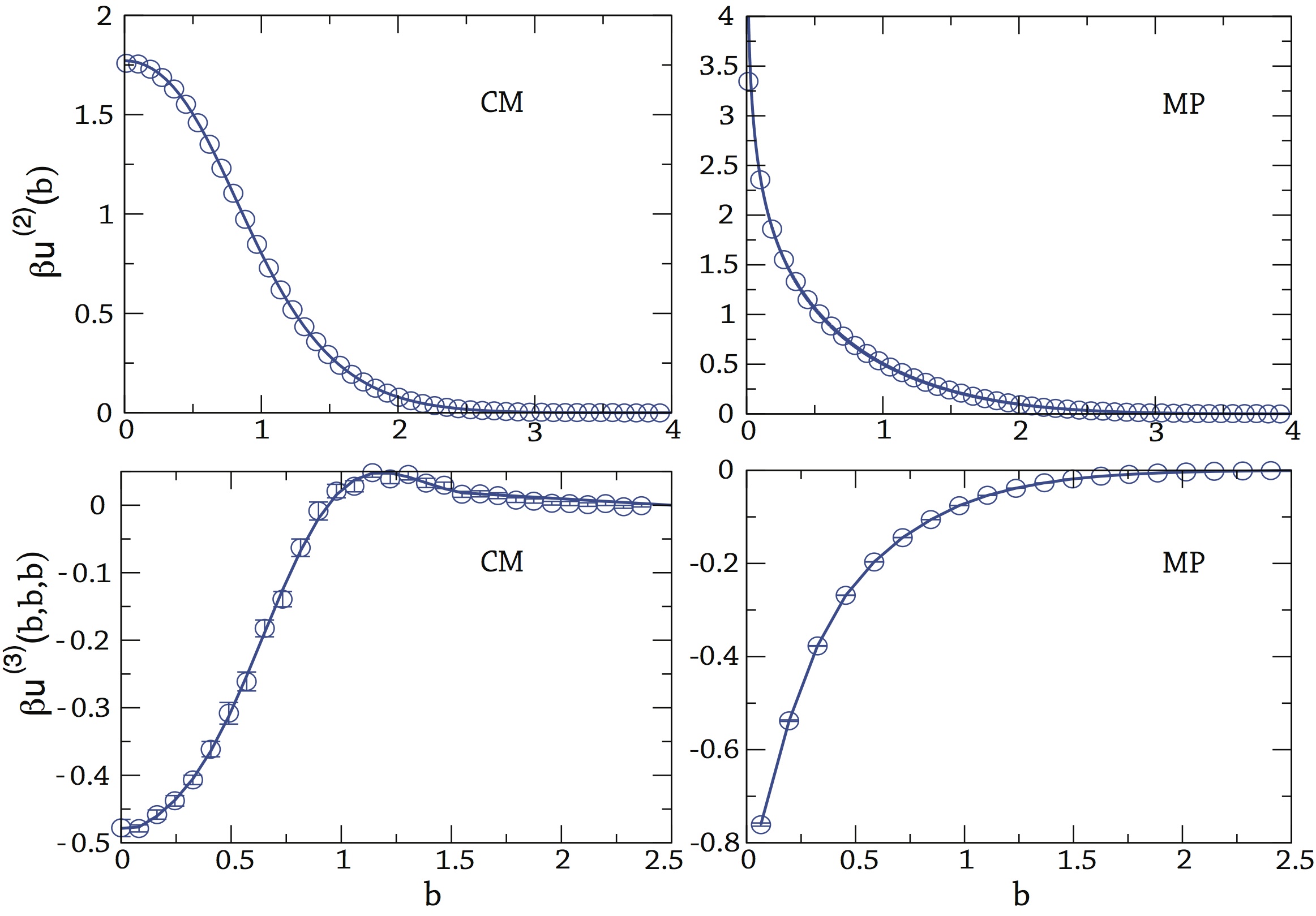
Figure 1: Top: Effective pair potential $u^{(2)}(b)$ in the CM (left) and MP (right) representations as a function of $b=r/R_{g}$. We report (circles) numerical DJ results and (full lines) the corresponding parametrizations (11) and (12). Bottom: Effective three-body potential $\beta u^{(3)}(b,b,b)$ as computed in the CM and MP representations as a function of $b=r/R_{g}$. The simulation results (squares) are obtained by means of Monte Carlo simulations of the DJ model. The full lines are only meant to guide the eye. For the CM representation, DJ results agree with those obtained by using the SAW model BLH-01 ; PH-05 , as expected on the basis of universality.

The determination of $u^{(3)}$ requires the computation of a triplet correlation, a function of three independent scalar variables, which is a cumbersome simulation task. Therefore, we only show results for polymer configurations whose CG sites are on the vertices of an equilateral triangle of side $b$. The simulations results for the DJ model are reported in Fig. 1. While in the MP representation the effective potential is purely attractive and diverging to $-\infty$ as $\rho\to 0$ (a result that can be proved on general grounds vonFerber-etal-2 ; Pelissetto-12 ), in the CM representation it is soft, attractive at short distance ($\rho<1$), and with a small repulsive tail for $\rho>1$. For the CM representation, four-body and five-body were also determined BLH-01 , at least for some particular polymer configurations. In particular, at least up to $n=5$, it was found that the generic $n$-body potential at small distances is positive (repulsive) for even $n$’s and negative (attractive) for odd $n$’s. Moreover, the strength of the $n$-body potential at small distances decreases for increasing $n$. For the MP representation this behavior was proved for all values of $n$ and generic star polymers with $f$ arms Pelissetto-12 : moreover, it was shown that the $n$-body potential at full overlap $b_{1}=\ldots=b_{n}=0$ decreases logarithmically, at least for star polymers with a large number of arms.

The full computation of the many-body terms is very difficult and of little practical use, since numerical simulations of the model using three-body or higher-order interactions would be unfeasible. Indeed, the computational cost grows as $N^{n}$, where $n$ is the largest order included and $N$ is the number of constituents of the system. Therefore, in most of the applications the many-body expansion is truncated, considering only the zero-density pair potential of mean force (6). It is therefore important to quantify the accuracy of this very simplified effective model.

As a first check of its accuracy, we consider the universal third-virial combination $A_{3}=B_{3}/R_{g}^{6}$, which depends explicitly on the three-body interaction term, see Eq. (9). Thus, comparison of $A_{3}$ computed in the FM model with the value computed in the CG model provides us with a direct estimate of the quantitative relevance of the neglected three-body interactions. For polymers in the scaling limit $A_{3}=9.90(2)$ CMP-06 . Using Eq. (9) with $u^{(3)}=0$ and parametrizations (11) and (12) we obtain instead $A_{3,CM}=7.85$ and $A_{3,MP}=4.92$ for the two different representations. The CG model underestimates the FM value $A_{3}=9.90(8)$ in both cases: by $21\%$ in the CM case and by $50\%$ in the MP case, respectively. This shows that three-body interactions are relevant: if they are neglected, the pressure may be significantly underestimated. Similar conclusions are reached by directly comparing the equation of state. A simple estimate of $Z=\beta\Pi/\rho$, $\rho=N/V$, for the CG system can be obtained by using the random-phase approximation (RPA) HMD-06 , which is expected to be accurate for systems with soft potentials and becomes exact for large densities. If $\Phi=(4\pi R_{g}^{3}\rho)/3$, it predicts

$$Z_{RPA,CM}=1+1.71\Phi,$$

$$Z_{RPA,MP}=1+1.54\Phi.$$ (14)

Clearly, the CG model does not capture the correct scaling of the osmotic pressure in the semidilute regime, i.e., $Z\propto\Phi^{1.309}$ deGennes-79 ; dCJ-book , underestimating the correct result. Moreover, $Z$ depends on the chosen CG representation, a dependence which would be absent in the exact mapping. In particular, consistently with the results for $A_{3}$, the osmotic pressure in the CM representation is always larger than the MP representation estimate.

More quantitatively, we can compare the compressibility factor $Z$ in a wide range of densities, representative of both the dilute and semi-dilute regimes. In Table 1 we report FM results Pelissetto-08 and estimates obtained by using the CG models. In the latter case, we show both simulation results and estimates obtained by using integral-equation methods with the HNC closure (they are fully consistent in the whole density range, confirming the accuracy of the HNC closure for soft potentials). The CG model based on the CM representation appears to be more accurate than that based on the MP representation. However, both approaches show significant deviations from the correct FM estimates in the semidilute regime. This can be easily understood. For $\Phi$ larger than 1, polymers overlap, so that many-body interactions, neglected in the simple CG model with pair potentials, play a relevant role.

Table 1: Compressibility factor $Z(\Phi)=\beta\Pi/\rho$ for polymers (FM) in the scaling limit Pelissetto-08 and for the CG model in the center-of-mass (CM) and in the mid-point (MP) representation. Both HNC and Monte Carlo (MC) predictions are reported.

$\Phi$	FM	CM-MC	CM-HNC	MP-MC	MP-HNC
0.135	1.187	1.18458(1)	1.185	1.17869(1)	1.182
0.27	1.393	1.38167(1)	1.382	1.36439(1)	1.371
0.54	1.854	1.80067(1)	1.803	1.74840(1)	1.762
0.81	2.371	2.23911(1)	2.241	2.14190(1)	2.162
1.09	2.959	2.70461(1)	2.707	2.55534(1)	2.582
2.18	5.634	4.55607(2)	4.559	4.18703(1)	4.240
4.36	12.23	8.29709(2)	8.303	7.47886(3)	7.584

The results presented so far are relative to polymers under good-solvent conditions. The CG strategy can be extended to describe solutions in the thermal crossover region towards the $\theta$ point, as well DPP-13-thermal . Indeed, universality holds even in this intermediate regime if properties are expressed in terms of the polymer volume fraction $\Phi$ and of the Zimm-Stockmayer-Fixman ZSF-53 $z$-variable, $z\propto(T-T_{\theta})L^{1/2}$, which combines the deviation of the temperature from the $\theta$ value and the chain length $L$, as long as logarithmic corrections (which are relevant at the $\theta$ point) are neglected deGennes-79 ; dCJ-book ; Schaefer-99 . Equivalently, and with a more direct physical meaning, the $z$-variable can be replaced by the second-virial combination $A_{2}$, whose functional dependence on $z$, $A_{2}(z)$, has been fully characterized in Ref. CMP-08 . When approaching the good-solvent regime, we have $z\to\infty$ and $A_{2}(\infty)=5.500(3)$, while, when approaching $T_{\theta}$, $z\to 0$ and $A_{2}(z)\approx 4\pi^{3/2}z$. In Ref. DPP-13-thermal it has been shown that the CG single-site model with zero-density pair potentials becomes accurate in an increasingly large density range when approaching the $\theta$ point. This can be explained by noting the the $n$-th order virial coefficient scales as $z^{n}$ for $z\to 0$, so that $n$-body terms become increasingly less relevant approaching the $\theta$ point.

The model discussed in Ref. DPP-13-thermal neglects logarithmic corrections that scale as $1/\ln L$, hence vanish in the critical limit, but which may be relevant for finite values of $L$. Apparently, they can be neglected when considering the second virial coefficient or the expansion ratio that gives the variation of the radius of gyration as solvent quality changes PCP-suppl ; PIB-suppl ; PS-suppl (see also the supplementary material of Ref. DPP-14-GFVT for an extensive discussion). However, for some different quantities they are relevant: for instance, they determine the deviations from the ideal behavior of the equation of state at the $\theta$ point in the semidilute regime and the peculiar behavior of the third virial coefficient NNT-91-suppl ; ANNT-94-suppl ; PH-05 . Unfortunately, it is not possible to use CG models to account also for these logarithmic corrections. Indeed, at the $\theta$ point the CG model with only pair potential is not thermodynamically stable KHL-03 ; AJH-04 ; PH-05 .

III State-dependent interactions

III.1 General theory

To enlarge the density range in which CG single-site models with pairwise effective interactions can be used, one strategy proposed in the past is based on deriving and using state-dependent interactions. Structurally derived state-dependent potentials have been mostly discussed in the context of the canonical ensemble, see Refs. SST-02 ; Louis-02 ; JHGL-07 ; DPP-13-state-dep and references therein, hence all thermodynamic and structural quantities depend on the density $\rho$. In this approach the pair potential $u^{(2)}(r;\rho)$ is obtained by requiring the CG model to reproduce the two-point correlation function ${\cal G}^{(2)}(r;\rho)$ at the given value of the density. The uniqueness of such a potential is guaranteed by Henderson’s theorem Henderson-74 ; CCL-84 . Of course, for $\rho\to 0$ the potential $u^{(2)}(r;\rho)$ converges to the potential of mean force $u^{(2)}(r)$ considered before. The inversion of ${\cal G}^{(2)}(r,\rho)$ to extract $u^{(2)}({r};\rho)$ can be performed by means of iterative procedures. For instance, one could use the iterative Boltzmann inversion method MullerPlathe-02 . For soft potentials the HNC inversion schemeBL-02 ; BLHM-01 is also particularly convenient.

Although use of $u^{(2)}(r;\rho)$ allows one to reproduce the pair distribution function for any value of the density, there is no warranty that any other structural property of the underlying system—for instance, the three-body correlation function—is reproduced correctly. Moreover, state-dependent interactions introduce some inconsistencies in the calculation of standard thermodynamic properties Louis-02 ; SST-02 ; DPP-13-state-dep . For instance, in systems with state-independent potentials there are two equivalent routes to the pressure. One can define it mechanically (virial pressure), as the force per unit area acting on the boundaries, or thermodynamically, as the derivative of the free energy with respect to density. In the presence of state-dependent interactions the two definitions are no longer equivalent Louis-02 ; DPP-13-state-dep . Moreover, in the case of density-dependent potentials none of them reproduces the correct pressure of the underlying system, although, at least in the low-density limit, the virial expression is closer to the correct pressure than the thermodynamic one DPP-13-state-dep . Another problem of the approach is that effective state-dependent potentials depend on the ensemble in which they have been derived DPP-13-state-dep : the equivalence of the ensembles breaks down. Therefore, different thermodynamic results are obtained by using CG models defined at the same state point of the underlying system but in different ensembles, making the computation of phase transitions and transition lines quite challenging. As a general message, care is needed when using state-dependent interactions to derive the thermodynamics of the original system and to compute free energies. In particular, one should be careful to employ state-dependent potentials only in the statistical ensemble in which they have been derived.

III.2 Homopolymer solutions

To elucidate the issues related to the use of state-dependent interactions, we consider again CG single-site models for linear homopolymers under good-solvent condition. This case, in the CM representation, has been discussed extensively in the past and a complete comparison between the underlying FM system and the CG model, mainly focused on thermodynamic, interfacial and large-scale structural properties, has been reported in Refs. LBHM-00 ; BLHM-01 ; BL-02 . In particular, Ref. BL-02 reports an explicit parametrization of the density-dependent pair potential obtained by matching the CM-CM pair distribution function for SAWs with $L=500$ monomers. Since interactions are soft and the CG model corresponds to a monoatomic liquid, the inversion procedure was performed by using an integral-equation method with the HNC closure. This method requires a minimal computational effort and provides accurate estimates of the thermodynamic behavior.

In Fig. 2 we report the effective pair potential $u^{(2)}(b;\Phi)$ (CM representation) for linear polymers at $\Phi=0,0.4,1$ obtained by using the HNC inversion procedure. The associated $g^{(2)}(b;\Phi)$ has been computed by FM simulations of the DJ model with polymers of length $L=2400$. At first glance, the potentials appear to be not very sensitive to the polymer volume fraction. The value at full overlap increases slightly with density in the range of polymer volume fractions under consideration. For larger concentrations the strength of the interaction decreases again LBHM-00 ; BLHM-01 , as a consequence of the screening of the excluded-volume interaction. Moreover, the potential has a slightly longer range compared to the zero-density case, ensuring the correct scaling behavior of the osmotic pressure in the semi-dilute regime. The accuracy of the inversion can be tested by performing Monte Carlo simulations of the CG model and comparing the resulting pair distribution functions with those used as targets in the inversion procedure. From the results shown in Fig. 2 we can conclude that the HNC inversion for the CM representation is an accurate way to provide structurally consistent effective pair potentials.

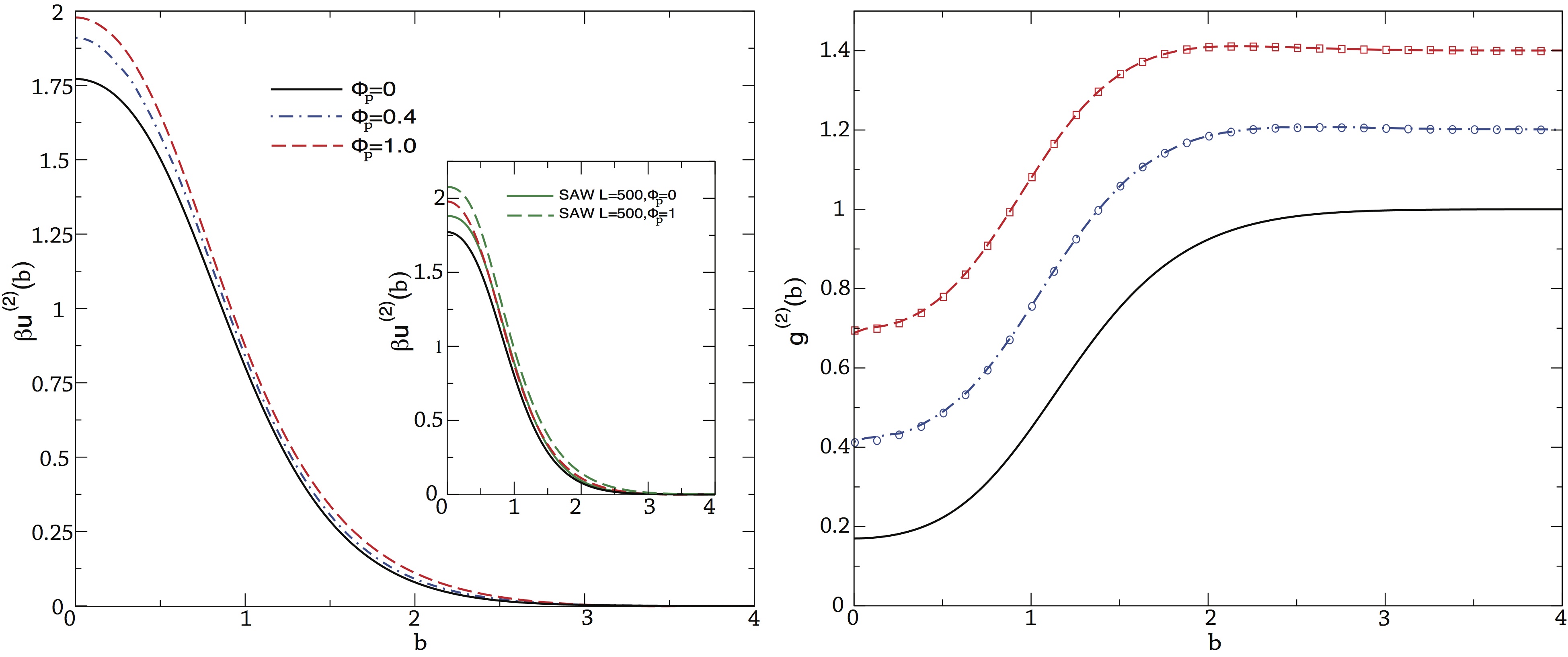
Figure 2: Left panel: Effective pair potential $u^{(2)}(b;\Phi)$ for different densities, $\Phi=0,\Phi=0.4,\Phi=1$, as obtained by HNC inversion (CM representation). In the inset we compare the effective potentials obtained in the scaling limit with those appropriate for SAWs with $L=500$ sites. Right panel: Radial distribution functions between the polymer CMs as obtained by Monte Carlo simulations of the FM model (lines) and of the CG model with density-dependent potential (squares and circles) for $\Phi=0.4$ and $\Phi=1$. We also report the zero-density distribution function (full line). Data for $\Phi=0.4$ and $\Phi=1$ are shifted upward for clarity.

The results for the effective potentials reported in Ref. BL-02 differ somewhat from those we have determined by using long DJ chains, which effectively provide results in the scaling limit. The reason is that in Ref. BL-02 finite-length SAWs ($L=500$) were considered, without performing a scaling-limit extrapolation. SAW results are affected by relatively large scaling corrections, which increase with density (for a discussion, see Ref. Pelissetto-08 ), even when $L$ is of order $10^{3}$. In the zero-density limit, scaling corrections are clearly visible in the result for the pair potential, which is somewhat more repulsive than the accurate expression (11), obtained by performing a proper extrapolation to the limit $L\to\infty$. In particular, the value at full overlap ($b=0$) of the potential exceeds the asymptotic one by $6\%$. A similar difference is observed for the second virial coefficient, which takes the value 6.18 if one uses the potential of Ref. BL-02 , to be compared with the value $5.50(3)$ obtained in the scaling limit CMP-06 . To further test the accuracy of the potential, we have determined the potential at $\Phi=1$ by using the pair distribution function obtained from simulations of the DJ model, finding again a discrepancy of approximately $6\%$ for the value at full contact, see Fig. 2.

Now we analyze the consistency of the results obtained by using state-dependent interactions. For this purpose, we consider SAWs with $L=500$ as our underlying system, so that we can use the effective density-dependent potentials reported in Ref. BL-02 , which apply to a large $\Phi$ interval, up to $\Phi=2.5$. Then, we determine the chemical potential using three different routes, that are equivalent for systems with state-independent interactions. We report results for

$$\beta\hat{\mu}=\ln(\rho R^{3}_{g})+\beta\mu^{(\rm exc)},$$ (15)

which differs from the correct chemical potential by an irrelevant, model dependent constant, but which has the advantage of being universal. First, we consider the HNC expression for the chemical potential Morita-60 ; Attard-91 (HNC-route)

$$\beta\hat{\mu}_{\rm HNC}(\Phi)=\ln{\left(\frac{3}{4\pi}\Phi\right)}+\frac{3}{4\pi}\Phi\int d^{3}{\bm{b}}\left[h(b)^{2}-h(b)c(b)-2c(b)\right],$$ (16)

where $h(b)=g^{(2)}(b;\Phi)-1$ and the direct correlation function $c(b)$ is related to $\Phi$ and $h(b)$ by the Ornstein-Zernike relation HMD-06 :

$$h(b_{1})=c(b_{1})+(3\Phi/4\pi)\int d{\bm{b}}_{2}c(b_{2})h(b_{12}),$$ (17)

where $b_{12}=|{\bm{b}}_{1}-{\bm{b}}_{2}|$. A second possibility consists in determining first the compressibility factor $Z=\beta\Pi/\rho$ by means of the virial expression,

$$Z_{\rm vir}(\Phi)=1-{8\pi^{2}\over 9\Phi}\int_{0}^{\infty}{\partial\beta u^{(2)}(b;\Phi)\over\partial b}g^{(2)}(b;\Phi)b^{3}db,$$ (18)

and then in computing $\hat{\mu}$ as (Z-route)

$$\beta\hat{\mu}_{Z}(\Phi) = \ln\left(\frac{3}{4\pi}\Phi\right)+Z_{\rm vir}(\Phi)-1+\int_{0}^{\Phi}\frac{Z_{\rm vir}(\xi)-1}{\xi}d\xi.$$ (19)

Finally, we consider the compressibility route (K-route), which is based on

$$\beta\hat{\mu}_{K}(\Phi)=\ln{\left(\frac{3}{4\pi}\Phi\right)}+\int_{0}^{\Phi}\frac{K(\xi)-1}{\xi}d\xi,$$ (20)

with $K(\Phi)$ given by

$$K(\Phi)^{-1}=1+\frac{3}{4\pi}\Phi\int d^{3}{\bm{b}}\left[g^{(2)}(b;\Phi)-1\right].$$ (21)

For CG models with density-dependent interactions, only the K-route provides the correct chemical potential of the underlying model Louis-02 ; DPP-13-state-dep . Indeed, since the CG procedure reproduces the pair distribution function at any density, $K(\Phi)$, defined in Eq. (21), is the same in the CG and in the underlying model. Hence, also $\beta\hat{\mu}_{K}(\Phi)$ defined in Eq. (20) is the same. Note also that, the Z-route and the K-route both require the effective potential to be computed for all densities smaller than the physical density of interest, hence they have a limited predictive power.

Table 2: Polymer chemical potential $\beta\hat{\mu}$ computed in the density-dependent CG model appropriate to describe $L=500$ SAWs (we use the parametrization of the effective pair potential reported in Ref. BL-02 ). We report results using three different routes (the HNC-route, the Z-route, the K-route), as discussed in the text, and the expression reported in Ref. FBD-08 (FBD). The results labelled “FM scaling” are obtained by using the FM, scaling-limit equation of state reported in Ref. Pelissetto-08 .

$\Phi_{p}$	HNC-Route	Z-route	K-route	FBD	FM scaling
0.25	$-$1.98	$-$2.02	$-$2.03	$-$1.99	$-$2.11
0.5	$-$0.26	$-$0.36	$-$0.43	$-$0.28	$-$0.62
1.0	3.07	2.77	2.43	3.06	1.89
1.5	6.83	6.14	5.41	6.80	4.35
2.	11.00	9.80	8.59	10.96	6.90
2.5	15.28	13.73	11.98	15.42	9.55

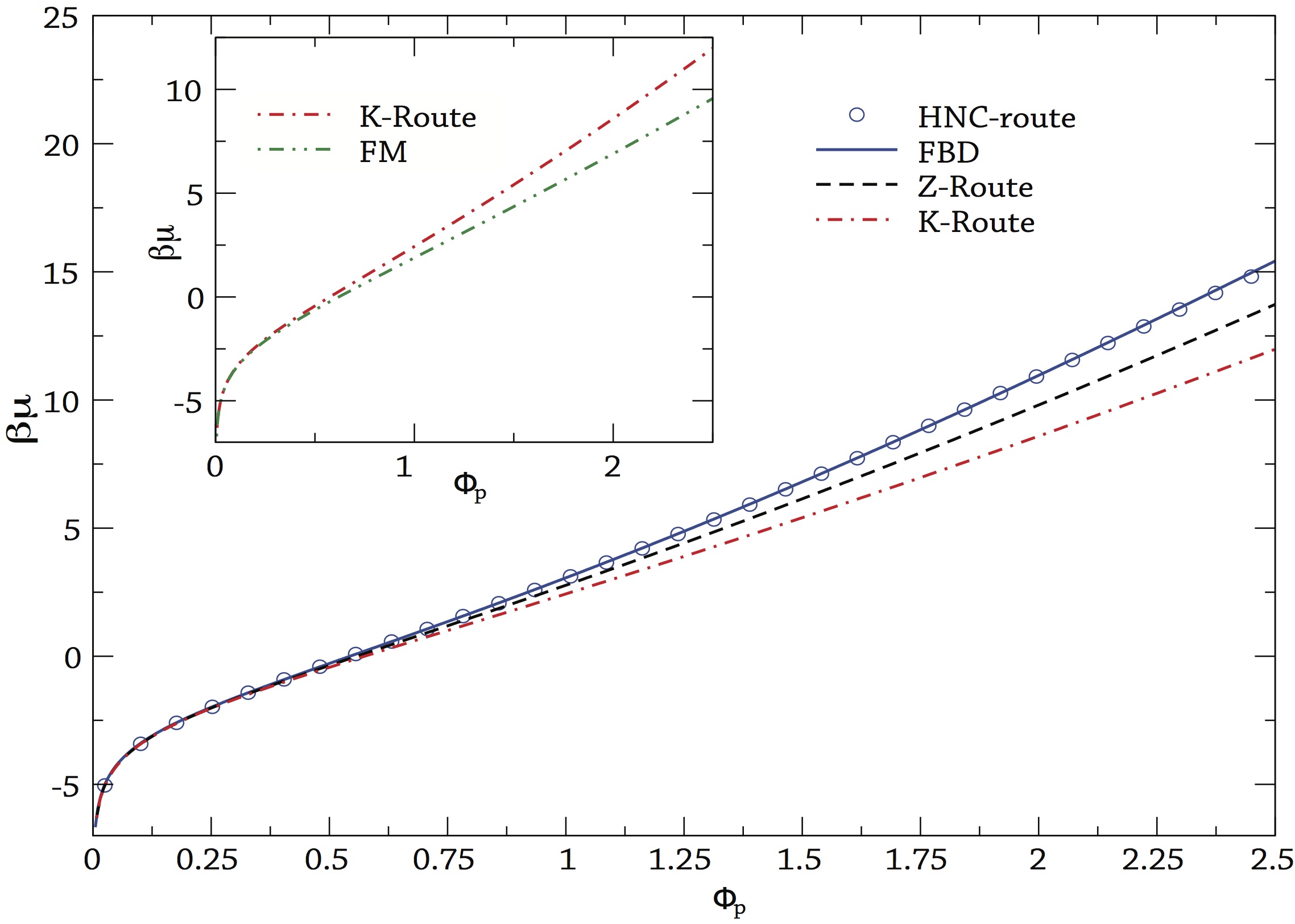
Figure 3: Polymer chemical potential $\beta\hat{\mu}$ computed in the density-dependent CG model appropriate to describe $L=500$ SAWs (we use the parametrization of the effective pair potential reported in Ref. BL-02 ). We report results using three different routes (the HNC-route, the Z-route, the K-route), as discussed in the text, and the expression reported in Ref. FBD-08 (FBD) In the inset we compare the results using the K-route (which are the same as those computed directly by using $L=500$ SAWs) and the analogous results obtained by using the FM, scaling-limit equation of state reported in Ref. Pelissetto-08 .

Results are reported in Table 2 and in Fig. 3. It is apparent that inconsistencies between the different routes, well beyond the degree of inaccuracy related to the use of the HNC method, are present even in the dilute regime. The three different routes provide different predictions, satisfying $\beta\hat{\mu}_{\rm HNC}>\beta\hat{\mu}_{Z}>\beta\hat{\mu}_{K}$ for all the densities under consideration. As a consequence, since the K-route estimate agrees with the chemical potential of the underlying system, the HNC-route and the Z-route both overestimate the correct chemical potential. It is interesting to observe that the HNC-route results are equivalent (with a small error due to HNC approximation) to those that would be obtained in a direct canonical Monte Carlo simulation by employing Widom insertion method Widom-63 , i.e., this route corresponds to the estimate that would be obtained in the approach referred to as passive approach in Ref. DPP-13-state-dep . In other words, the HNC-route result is the one that would be obtained by using standard thermodynamic relations, disregarding the density dependence of the potential. As a consequence, ensemble equivalence is satisfied. If one performs grand-canonical simulations at chemical potential $\beta\hat{\mu}_{\rm HNC}(\Phi)$ with potential $u^{(2)}(b;\Phi)$, one obtains the correct volume fraction $\Phi$. However, the fact that ensemble equivalence is satisfied is completely unrelated to the question whether $\beta\hat{\mu}_{\rm HNC}(\Phi)$ is a correct estimate of the chemical potential of the underlying system. Indeed, as our results show, $\beta\hat{\mu}_{\rm HNC}(\Phi)$ differs significantly from the correct result. Finally, it is interesting to compare $\beta\hat{\mu}_{K}$ obtained here (which gives the correct chemical potential for $L=500$ SAWs) with the chemical potential that is obtained by using the equation of state of Ref. Pelissetto-08 , which refers to polymers in the scaling limit. The two quantities are reported in the inset of Fig. 3. The SAW model clearly overestimates the scaling-limit result, deviations significantly increasing with $\Phi$.

IV Single-site coarse-grained model for multicomponent systems

In this section we generalize the discussion of Sec. II to multicomponent systems. In particular, we focus on colloidal dispersions comprising large particles, colloids, usually modeled as hard spheres, and polymers in an implicit solvent. These systems are particularly interesting as they show a complex phase diagram which depends crucially on the polymer-to-colloid size ratio: for small ratios, only fluid-solid coexistence is observed, while for larger values an additional fluid-fluid transition is present Poon-02 ; FS-02 ; TRK-03 ; MvDE-07 ; FT-08 ; ME-09 . Even in the absence of an explicit solvent, the computation of the full phase diagram is quite difficult, especially if one is interested in polymers with a large degree of polymerization. Therefore, CG models represent an important tool to investigate these systems. A first class of CG model is obtained by integrating out all polymer degrees of freedom. The resulting CG system is a one-component model of colloids interacting via an effective potential. Repeating the discussion of Sec. II.1, one obtains an effective potential with an infinite number of many-body terms. Computationally it is unfeasible to include more that the leading, two-body term. However, such a truncated model is only predictive when the polymer-to-colloid size ratio is small. A less extreme approach consists in integrating out only the internal degrees of freedom of the polymer, representing each macromolecule with a monoatomic molecule, as already discussed in Sec. II.2. After this reduction, one obtains a two-component system, comprising colloids and monoatomic CG polymers, which can be studied with much more ease than the original system.

Two-component single-site CG models have been considered in several papers BLH-02 ; Dzubiella-etal-01 ; DLL-02 ; SDB-03 ; VJDL-05 ; PH-06 ; ZVBHV-09 ; AP-12 and also discussed in Ref. DPP-14-GFVT . Here, we shall only discuss models in which pair potentials are determined accurately by using FM data, in order to assess the reliability of the single-site model with pairwise interactions (other results are summarized and discussed in Ref. DPP-14-GFVT ). In Refs. DPP-13-depletion ; DPP-14-colloidi we performed a careful comparison, considering both the model defined at zero-density and that using potentials depending on the polymer density BLH-02 , focusing on the solvation properties of a single colloid in a polymer solution and on the thermodynamics in the homogeneous phase. As expected, the model is only accurate if $q=R_{g}/R_{c}$ is less than 1 ($R_{c}$ is the radius of the colloid). The failure of the model when polymers are larger than colloids can be understood physically, by noting that, when $q>1$, polymers can wrap around the colloids, a phenomenon that cannot be modelled correctly if polymers are represented as soft spheres. Moreover, the system is accurate only if the polymer volume fraction $\Phi_{p}=4\pi R_{g}^{3}\rho_{p}/3$ (to avoid confusion with colloidal quantities, we add a suffix “$p$” to all polymer-related quantities) is less than 1, guaranteeing that the neglected three-polymer interactions are small. Finally, the accuracy decreases with increasing colloid volume fraction $\Phi_{c}=4\pi R^{3}_{c}\rho_{c}/3$ ($\rho_{c}=N_{c}/V$ is the colloid density), since the relevance of the polymer-many-colloid interactions increases in this limit.

Here we discuss the phase diagram of polymer-colloid solutions as predicted by CG single-site models. To assess their accuracy we need reference results to compare with. For $q=1$ we will use FM results CVPR-06 ; MLP-12 ; MIP-13 . To the best of our knowledge, there are no such results for $q<1$, hence we will compare our Monte Carlo estimates for the CG model with the binodals obtained by using the generalized free-volume theory (GFVT) FT-08 ; ATL-02 ; FT-07 ; TSPEALF-08 ; LT-11 ; DPP-14-GFVT , which is expected to become increasingly accurate as $q$ decreases.

We consider three values of $q$, $q=0.5$, 0.8, and 1. For the CG models with zero-density and density-dependent interactions, we perform standard grand-canonical simulations using a recursive umbrella-sampling algorithm TV-77 ; PRT-14 . Insertions and deletions of colloids and polymers are performed by using the cluster moves introduced by Vink and Horbach VH-04 ; Vink-04 , which considerably improve the performance of the simulation. Simulation parameters are the fugacities $z_{p}$ and $z_{c}$, which are normalized so that $\rho_{p}R_{g}^{3}=z_{p}$ and $\rho_{c}R_{c}^{3}=z_{c}$ for $\rho_{p},\rho_{c}\to 0$. Instead of $z_{c}$ we shall usually quote $\beta\mu_{c}=\ln z_{c}$, while, as often in the literature, instead of reporting $z_{p}$, we will report the volume fraction $\Phi_{p}^{(r)}$ of a polymer reservoir at the same value of $z_{p}$. For the zero-density CG model the reservoir volume fraction can be obtained by inverting the corresponding equation of state ($z_{p}=e^{\beta\hat{\mu}_{p}}$) which we have parametrized as:

$$Z(\Phi_{p}) = {(1+6.05117\Phi_{p}+11.6052\Phi_{p}^{2}+10.2588\Phi_{p}^{3})^{1/2}\over(1+3.42865\Phi_{p})^{1/2}}$$ (22)

$$\beta\hat{\mu}_{p}(\Phi_{p}) = \ln\left(\frac{3}{4\pi}\Phi_{p}\right)+Z(\Phi_{p})-1+\int_{0}^{\Phi_{p}}\frac{Z(\xi)-1}{\xi}d\xi.$$ (23)

IV.1 Results for $q=1$

Before studying phase separation by using the CG model, we have determined the reference binodal, using the FM results of Ref. MLP-12 . Given the computational complexity of the system, the simulated chains are relatively short. Therefore, the results of Ref. MLP-12 show significant corrections to scaling, which should be taken into account before any comparison with the CG results. The scaling-limit binodal curve can be obtained by extrapolating the data of Ref. MLP-12 , along the lines of the critical-point extrapolation performed in Ref. DPP-14-GFVT . In Sec. IV.B of Ref. DPP-14-GFVT we considered the estimates of the critical points $\Phi_{c,\rm crit}(L)$ and $\Phi_{p,\rm crit}(L)$, for three systems with $L=10,33,110$ and approximately $q=1$, and determined the critical point in the scaling limit. We obtained DPP-14-GFVT : $\Phi_{c,\rm crit}(\infty)\approx 0.22$ and $\Phi_{p,\rm crit}(\infty)\approx 0.62$. Analogously, if $\Phi_{p}^{\rm bin}(L,\Phi_{c})$ gives the position of the binodal for the system with chains of length $L$, we fit the data to

$$\Phi_{p}^{\rm bin}(L,\Phi_{c})\approx\Phi_{p}^{\rm bin}(\Phi_{c})+\frac{a_{1}(\Phi_{c})}{\sqrt{L}}.$$ (24)

The curve $\Phi_{p}^{\rm bin}(\Phi_{c})$ is our estimate of the scaling-limit binodal. Another possibility, although less rigorous, is to rescale, for each value of the length $L$, the finite-$L$ binodal so as to obtain the correct critical point. In other words, we set

$$\Phi_{p}^{\rm bin}(\Phi_{c})=a\Phi_{p}^{\rm bin}(L,b\Phi_{c})$$ (25)

with

$$a={\Phi_{p,\rm crit}(\infty)\over\Phi_{p,\rm crit}(L)}\qquad b={\Phi_{c,\rm crit}(L)\over\Phi_{c,\rm crit}(\infty)}.$$ (26)

The binodals computed with this method turn out to be essentially independent of the value of $L$, supporting the method, and quite close to that computed by direct extrapolation. The different extrapolations are reported in Fig. 4, together with the corresponding finite-$L$ results.

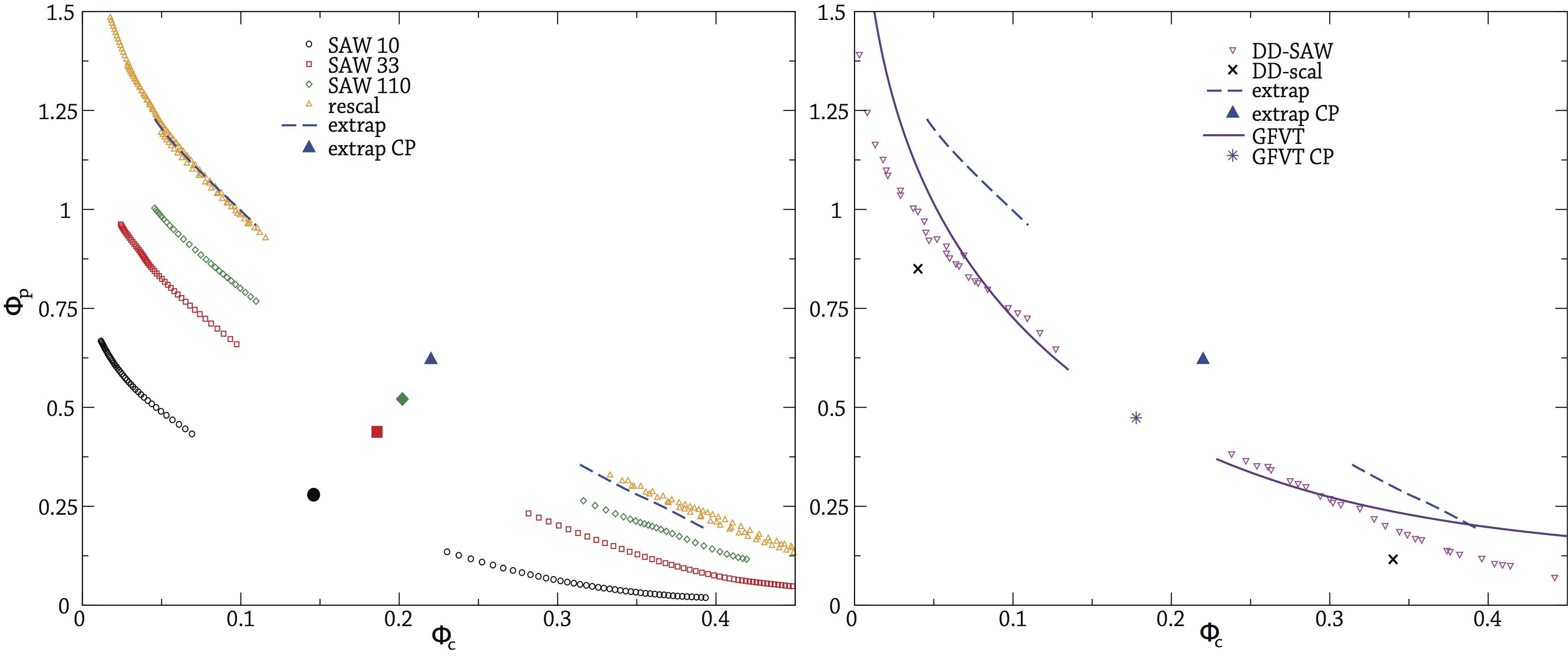
Figure 4: Left: binodal curves for $q=1$ obtained by using the results of Ref. MLP-12 . We report the finite-$L$ data ($L=10$, $L=33$, $L=110$), the extrapolation obtained by using Eq. (24) (”extrap”), and the binodal obtained by the simple rescaling mentioned in the text (”rescal”) starting from the results with $L=110$. CP is the extrapolated critical point. Right: We report the FM binodal (extrap), the GFVT prediction, and that obtained in Ref. BLH-02 using polymer-density-dependent potentials appropriate for $L=500$ SAWs (DD-SAW). We also report two points (crosses,DD-scal) belonging to the binodal obtained using polymer-density-dependent potentials appropriate for scaling-limit polymers. We also report the corresponding critical points (CP).

Once the reference binodal was determined, we considered the single-site CG model with zero-density potentials. We systematically increased $z_{p}$ and for each value of this parameter we performed several runs with different values of $z_{c}$, covering colloid volume fractions from 0.1 to 0.35. In all cases no sign of coexistence was observed for systems of size $V=(17.7\ R_{g})^{3}$. Of course, one might fear that systems are too small to allow us to identify a phase transition. Therefore, we repeated the analysis using integral-equation methods. We considered the binary system and used the HNC closure for all correlations. Again, no sign of phase separation was observed.

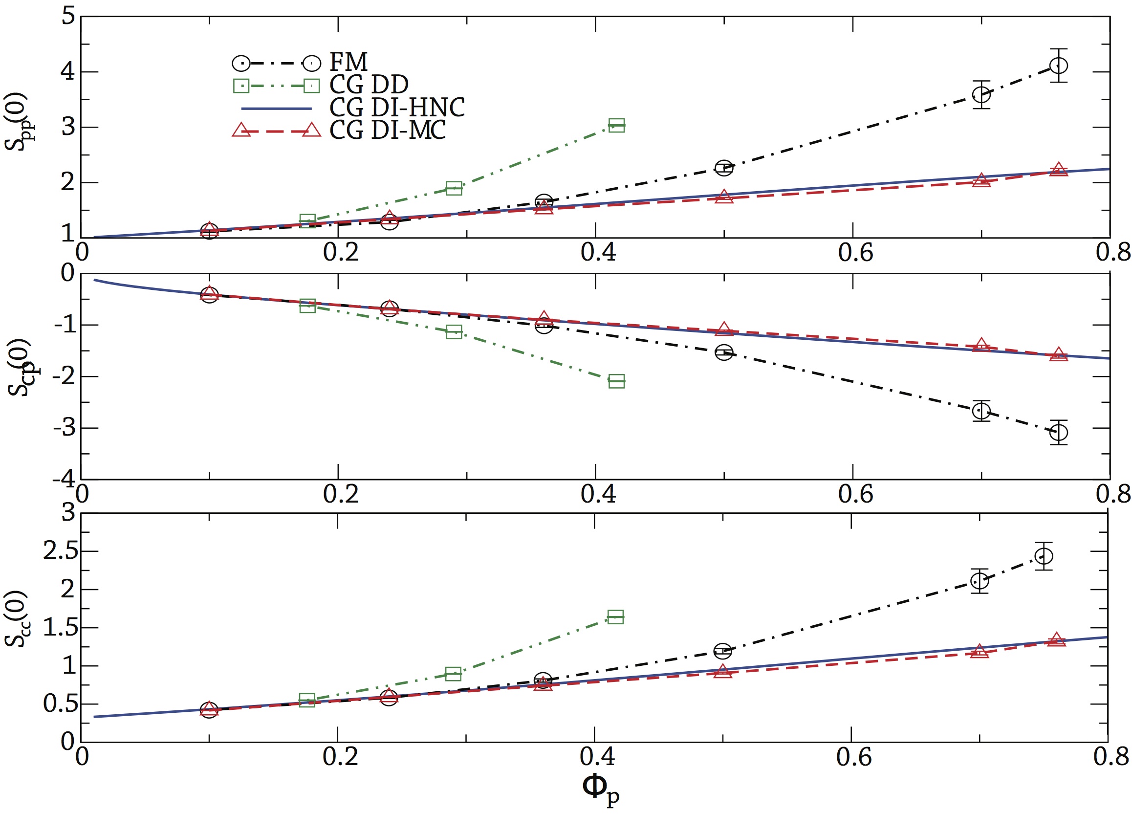
Figure 5: Partial structure factors at $k=0$ as a function of $\Phi_{p}$ for $\Phi_{c}=0.15$. We report full-monomer (circles, FM) results obtained by using DJ chains of length $L=2400$, CG results obtained by using the zero-density model [Monte Carlo results (triangles, CG DI-MC) and HNC results (lines, CG DI-HNC)], and by using the density-dependent model (squares, CG DD).

The evidence of a wide region of stability of the homogeneous phase, well beyond the full-monomer phase boundaries, is surprising. Indeed, one does not expect the single-site model to be accurate if colloids and polymers have the same size, hence quantitative differences are not surprising. The unexpected feature is that the CG model is not even able to predict the qualitative behavior of the system.

To understand why the CG model does not show phase separation, we have determined the partial structure factors $S_{\alpha\beta}(k)$ ($\alpha,\beta=p,c$) and determined their limiting value for $k\to 0$. Such quantities are indeed order parameters of the fluid-fluid transition. We have determined these quantities for the DJ model with chains of length $L=600$ and for the CG model for $\Phi_{c}=0.15$ and several values of $\Phi_{p}$. For the CG model we have determined the structure factors both numerically, by performing Monte Carlo simulations, and by using integral-equation methods (we use the HNC closure) on very large systems $V=(64R_{g})^{3}$. Results are reported in Fig. 5. For small polymer volume fractions, the CG and DJ results are in full agreement, but, as $\Phi_{p}$ increases, the CG model significantly underestimates the structure factors. At coexistence, which should occur for $\Phi_{p}\approx 0.7$-0.8, the FM estimates are $S_{pp}(0)\approx 4$, $S_{cc}(0)\approx 2.5$, which are significantly larger than the CG estimates. More precisely, for $\Phi_{p}=0.76$ we obtain $S_{pp}(0)=4.1$ and 2.3 for the DJ and the CG model, respectively. For $S_{cc}(0)$, we obtain correspondingly $S_{cc}(0)=2.2$ (DJ) and 1.3 (CG). If we further increase $\Phi_{p}$, the CG results change only slightly. We obtain $S_{pp}(0)=2.5$ and $S_{cc}(0)=1.5$ for $\Phi_{p}=1.0$. Clearly, even increasing polymer density the system appears to be unable to develop long-range correlations.

The results for the CG model are in contrast with those of Ref. BLH-02 , which observed phase coexistence for $q=1$, using the model with density-dependent interactions. Quantitatively, the binodal obtained in Ref. BLH-02 differs somewhat from that obtained by using the FM estimates, see Fig. 4. The results for Ref. BLH-02 refer to SAWs with $L=500$ monomers, hence one might fear that the differences between the CG and the full-monomer results are due to the different reference system. To clarify the issue, we have redetermined the density-dependent potential for $\Phi_{p}^{(r)}=1$ using scaling-limit FM data and recomputed the position of the binodal for such a value of $\Phi_{p}^{(r)}$. We find coexistence between $(\Phi_{c},\Phi_{p})=(0.04,0.86)$ and $(0.34,0.12)$. These two points are also reported in Fig. 4. They show that the scaling-limit binodal computed by using the density-dependent potential is not very different from that computed by Ref. BLH-02 and still significantly below the FM binodal. It is interesting to note that the GFVT binodal is essentially on top of the binodal of Ref. BLH-02 . In view of the previous discussion, however, such an agreement looks accidental.

To understand why the CG model with density-dependent potentials predicts phase separation, we have computed also in this case the partial structure factors. They are shown in Fig. 5. It is clear that the model with zero-density potential provides a better approximation to the FM results than that using density-dependent potentials. However, this is not relevant to obtain phase separation. The important point is that the CG model with density-dependent potentials overestimates significantly $S_{pp}(0)$ and $S_{cc}(0)$, hence it exhibits phase separation, while the model with zero-density potentials, although more accurate in the considered range of densities, underestimates $S_{pp}(0)$ and $S_{cc}(0)$, so that no transition occurs, at least in the range we investigated.

IV.2 Results for $q=0.5$ and $q=0.8$

Let us now consider the behavior for $q=0.5$ and 0.8. In this case we do not have reference FM results to compare with. Therefore, we use the GFVT predictions that are expected to become increasingly accurate as $q$ decreases. Moreover, the FM results for $q=1$ provide as an upper bound in $\Phi_{p}$ on the correct binodal. For a given value of $\Phi_{c}$, phase separation for $q<1$ should occur at polymer volume fractions that are smaller than those at which coexistence occurs for $q=1$. We limited our investigation here to the CG model with density independent potential.

Table 3: Binodal line for $q=0.5$. We report the values of $\Phi_{c}$ and $\Phi_{p}$ in the colloid-gas (g) and in the colloid-liquid (l) phase.

$\Phi_{p}^{r}$	$\Phi_{c}^{(g)}$	$\Phi_{c}^{(l)}$	$\Phi_{p}^{(g)}$	$\Phi_{p}^{(l)}$
0.824	0.164	0.331	0.336	0.575
0.827	0.157	0.340	0.325	0.588
0.831	0.149	0.3505	0.314	0.603
0.8345	0.140	0.361	0.301	0.619
0.838	0.132	0.372	0.288	0.635
0.842	0.123	0.382	0.275	0.651
0.846	0.115	0.391	0.2645	0.666
0.8495	0.107	0.400	0.255	0.680
0.853	0.101	0.407	0.246	0.693

Table 4: Binodal line for $q=0.8$. We report the values of $\Phi_{c}$ and $\Phi_{p}$ in the colloid-gas (g) and in the colloid-liquid (l) phase.

$\Phi_{p}^{r}$	$\Phi_{c}^{(g)}$	$\Phi_{c}^{(l)}$	$\Phi_{p}^{(g)}$	$\Phi_{p}^{(l)}$
1.604	0.177	0.327	0.666	1.09
1.610	0.175	0.330	0.661	1.10
1.616	0.173	0.333	0.655	1.115
1.621	0.171	0.337	0.649	1.125
1.627	0.168	0.340	0.643	1.14
1.633	0.166	0.344	0.637	1.15
1.639	0.163	0.347	0.631	1.16
1.645	0.160	0.351	0.624	1.18
1.650	0.157	0.354	0.617	1.19
1.656	0.154	0.358	0.610	1.20
1.662	0.151	0.362	0.604	1.22
1.668	0.148	0.365	0.597	1.23
1.67346	0.145	0.369	0.590	1.24

To identify the coexistence line, we proceed as follows. We fix $z_{p}$ and determine the distribution of $N_{c}$ and $N_{p}$ for several values of $z_{c}$, either directly or by applying the standard reweighting method FS-89 . Then, the value of $z_{c}$ corresponding to the binodal, $z_{c}^{\rm bin}(z_{p})$, is obtained by applying the usual equal-area criterion: the areas below the two peaks characterizing the distributions of both $N_{c}$ and $N_{p}$ should be equal. Once $z_{c}^{\rm bin}(z_{p})$ has been identified, the averages of $N_{c}$ and $N_{p}$ over the two peaks give the number of polymers and colloids in the two phases. Results are reported in Tables 3 and 4 for $q=0.5$ and $q=0.8$, respectively. They have been obtained using reasonably large cubic systems, of side $31.2R_{g}$ and $23.1R_{g}$ for $q=0.5$ and $q=0.8$, respectively. We expect size effects to be negligible, except possibly close to the critical point.

To identify the critical point we use the method of Wilding Wilding-97 , exploiting the fact that the transition is in the same universality class as the three-dimensional Ising transition. In the spin system the order parameter is the magnetization $M$, whose distribution at the critical point is known quite accurately TB-00 :

$$P(M)=A\exp\left[-\left({M^{2}\over M_{0}^{2}}-1\right)^{2}\left(c+a{M^{2}\over M_{0}^{2}}\right)\right],$$ (27)

with $A=0.486642$, $a=0.158$, $c=0.776$. The normalization constant $M_{0}^{2}$ can be determined by noting that $\langle M^{2}\rangle=0.777403M_{0}^{2}$. For the mixture the order parameter analogous to the magnetization is a linear combination of $N_{c}$ and $N_{p}$ that can be defined as $n=A(N_{c}-aN_{p}+b)$. Then, using the distributions of $N_{c}$ and $N_{p}$ computed for each value of $z_{p}$ and $z_{c}^{\rm bin}(z_{p})$, we determine $a$ and $b$ by requiring $\langle n\rangle=0$ and the distribution to be symmetric around $n=0$. Finally, $A$ is determined by requiring $\langle n^{2}\rangle=1$. Thus, for each value of the binodal we obtain a distribution function of the variable $n$, which is compared with distribution (27). The best matching occurs at a value $z_{p}$, which is then identified with the critical point. The distributions at the critical point are compared with the Ising one in Fig. 6, where we report the Ising distribution with $n=1.13417M/M_{0}$ and the distributions obtained using the data for $q=0.5$ and 0.8. The agreement is very good. The mixing of $N_{c}$ and $N_{p}$ is very small. We obtain $a=0.069$, and 0.148 for $q=0.5$ and $q=0.8$, respectively. This is further confirmed by the distributions of $N_{c}$ shown in Fig. 8: they are already quite symmetric along the binodal.

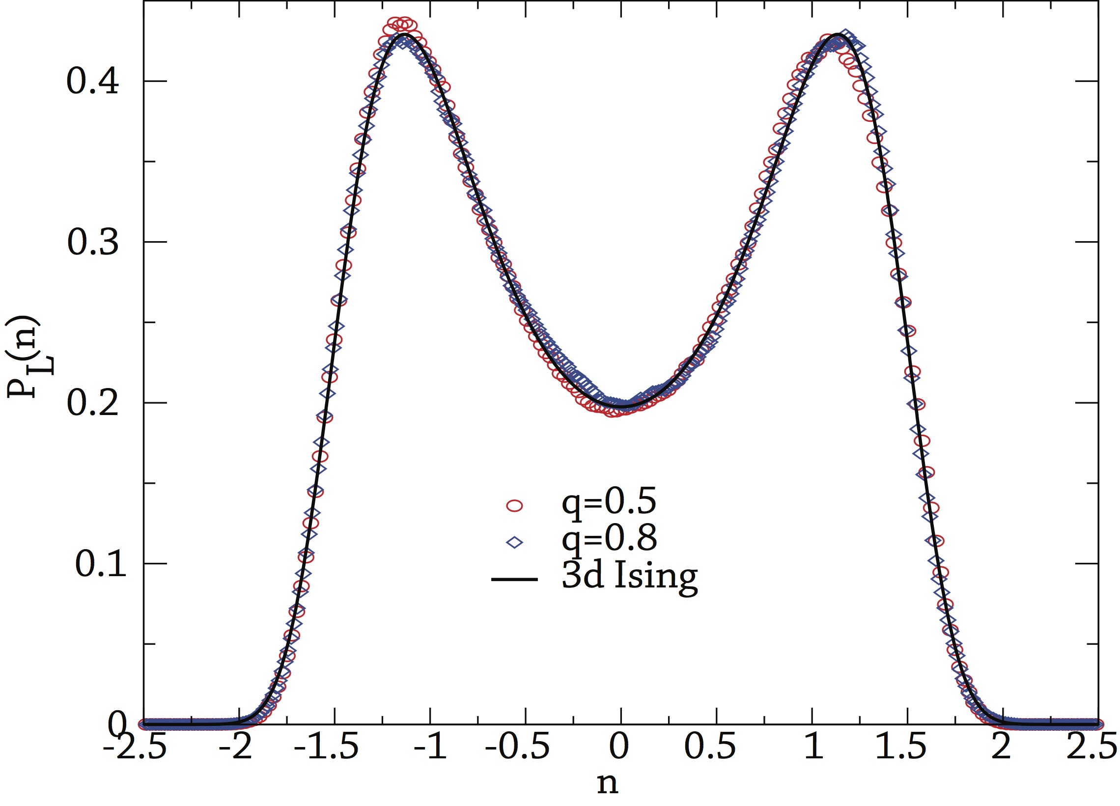
Figure 6: Critical point distribution. The abscissa is rescaled to obtain a unit variance distribution.

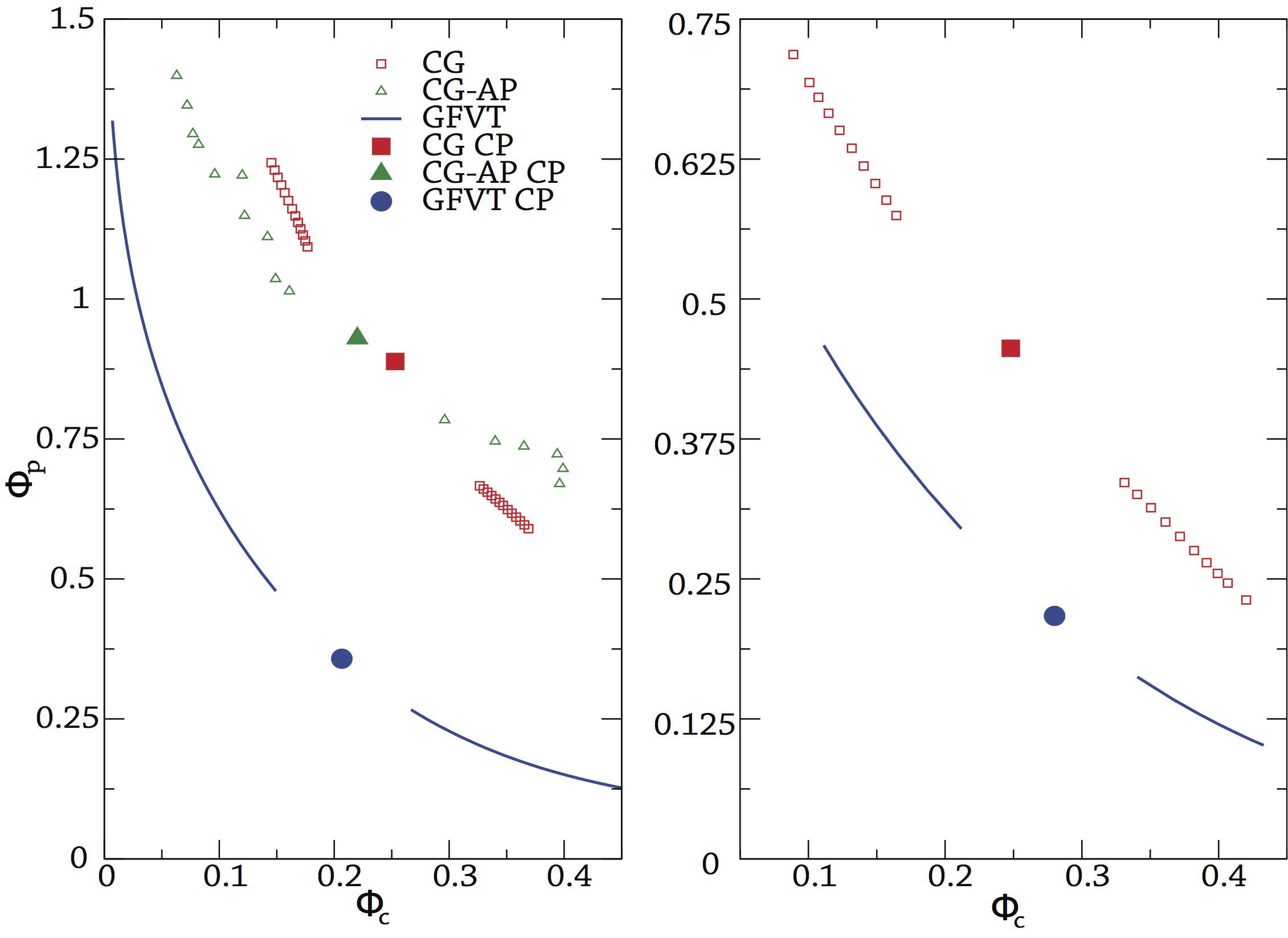
Figure 7: Fluid-fluid binodals for $q=0.8$ (left) and $q=0.5$ (right). We report the single-site (CG) result and the GFVT prediction. For $q=0.8$ we also report the binodal computed using the simplified model of Ref. AP-12 (CG-AP). For each binodal we also report the corresponding critical point (CP).

For $q=0.5$, the analysis of the data gives $z_{p,\rm crit}=2.28$ (equivalently $\Phi_{p,\rm crit}^{(r)}=0.823$), $\beta\mu_{c,\rm crit}=27.2$. Correspondingly, we have $\Phi_{c,\rm crit}=0.25$ and $\Phi_{p,\rm crit}=0.46$. We have not performed a detailed analysis of the finite-box error on these results, but it should be of the order of 0.01 on both critical volume fractions.

For $q=0.8$ the analysis of the data gives $z_{p,\rm crit}=60.11$ (equivalently $\Phi_{p,\rm crit}^{(r)}=1.621$) and $\beta\mu_{c,\rm crit}=22.9$. Correspondingly, we obtain $\Phi_{c,\rm crit}=0.25$ and $\Phi_{p,\rm crit}=0.89$.

Let us now compare the results with other estimates. For $q=0.8$ it is quite evident that the single-site binodal is located at polymer densities that are too large. This is quite evident if we consider the location of the critical point. For $q=1$ we estimated $\Phi_{c,\rm crit}=0.22$ and $\Phi_{p,\rm crit}\approx 0.62$ for the full-monomer model DPP-14-GFVT , hence the obtained estimate of $\Phi_{p,\rm crit}=0.89$ is clearly far too large. It is interesting to note that the simplified model of Ref. AP-12 gives a binodal which is not very different from the one computed here. For $q=0.5$ the single-site binodal is compatible with the upper bound provided by the full-monomer results with $q=1$. However, comparison with the GFVT results indicate that, most likely, the single-site CG model predicts phase separation at values of $\Phi_{p}$ that are too large.

Figure 8: Distribution of $\Phi_{c}$ at the binodal: (top) $q=0.8$, (bottom) $q=0.5$. We report curves for different values of $\Phi_{p}^{(r)},\beta\hat{\mu}_{c}$ (they are reported in the legend).

V Multi-site coarse-grained models

In the previous sections we have discussed single-site CG models and shown their advantages and limitations in describing the physics of the underlying microscopic system. Models with zero-density potentials are thermodynamically and structurally consistent, but are only accurate in a narrow range of densities (dilute regime) and, in the presence of colloids, for quite small polymer-to-colloid size ratios $q$. For instance, for $q=1$ we have not been able to observe phase demixing in a reasonable range of densities, while for smaller values of $q$ the polymer densities at which demixing occurs are significantly overestimated. The single-site model with state-dependent potential are only apparently more promising. They are not more accurate than those using zero-density potentials and moreover, as discussed in Sec. III, they are not thermodynamically consistent.

It seems therefore quite difficult to devise an accurate and consistent CG model at the level of the single-site representation with pairwise interactions. On the other hand, the route of single-site models with many-body, state-independent interactions is also impractical. Hence, it is tempting to abandon the single-site models in favor of the multi-site representation. For polymeric chains in the dilute and semidilute regime, multi-site representations allow us to extend the density range in which they are predictive, because of the fractal nature of the chains. The volume occupied by a long chain in solution scales like $R_{g}^{3}\sim L^{3\nu}$ where $\nu>1/3$ is the Flory scaling exponent ($\nu=0.5$ in $\theta$ solvent and $\nu\simeq 0.5876$ in good solvent). Moreover, since chains are self-similar objects, the volume occupied by each section of a chain of $\ell$ monomers (blob, $\ell\gg 1$) scales like $R_{b}^{3}(\ell)\sim\ell^{3\nu}$ where $R_{b}$ is the radius of gyration of the polymer section. We have seen that the single-site CG model with pair interactions derived at zero polymer density provides an accurate representation of polymer solutions as far as $\Phi_{p}=4\pi R_{g}^{3}N/3V$ is at most 1. Let us now divide each chain in $n$ blobs of size $\ell$ in such a way that $L=n\ell$ and let us represent each polymer section by a single interaction site. By using state-independent interactions we can expect this model to be accurate as far as $\Phi_{b}=4\pi R_{b}^{3}(\ell)nN/3V=\Phi_{p}n(\ell/L)^{3\nu}=\Phi_{p}n^{1-3\nu}\leq 1$, i.e., for $\Phi_{p}\leq n^{3\nu-1}$. Since $3\nu-1>0$, this relations implies that we can increase the density range of validity of the multi-site model and explore the semidilute regime by increasing the number of blobs per chain. Since interactions are derived at zero density these models preserve thermodynamic consistency.

These ideas were first used in constructing simple multiblob models based on pair-wise intermolecular blob interactions, simple bonding intramolecular interactions and simple transferability assumptions. In Ref. PCH-07-multi potentials obtained at zero-density were employed while in Ref. P-09-multi the potentials were optimized to reproduce properties at finite density from full monomer simulations. From these first studies it was clear that multi-site models are more difficult than their single-site analogs. The additional difficulty comes from the fact that intramolecular and intermolecular interactions have intrinsically a many-body character. When $\Phi_{p}<n^{3\nu-1}$ we can safely neglect the interactions among three or more polymer chains. However, the interactions among blobs belonging to the same molecule (intramolecular interaction) or to different molecules (intermolecular interaction) are not necessarily well represented as sums of pairwise potentials. Indeed, there is no obvious ”small” physical parameter that allows us to expand the many-body blob potentials as a sum of two-body, three-body, $\ldots$ terms. At small polymer density ($\Phi_{p}<1$), one could expect such a parameter to be the ratio between the volume of a blob and the volume of the chain $(R_{b}/R_{g})^{3}=n^{-3\nu}$. This will indeed asymptotically control the importance of two-body nonbonding interactions relative to the many-body nonbonding terms. However, this parameter does not take into account the connectivity of the chain and its topology. It should be emphasized that the nature of the CG strategy is to replace long polymers by CG models with a limited number of sites. Therefore, we would like to avoid increasing the number of blobs per chain too much, in particular, we would like to use this parameter to control the accuracy in polymer density, not the accuracy of the single-chain properties. At the same time, a good CG strategy should be able to reproduce the structural properties of a single chain (related to the intramolecular effective potential) with any number of sites in a reasonable range of $n$.

In Ref. DPP-12-Soft the first step toward such universal multi-site CG representation of polymer solutions was presented. We proposed to map a single linear chain in the scaling limit, the properties of which, suitably normalized, are universal properties of self-avoiding paths, onto a tetramer, i.e., a linear molecule with four interaction sites. The intramolecular force field of the tetramer was decomposed in two-body, three-body and four-body terms inspired by the way used in building the force fields of real molecules. Namely we introduced pair interactions between any pair of sites, three-body interactions in terms of bending angle potentials, and four-body interactions in terms of a dihedral angle potential. The potentials were obtained numerically by iteratively inverting the appropriate reduced probability densities. Details are given in Ref.DPP-12-Soft . The choice of a tetramer representation over more general $n$-mer representations with $n>4$ was dictated by simplicity reasons: the tetramer is the most elaborated representation in which all many-body interactions (up to four body) can be parametrized as scalar functions of suitably defined one-dimensional variables. In a pentamer, the coupling between the two dihedral angles requires a scalar function of two scalar variables which is more difficult to reproduce. On the other hand, we did not limit ourself to dimer or trimer representations since we could not find a suitable transferability assumption allowing us to use these models as building blocks for more refined CG models (tetramer or more blobs) while keeping the desired accuracy. The tetramer CG model was found to reproduce full monomer results for polymer solutions under good solvent conditions up to $\Phi_{p}\simeq 2$ with a $\sim 5\%$ accuracy.

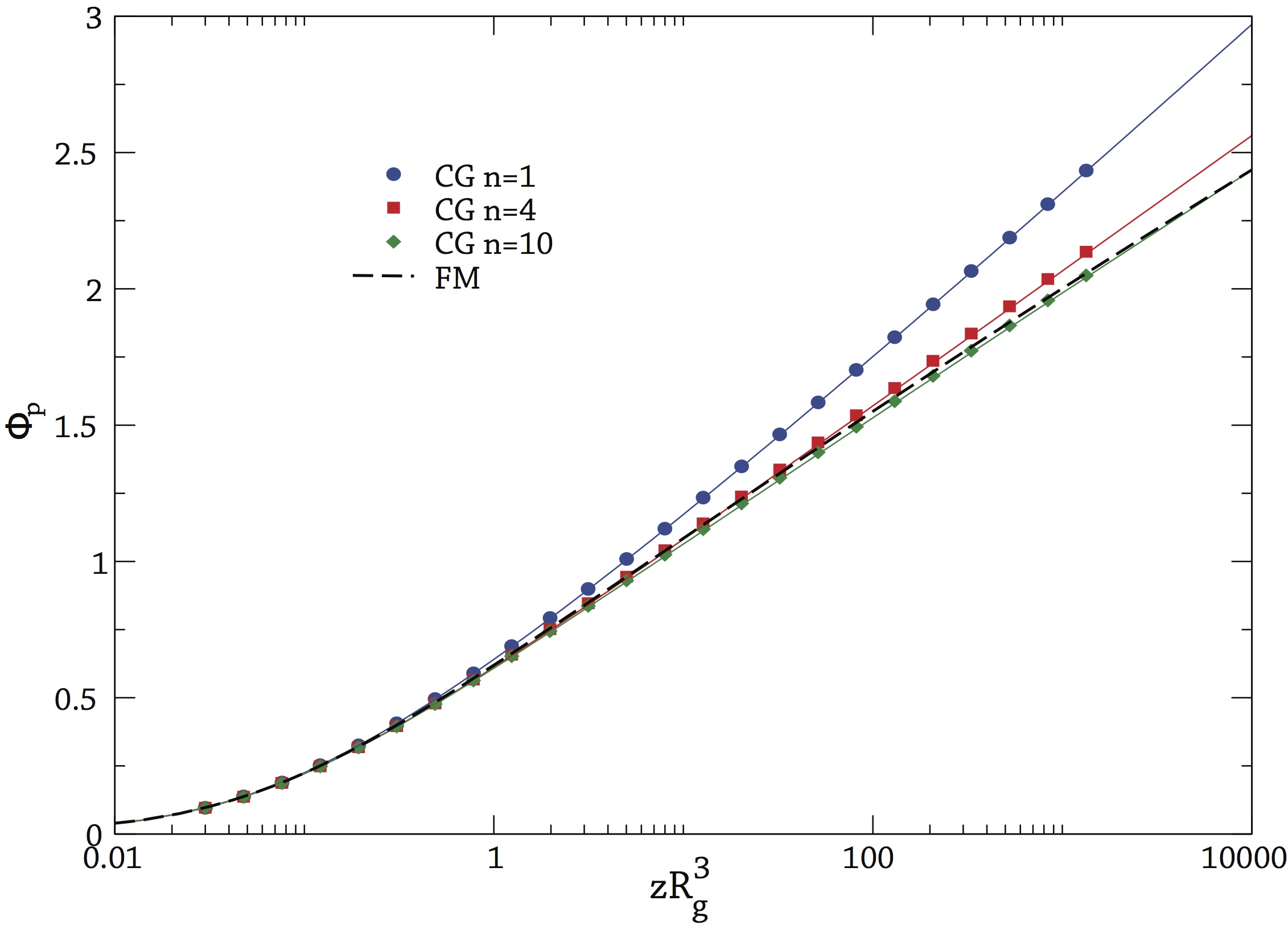
Figure 9: Grand-canonical equation of state: Polymer volume fraction $\Phi_{p}$ versus $zR^{3}_{g}$, where $z$ is the fugacity defined so that $z\approx\rho_{p}$ for small densities. We report full-monomer (FM) results, and estimates obtained by using CG models with $n=1$, 4, and 10 sites.

In a subsequent work DPP-12-MULTI , the tetramer model has been improved by an additional four-body contribution which was found to be necessary to successfully use the tetramer model as the building block for CG representations with more blobs. By employing an ad hoc transferability assumption, we have shown that this new tetramer model can be successfully used to build CG representations with more blobs per chain, which are necessary to reach larger reduced polymer densities in the semi-dilute regime. It was shown that this ”multiblob” model reproduces the leading correlation not explicitly considered in deriving the force field, namely the 5-body correlation between two subsequent dihedral angles, within $\sim$5% of accuracy, and, more importantly, that this error does not accumulate when increasing the number of blobs. The result is a consistent and transferrable CG model with variable number of interaction sites per chain that can be used to explore the thermodynamics and the structure of polymer solutions under good solvent conditions. For instance, by employing a 30-blob chains, accurate results are obtained up to $\Phi_{p}\simeq 8$. In this strategy, all potentials are derived at zero density so that standard statistical mechanics can be applied. As an example, we report in Fig. 9 the equation of state obtained by grancanonical Monte Carlo simulations. Results for the single-site model, the tetramer model, and the decamer model are compared with the universal equation of state obtained at the full-monomer level in the scaling limit. Clearly, the accuracy improves systematically by increasing the number of sites per chain.

The same strategy has been subsequently extended to the thermal crossover towards the $\theta$ point DPP-13-thermal . In this case, the temperature variable is expressed in terms of the parameter $z$ (see section 2.2). As before, we have developed the tetramer model at selected values of $z$. We have found that the tetramer model is accurate in a wider range of reduced polymer density when approaching the $\theta$ temperature. The transferability assumption to built multi-sites CG models is now more elaborated, since it must combine density and temperature, but it is equally successful, see Ref. DPP-13-thermal for details.

More recently, we have extended the tetramer model and its $n$-mer extensions to colloid-polymer mixtures in a common good solvent DPP-14-colloidi . As before we limit our intermolecular force field to pairwise central potentials. This strategy is successful only if many-body contributions to the free energy can be neglected. For this to happen we need the blob radius of gyration to be smaller than the average distance between the surface of two nearby colloids. At given reduced colloidal density $\Phi_{c}$ the average radius $R_{s}$ of the sphere containing a single colloid is $R_{s}/R_{c}=\Phi_{c}^{-1/3}$, and the average distance between the surface of two nearby colloids is $d/R_{c}=2(R_{s}-R_{c})/R_{c}=2(1-\Phi_{c}^{1/3})/\Phi_{c}^{1/3}$. Therefore, the condition is $R_{b}/R_{c}=qn^{-\nu}<2(1-\Phi_{c}^{1/3})/\Phi_{c}^{1/3}$ or, in other terms, $n>q^{1/\nu}\left[\frac{\Phi_{c}^{1/3}}{2(1-\Phi_{c}^{1/3})}\right]^{1/\nu}$ which expresses the minimum number of blobs needed for given reduce colloid density and size. Moreover, in order to treat a blob as a single site we need that $R_{b}/R_{c}<1$ (colloidal limit) which implies $n>q^{1/\nu}$. Therefore, the global condition on the suitable number of blobs is

$$n>q^{1/\nu}\max\left[1,\left(\frac{\Phi_{c}^{1/3}}{2(1-\Phi_{c}^{1/3})}\right)^{1/\nu}\right]$$ (28)

The term in square brackets is 1 for $\Phi_{c}\leq 0.3$, while is an increasing function of $\Phi_{c}$ for larger values. In ref. DPP-14-colloidi the homogenous phase of the mixture at various values of $q$ was investigated. For $q=0.5$ and $q=1$, tetramer and full-monomer are found to be in full agreement up to $\Phi_{p}=2$. For $q=2$, the tetramer slightly underestimates the depletion thickness. Nonetheless, it represents a significant improvement with respect to the single-blob model, which becomes increasingly inaccurate as $\Phi_{p}$ increases. Also the homogeneous phase of the mixture for increasing colloid density was studied DPP-14-colloidi and again the tetramer representation was found to be accurate for $q=0.5,1$ at all values of $\Phi_{p},\Phi_{c}$ in the single phase regions. At $q=2$, discrepancies between the full-monomer predictions and the tetramer results increase with increasing both $\Phi_{p}$ and $\Phi_{c}$, indicating the need of a more refined representation. By a simple transferability assumption for the blob-colloid potential we showed that the decamer representation can describe very accurately the interfacial properties of the system in the single-phase region.

VI Conclusions and outlook

In this paper we have revisited a coarse-graining strategy for polymer systems, in which a polymer chain is reduced to a single interaction site by tracing out the intramolecular degrees of freedom. The effective potential among the CG sites is inherently many-body and can be reduced to a sum of pairwise central contributions either in the low polymer-concentration limit or by allowing this effective pair-potential to depends on the thermodynamic state of the system. This CG strategy has been widely used in the past LLWAJAR-98 ; WLL-99 ; LBHM-00 ; JDLFL-01 ; BLHM-01 ; Dzubiella-etal-01 ; HG-04 ; PH-05 ; VJDL-05 ; PH-06 ; FBD-08 ; NLMC-10 ; DPP-12-compressible ; DPP-13-depletion ; DPP-14-colloidi to study polymer solutions in their homogeneous liquid phase and to address the theoretical study of the phase diagram of mixtures of non-absorbing colloids and chains of different architectures in a solvent. For homogenous polymer solutions we have shown the limits of validity of the CG single-site model with state-independent interactions (derived at zero polymer density) and discussed the apparent improvement obtained by switching to density-dependent pair interactions. The latter model is indeed tuned to represent the pair correlation function at any finite polymer concentration but it requires the knowledge of such correlation for the underlying microscopic model, a task that need to be accomplished by simulating the microscopic model itself. This fact points to a limited predictive character and weakens the relevance of this strategy. Moreover, state-dependent interactions need to be used with care as standard thermodynamic relations do not hold. Equivalent routes to physical properties for state-independent potentials provide different results when the interaction itself depends on the thermodynamic state of the system Louis-02 ; DPP-13-state-dep . We have explicitly discussed the calculation of the chain chemical potential for the homogeneous solution in Sec. III. A main consequence of this inconsistency is the failure of the equivalence among different statistical ensembles even in the thermodynamic limit DPP-13-state-dep .

These limitation were not fully recognized at first and the state-dependent CG model was used in grand-canonical simulations to study the demixing transition in colloid-polymer dispersions. This CG model exhibits a demixing transition in qualitative agreement with experiments and phenomenological theories (GFVT). As discussed in Sec. IV, we can now see that this agreement was accidental, since the phase transition in this model is driven by density fluctuations quite larger than in the underlying microscopic system. On the other hand, the CG model with zero-density interactions, which is thermodynamically consistent, is quite more accurate than the other model, but its accuracy is limited to a small range of polymer densities in the homogenous phase. Therefore, an accurate single-site CG model to describe the demixing transition of colloid-polymer dispersions seems to be out of reach.

As we have briefly reviewed in the paper, in recent years DPP-12-Soft ; DPP-12-MULTI we have developed a multi-site strategy, based on effective potentials derived at zero density, which is able to overcome these limitations and to provide thermodynamic consistent results. This new strategy is based on two main ingredients. Firstly, a suitable and transferrable representation of the intramolecular effective interaction, which allows us to keep an accurate description of single-chain properties for any number of sites per chain (level of coarse-graining of the model). Secondly, the possibility of using state-independent intermolecular interactions among CG sites of two different chains, thereby neglecting interactions among sites belonging to three or more chains, by adjusting the number of blobs per chain in such a way that the blob size be comparable to the smallest characteristic length present in the system. The strategy has been so far successfully applied to homopolymers under good-solvent conditions DPP-12-Soft ; DPP-12-MULTI and in the thermal crossover region towards the $\theta$ point DPP-13-thermal , and to colloid-polymer mixtures in the homogeneous phase DPP-14-colloidi . We are presently using this approach to compute the binodal line of the colloid-polymer mixtures at the values of $q$ for which full monomer data are absent. These results will provide the first quantitative determination of the phase diagram and will allow us to discuss on a quantitative ground the accuracy of phenomenological theories like the GFVT and the character of the experimental results (solvent quality). Note that it is also possible to incorporate in the model additional global variables, for instance the radius of gyration, as in Ref. VBK-10 (see Ref. DPP-12-compressible for the a discussion in the single-site context).

The same strategy could be applied to the most disparate situations ranging from stretched and/or confined chains, networks, brushes, polymer nanocomposites etc. The underlying principles on which our multi-site strategy is based are the fractal nature of polymers and their self-similarity. On the other hand, we expect our strategy to fail if applied to polymer melts, since the many-body character of the effective potential cannot be truncated at the lowest order by just increasing the number of sites per chain. Alternative strategies have been devised for polymer melts (see the contribution by Guenza Guenza in the same issue). However, noting that polymer-density fluctuations are much smaller in polymer melts than in solutions it might be possible that single-site CG models with state-dependent interaction provide an accurate enough description of the microscopic system and a much reduced thermodynamic inconsistency with respect to solutions. Other interesting systems for which only heuristic multi-site approaches have been used so far are di-block copolymer solutions CHC-11 , grafted polymer systems CCH-12 , and telechelic star polymer systems CCLLB-12 . It would be interesting to benchmark the predictions of such heuristic model against our systematical and controllable strategy.

VII Acknowledgments

G.D. acknowledges support from the Italian Ministry of Education Grant PRIN 2010HXAW77. Computer time has been provided by the Pisa INFN Computer Center and CINECA through the ISCRA PHCOPY HP10CFFG8Q project.

References

- (1) G. A. Voth, ed., Coarse-Graining of Condensed Phases and Biomolecular Systems (CRC Press, Boca Raton, 2009).
- (2) R. Feller, Guest Editor, Phys. Chem. Chem. Phys. 11 (2009) 1853
- (3) M. Wilson, Guest Editor, Soft Matter 5 (2009) 4341
- (4) Multiscale Modelling of Soft Matter, Faraday Discussion 144 (2010) 1
- (5) G. S. Rushbrooke and M. Silbert, Mol. Phys. 12 (1967) 505
- (6) J. S. Rowlinson, Mol. Phys. 12 (1967) 513
- (7) J. A. Barker, D. Henderson, and W. R. Smith, Mol. Phys. 17 (1969) 579
- (8) G. Casanova, R. J. Dulla, D. A. Jonah, J. S. Rowlinson, and G. Saville, Mol. Phys. 18 (1970) 589
- (9) M. A. van der Hoef and P. A. Madden, J. Chem. Phys. 111 (1999) 1520
-
(10)
C. N. Likos, Phys. Rep. 348 (2001) 267
C. N. Likos, Soft Matter 2 (2006) 478 - (11) F. Müller-Plathe, Chem. Phys. Chem. 3 (2002) 754
- (12) C. Peter and K. Kremer, Soft Matter 5 (2009) 4357
- (13) J. P. Hansen and I. McDonald, Theory of Simple Liquids, 3rd ed. (Academic Press, Amsterdam, 2006).
- (14) K. S. Schweizer and J. G. Curro, Phys. Rev. Lett. 58 (1987) 246
- (15) K. S. Schweizer and J. G. Curro, in Atomistic Modeling of Physical Properties (Springer, Berlin, 1994), p. 319.
- (16) K. S. Schweizer and J. G. Curro, Adv. Chem. Phys. 98 (1997) 1
- (17) G. D’Adamo, A. Pelissetto, and C. Pierleoni, Mol. Phys. 111 (2013) 3372
- (18) G. D’Adamo, A. Pelissetto, and C. Pierleoni, J. Chem. Phys. 141 (2014) 024902
- (19) M. Praprotnik, L. Delle Site, and K. Kremer, Ann. Rev. Phys. Chem. 59 (2008) 545
- (20) R. Potestio, S. Fritsch, P. Español, R. Delgado-Buscalioni, K. Kremer, R. Everaers, and D. Donadio, Phys. Rev. Lett. 110 (2013) 108301
- (21) P. J. Flory and W. R. Krigbaum, J. Chem. Phys. 18 (1950) 1086
- (22) A. Grosberg, P. Khalatur, and A. Khokhlov, Makromol. Chem. Rapid Commun 3 (1982) 709
- (23) A. B. Krüger and L. Schäfer, J. Physique 50 (1989) 3191
- (24) J. Dautenhahn and C. Hall, Macromolecules 27 (1994) 5399
- (25) C. N. Likos, H. Löwen, M. Watzlawek, B. Abbas, O. Jucknischke, J. Allgaier, and D. Richter, Phys. Rev. Lett. 80 (1998) 4450
- (26) M. Watzlawek, C. N. Likos, and H. Löwen, Phys. Rev. Lett. 82 (1999) 5289
- (27) A. A. Louis, P. G. Bolhuis, J. P. Hansen, and E. J. Meijer, Phys. Rev. Lett. 85 (2000) 2522
- (28) A. Jusufi, J. Dzubiella, C. N. Likos, C. von Ferber, and H. Löwen, J. Phys.: Condens. Matter 13 (2001) 6177
- (29) P. G. Bolhuis, A. A. Louis, J. P. Hansen, and E. J. Meijer, J. Chem. Phys. 114 (2001) 4296
- (30) S. Asakura and F. Oosawa, J. Chem. Phys. 22 (1954) 1255
- (31) P. G. Bolhuis, A. A. Louis, and J. P. Hansen, Phys. Rev. E 64 (2001) 021801
- (32) A. Pelissetto and J.-P. Hansen, J. Chem. Phys. 122 (2005) 134904
- (33) G. D’Adamo, A. Pelissetto, and C. Pierleoni, Soft Matter 8 (2012) 5151
- (34) G. D’Adamo, A. Pelissetto, and C. Pierleoni, J. Chem. Phys. 136 (2012) 224905
- (35) D. Reith, M. Pütz, and F. Müller-Plathe, J. Comput. Chem. 24 (2003) 1624
- (36) A. Lyubartsev and A. Laaksonen, Phys. Rev. E 52 (1995) 3730
- (37) A. Soper, Chem. Phys. 202 (1996) 295
- (38) P. G. Bolhuis and A. A. Louis, Macromolecules 35 (2002) 1860
- (39) G. D’Adamo, A. Pelissetto, and C. Pierleoni, J. Chem. Phys. 138 (2013) 234107
- (40) A. A. Louis, J. Phys.: Condens. Matter 14 (2002) 9187
- (41) J. Dzubiella, C. N. Likos, and H. Löwen, J. Chem. Phys. 116 (2002) 9518
- (42) R. Menichetti and A. Pelissetto, J. Chem. Phys. 138 (2013) 124902
- (43) L. Liu, W. K. Den Otter, and W. J Briels, Soft Matter 39 (2014) 7874
- (44) G. D’Adamo, A. Pelissetto, and C. Pierleoni, J. Chem. Phys. 139 (2013) 034901
- (45) A. Vrij, Pure and Appl. Chem. 48 (1976) 471
- (46) T. A. Witten and P. A. Pincus, Macromolecules 19 (1986) 2509
- (47) H.-P. Hsu and P. Grassberger, Europhys. Lett. 66 (2004) 874
- (48) A. Pelissetto, Phys. Rev. E 85 (2012) 021803
- (49) P. Attard, Thermodynamics and Statistical Mechanics: Equilibrium by Entropy Maximisation (Academic Press, Waltham, Massachusetts, 2002).
- (50) D. J. Ashton and N. B. Wilding, J. Chem. Phys. 140 (2014) 244118
- (51) P. G. de Gennes, Scaling Concepts in Polymer Physics (Cornell University Press, Ithaca, NY, 1979).
- (52) J. des Cloizeaux and G. Jannink, Polymers in Solution: Their Modelling and Structure (Clarendon, Oxford, 1990).
- (53) L. Schäfer, Excluded Volume Effects in Polymer Solutions (Springer Verlag, Berlin, 1999).
- (54) C. Domb and G. S. Joyce, J. Phys. C 5 (1972) 956
- (55) S. Caracciolo, B. M. Mognetti, and A. Pelissetto, J. Chem. Phys. 125 (2006) 094903
- (56) A. Pelissetto, J. Chem. Phys. 129 (2008) 044901
- (57) F. Randisi and A. Pelissetto, J. Chem. Phys. 139 (2013) 154902.
- (58) N. Madras and A. D. Sokal, J. Stat. Phys. 50 (1988) 109
- (59) T. Kennedy, J. Stat. Phys. 106 (2002) 407
- (60) N. Clisby, J. Stat. Phys. 140 (2010) 349
- (61) C. von Ferber, A. Jusufi, M. Watzlawek, C. N. Likos, and H. Löwen, Phys. Rev. E 62 (2000) 6949
- (62) B. H. Zimm, W. H. Stockmayer, and M. Fixman, J. Chem. Phys. 21 (1953) 1716
- (63) S. Caracciolo, B. M. Mognetti, and A. Pelissetto, J. Chem. Phys. 128 (2008) 065104
- (64) G. C. Berry, J. Chem. Phys. 44 (1966) 4550
- (65) T. Norisuye, K. Kawahara, A. Teramoto, and H. Fujita, J. Chem. Phys 49 (1968) 4330
- (66) T. Matsumoto, N. Nishioka, and H. Fujita, J. Polym. Sci.: Part A-2 Polym. Phys. 10 (1972) 23
- (67) Y. Nakamura, T. Norisuye, and A. Teramoto, Macromolecules 24 (1991) 4904
- (68) K. Akasaka, Y. Nakamura, T. Norisuye, and A. Teramoto, Polym. J. 26 (1994) 363
- (69) V. Krakoviack, J. P. Hansen, and A. A. Louis, Phys. Rev. E 67 (2003) 041801
- (70) C. I. Addison, A. A. Louis, and J. P. Hansen, J. Chem. Phys. 121 (2004) 9612
- (71) F. H. Stillinger, H. Sakai, and S. Torquato, J. Chem. Phys. 117 (2002) 288
- (72) M. E. Johnson, T. Head-Gordon, and A. A. Louis, J. Chem. Phys. 126 (2007) 144509
- (73) L. Henderson, Phys. Lett. 49A (1974) 197
- (74) J. T. Chayes, L. Chayes, and E. H. Lieb, Comm. Math. Phys. 93 (1984) 57
- (75) T. Morita, Prog. Theor. Phys. 23 (1960) 829
- (76) P. Attard, J. Chem. Phys. 94 (1991) 2370
- (77) B. Widom, J. Chem. Phys. 39 (1963) 2802
- (78) A. Fortini, P. G. Bolhuis, and M Dijkstra, J. Chem. Phys. 128 (2008) 024904
- (79) W. C. K. Poon, J. Phys.: Condensed Matter 14 (2002) R859
- (80) M. Fuchs and K. S. Schweizer, J. Phys.: Condensed Matter 14 (2002) R239
- (81) R. Tuinier, J. Rieger, and C. G. de Kruif, Adv. Colloid Interface Sci. 103 (2003) 1
- (82) K. J. Mutch, J. S. van Duijneveldt, and J. Eastoe, Soft Matter 3 (2007) 155
- (83) G. J. Fleer and R. Tuinier, Adv. Coll. Interface Sci. 143 (2008) 1
- (84) O. Myakonkaya and J. Eastoe, Adv. Coll. Interface Sci. 149 (2009) 39
- (85) P. G. Bolhuis, A. A. Louis, and J. P. Hansen, Phys. Rev. Lett. 89 (2002) 128302
- (86) J. Dzubiella, A. Jusufi, C. N. Likos, C. von Ferber, H. Löwen, J. Stellbrink, J. Allgaier, D. Richter, A. B. Schofield, P. A. Smith, W. C. K. Poon, and P. N. Pusey, Phys. Rev. E 64 (2001) 010401(R)
- (87) M. Schmidt, A. R. Denton, and J. M. Brader, J. Chem. Phys. 118 (2003) 1541
- (88) R. L. C. Vink, A. Jusufi, J. Dzubiella, and C. N. Likos, Phys. Rev. E 72s (2005) 030401(R)
- (89) A. Pelissetto and J. P. Hansen, Macromolecules 39 (2006) 9571
-
(90)
J. Zausch, P. Virnau, K. Binder, J. Horbach, R. L. C. Vink,
J. Chem. Phys. 130 (2009) 064906
J. Zausch, J. Horbach, P. Virnau, and K. Binder, J. Phys.: Condens. Matter 22 (2010) 104120 - (91) M. A. Annunziata and A. Pelissetto, Phys. Rev. E 86 (2012) 041804
- (92) G. D’Adamo, A. Pelissetto, and C. Pierleoni, J. Chem. Phys. 141 (2014) 244905.
- (93) C.-Y. Chou, T. T. M. Vo, A. Z. Panagiotopoulos, and M. Robert, Physica A 369 (2006) 275
- (94) N. A. Mahynski, T. Lafitte, and A. Z. Panagiotopoulos, Phys. Rev. E 85 (2012) 051402
- (95) N. A. Mahynski, B. Irick, and A. Z. Panagiotopoulos, Phys. Rev. E 87 (2013) 022309
- (96) D. G. L. Aarts, R. Tuinier, and H. N. W. Lekkerkerker, J. Phys.: Condens. Matt. 14 (2002) 7551.
- (97) G. J. Fleer and R. Tuinier, Phys. Rev. E 76 (2007) 041802
- (98) R. Tuinier, P. A. Smith, W. C. K. Poon, S. U. Egelhaaf, D. G. A. L. Aarts, H. N. W. Lekkerkerker, and G. J. Fleer, Europhys. Lett. 82 (2008) 68002
- (99) H. N. W. Lekkerkerker and R. Tuinier, Colloids and the Depletion Interaction, Lect. Notes Phys. 833 (Springer, Berlin, 2011)
- (100) G. M. Torrie and J. P. Valleau, J. Comp. Phys. 23 (1977) 197
- (101) A. Pelissetto and F. Ricci-Tersenghi, in Large Deviations in Physics: The Legacy of the Law of Large Numbers, edited by A. Vulpiani, F. Cecconi, M. Cencini, A. Puglisi, and D. Vergni, Lect. Notes Phys. 885 (2014) 161.
- (102) R. L. C. Vink and J. Horbach, J. Chem. Phys. 121 (2004) 3253
- (103) R. L. C. Vink, in Computer Simulation Studies in Condensed Matter Physics XVIII, edited by D. P. Landau, S. P. Lewis, and H. B. Schuettler (Springer, Berlin, 2004).
- (104) A. M. Ferrenberg and R. H. Swendsen, Phys. Rev. Lett. 63 (1989) 1195
- (105) N. B. Wilding, J. Phys.: Condens. Matter 9 (1997) 585
- (106) M. M. Tsypin and H. W. J. Blöte, Phys. Rev. E 62 (2000) 73
- (107) C. Pierleoni, B. Capone and J. P. Hansen, J. Chem. Phys. 127 (2007) 171102
- (108) A. Pelissetto, J. Phys.: Condens. Matter 21 (2009) 115108
- (109) G. D’Adamo, A. Pelissetto, and C. Pierleoni, J. Chem. Phys. 137 (2012) 024901
- (110) A. Narros, C. N. Likos, A. J. Moreno, and B. Capone, Soft matter 10 (2010) 9601
- (111) T. Vettorel, G. Besold, and K. Kremer, Soft Matter 6 (2010) 2282
-
(112)
M. G. Guenza, this volume.
A. J. Clark and M. G. Guenza, J. Chem. Phys. 132 (2010) 044902 - (113) B. Capone, J.P. Hansen, and I. Coluzza, J. Phys. Cond. Matter 23 (2011) 194102
- (114) I. Coluzza, B. Capone, and J.-P. Hansen, Soft Matter 7 (2011) 5255
- (115) B. Capone, I. Coluzza, F. G. Lo Verso, C. N. Likos, and R. Blaak, Phys. Rev. Lett. 109 (2012) 238301