Jet-ISM Interaction in the Radio Galaxy 3C 293: Jet-driven Shocks Heat ISM to Power X-ray and Molecular H₂ Emission

Abstract

We present a 70 ks Chandra observation of the radio galaxy 3C 293. This galaxy belongs to the class of molecular hydrogen emission galaxies (MOHEGs) that have very luminous emission from warm molecular hydrogen. In radio galaxies, the molecular gas appears to be heated by jet-driven shocks, but exactly how this mechanism works is still poorly understood. With Chandra, we observe X-ray emission from the jets within the host galaxy and along the 100 kpc radio jets. We model the X-ray spectra of the nucleus, the inner jets, and the X-ray features along the extended radio jets. Both the nucleus and the inner jets show evidence of $10^{7}$ K shock-heated gas. The kinetic power of the jets is more than sufficient to heat the X-ray emitting gas within the host galaxy. The thermal X-ray and warm H₂ luminosities of 3C 293 are similar, indicating similar masses of X-ray hot gas and warm molecular gas. This is consistent with a picture where both derive from a multiphase, shocked interstellar medium (ISM). We find that radio-loud MOHEGs that are not brightest cluster galaxies (BCGs), like 3C 293, typically have $L_{H_{2}}/L_{X}\sim 1$ and $M_{H_{2}}/M_{X}\sim 1$, whereas MOHEGs that are BCGs have $L_{H_{2}}/L_{X}\sim 0.01$ and $M_{H_{2}}/M_{X}\sim 0.01$. The more massive, virialized, hot atmosphere in BCGs overwhelms any direct X-ray emission from current jet-ISM interaction. On the other hand, $L_{H_{2}}/L_{X}\sim 1$ in the Spiderweb BCG at z=2, which resides in an unvirialized protocluster and hosts a powerful radio source. Over time, jet-ISM interaction may contribute to the establishment of a hot atmosphere in BCGs and other massive elliptical galaxies.

1. INTRODUCTION

1.1. AGN Feedback via Radio Jets

Feedback from active galactic nuclei (AGN) is thought to play an important role in the evolution of galaxies. In numerical simulations, it has been shown to clear galaxies of gas and suppress star formation and supermassive black hole growth (e.g., Silk & Rees, 1998; Di Matteo et al., 2005). One type of feedback may take the form of interactions between radio jets and the interstellar medium (ISM), which may have either positive or negative effects on the star formation rate (Wagner & Bicknell, 2011). Hydrodynamical simulations of such interactions show that radio jets can create cocoons of hot X-ray emitting gas by depositing energy into the galaxy’s ISM, which in turn can spread the effect of the jets to the entire host galaxy as the bubbles expand (Sutherland & Bicknell, 2007). In effect, radio jets can suppress star formation by driving shocks and turbulence into the ISM, thereby making the molecular gas inhospitable to forming stars, or by driving outflows that strip the galaxy of the raw materials from which stars form (e.g., Guillard et al., 2012). Neutral and ionized outflows are observed in radio galaxies (e.g., Morganti et al., 2003, 2005; Emonts et al., 2005; Mahony et al., 2013; Holt et al., 2008; Lehnert et al., 2011; Crenshaw et al., 2003; Morganti et al., 2013) with velocities that can exceed 1000 km s^-1 and mass outflow rates of up to 60 M_⊙ yr^-1 for the neutral component. Additionally, a growing number of jet-driven outflows of both cold and warm molecular gas have been found recently (e.g., Dasyra & Combes, 2012; Dasyra et al., 2014; Combes et al., 2013; Morganti et al., 2013; García-Burillo et al., 2014; Fischer et al., 2010; Sturm et al., 2011).

Table 1X-ray Sources

Name	Label	RA(J2000)	Dec(J2000)	Aperture
UGC 08782	Nucleus$+$Host	13h 52m 17.81s	+31d 26m 46.1s	$3\farcs 5$ circle; 20′′ circle
CXO J135217.8 +312646	NC	13h 52m 17.79s	+31d 26m 46.6s	$1\farcs 0\times 1\farcs 4$ ellipse with PA=90∘
CXOU J135217.9 +312646	NE0	13h 52m 17.91s	+31d 26m 46.4s	$0.8^{\prime\prime}$ circle
CXOU J135212.9 +312737	NW1	13h 52m 12.9s	+31d 27m 37.0s	$6^{\prime\prime}$ circle
CXOU J135212.0 +312754	NW2	13h 52m 12.0s	+31d 27m 54.1s	$12\farcs 9\times 8\farcs 7$ ellipse with PA=30∘
CXOU J135221.5 +312621	SE1	13h 52m 21.5s	+31d 26m 21.0s	polygon
CXOU J135224.9 +312510	SE2	13h 52m 24.9s	+31d 25m 10.0s	$13\farcs 2\times 8\farcs 0$ ellipse with PA=300∘
CXOU J135214.4 +312717	NPS	13h 52m 14.4s	+31d 27m 17.5s	$3^{\prime\prime}$ circle
CXOU J135225.2 +312537	SPS	13h 52m 25.2s	+31d 25m 37.3s	$4^{\prime\prime}$ circle
CXOU J135218.9 +312647	EPS	13h 52m 18.9s	+31d 26m 47.6s	$2^{\prime\prime}$ circle

1.2. Molecular Hydrogen Emission Galaxies

A new class of galaxies with extremely luminous, high equivalent width H₂ emission lines in the infrared (IR) was discovered using the Spitzer Space Telescope (Werner et al., 2004), now referred to as molecular hydrogen emission galaxies (MOHEGs). Examples include the radio galaxy 3C 326 (Ogle et al., 2007), the brightest cluster galaxy in Zw 3146 (Egami et al., 2006), Stephan’s Quintet (NGC 7318b; Appleton et al., 2006), and the Taffy bridge (Peterson et al., 2012). Spitzer IRS observations of such galaxies find mid-IR H₂ luminosities of $L(H_{2})=10^{38}-10^{45}$ erg s^-1, and H₂ to IR luminosity ratios of $L_{H_{2}}/L_{8-1000\,\mu{\rm m}}=0.001-0.1$. The MOHEG class (Ogle et al., 2010) is defined to have L(H₂ 0-0 S(0)$-$S(3))/L(PAH 7.7 $\mu$m)$>0.04$, a ratio that is too large to be produced by photodissociation regions in star-forming regions (Guillard et al., 2012).

The molecular hydrogen responsible for this emission may be heated by three potential mechanisms. The first is X-ray heating by active galactic nuclei (AGNs) or other X-ray sources. However, Ogle et al. (2010) showed that radio MOHEGs do not contain the high-luminosity, high-ionization AGN necessary to produce the observed H₂ emission. The second mechanism of cosmic ray heating cannot be ruled out but requires a very high cosmic ray density (Ogle et al., 2010). The third mechanism of shock heating, previously seen in radio galaxies (e.g., Labiano et al., 2013; Guillard et al., 2012; Scharwächter et al., 2013), is therefore deemed most likely. These shocks may be propagated due to the interaction of the radio jet and the ISM of the host galaxy.

1.3. 3C 293

3C 293 is one of brightest H₂ emitters of a sample of 55 radio galaxies observed by Spitzer (Ogle et al., 2010), which were selected by redshift ($z<0.22$) and radio flux. 3C 293 was one of the 17/55 of these galaxies to fall into the MOHEG regime with L(H₂ 0-0 S(0)$-$S(3))/L(PAH 7.7 $\mu$m)=0.24. Its host galaxy is highly irregular and appears to be interacting with a less massive companion to the southwest. A tidal bridge connects the two galaxies, similar to the 3C 326 system. The large scale radio morphology 3C 293 is intermediate between Fanaroff and Riley (FR; 1974) I and FR II. Its radio luminosity $\nu L_{\nu}{\rm(178\,MHz)}=1.1\times 10^{41}\,{\rm erg\,s^{-1}}$ is characteristic of an FR I, but it has the hot-spot morphology of an FR II. The bright radio core is resolved by Multi-Element Radio Linked Interferometric Network (MERLIN), revealing a double-lobed compact-symmetric source, which appears to bend out of the galactic disk. (Akujor et al., 1996; Beswick et al., 2002, 2004). CO observations of this galaxy indicate a large cold H₂ mass of $2.2\times 10^{10}$ M_⊙ (Evans et al., 1999; Labiano et al., 2013). Additionally, strong outflows have been detected: Morganti et al. (2003) and Mahony et al. (2013) detected a neutral H i outflow up to 1000 km s^-1 containing $\sim 10^{7}\,M_{\odot}$, and Emonts et al. (2005) detected a ionized outflow with $\sim 10^{5}\,M_{\odot}$.

In this paper, we present a Chandra observation of 3C 293 and study the impact of jet feedback in this galaxy. Section 2 presents the observations and data reduction. We describe the X-ray morphology in Section 3 and present the X-ray spectra of various components in Section 4. In Section 5, we discuss the effect of the jet on the interstellar medium of 3C 293 and the peculiar X-ray features observed along the large scale jets. Distance-dependent quantities in this paper are calculated using cosmological parameters $H_{0}=70\,{\rm km\,s^{-1}\,Mpc^{-1}}$, $\Omega_{M}=0.3$, and $\Omega_{\Lambda}=0.7$. With a redshift of 0.045 (de Vaucouleurs et al., 1991), these assumptions yield a distance of 199.3 Mpc for 3C 293 at which 1^′′ corresponds to 0.97 kpc.

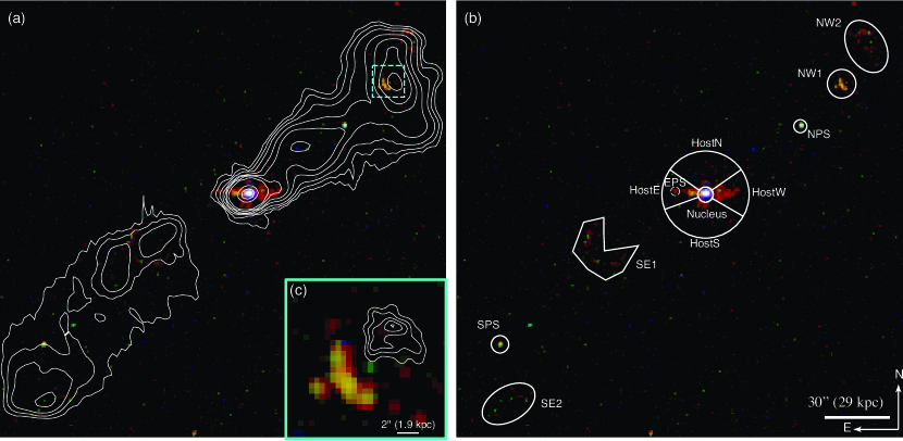
Figure 1.— Chandra image of 3C 293 showing soft (0.5$-$1.5 keV) emission in red, medium (1.5$-$3.0 keV) in green, and hard (3.0$-$8.0 keV) in blue, overlaid with the 1.4 GHz contours (a; contours levels at 0.0005, 0.001, 0.002, 0.005, 0.01, 0.02, 0.05, 1.0, and 2.0 Jy/beam) and spectral extraction apertures (b). Two jets emerge from the nucleus in the East-West direction, dominated by soft emission. Several extended features are present along the extended jets, primarily in the soft and medium bands, as well as two point sources. SE1 lies in a region of diminished radio emission compared to the jet on either side of it. NW2 and SE2 exist on the edge of the radio jets. Panel (c) shows contours of a higher resolution 1.4 GHz image (3.25, 4.5, 5.75, 7, and 8.25 mJy/beam) showing the location of the NW radio hotspot relative to NW1.

2. OBSERVATIONS AND DATA REDUCTION

2.1. X-ray Spectra

3C 293 was observed for 67.8 ks on 2010 November 16 (ObsID 12712, PI P. Ogle) with the back-illuminated CCD chip, S3, of the Chandra Advanced CCD Imaging Spectrometer (ACIS; Weisskopf et al., 2000) in faint data mode. We reprocessed the observation using ciao version 4.5 to create a new level 2 events file, following the software threads from the Chandra X-ray Center (CXC). We measured the counts in each aperture shown in Figures 1b and 2 and listed in Table 1. X-ray spectra were extracted using the specextract task in the 0.3$-$8.0 keV energy range from ten regions of interest with at least $\sim$100 net counts. We grouped the data for each region to have a minimum of 10 counts per bin and compared the results to the background emission, measured in large source-less regions on the same chip, to determine the energy range over which the source had significant counts. We filtered the data based on that energy range and then grouped it to a minimum of 20 counts per bin prior to modeling the spectra (as described in Section 4). Counts and the luminosities derived from fitting these spectra are listed in Table 2.

2.2. Spitzer Imaging

We retrieved Infrared Array Camera (IRAC; Fazio et al., 2004) observations of 3C 293 taken by the Spitzer Space Telescope (Werner et al., 2004) on 2005 June 11 (PID 3418, PI M. Birkinshaw) at 3.6 $\mu$m, 4.5 $\mu$m, 5.8 $\mu$m, and 8.0 $\mu$m consisting of 24$\times$30 s frames, covering the galaxy and the nearby field. The Multiband Imaging Photometer (MIPS; Rieke et al., 2004) observations were also obtained from the Spitzer Heritage Archive. MIPS observed 3C 293 in the 24 $\mu$m band on 2005 June 28 (PID 82, PI G. Rieke; 56$\times$2.62 s frames), 2007 July 19 (PID 40053, PI G. Rieke; 56$\times$2.62 s frames), and 2009 February 9 (PID 50099; 28$\times$2.62 s frames). As part of the 2005 observation, MIPS also imaged 3C 293 at 70 $\mu$m (28$\times$10.49 s frames) and 160 $\mu$m (68$\times$10.49 s frames). Mosaics were created using Mosaicker and Point source Extractor package (MOPEX; Makovoz & Khan, 2005) for all seven bands with $0\farcs 6$ pixels in the IRAC bands and $2\farcs 45$ pixels in the MIPS bands.

2.3. Spitzer Spectral Imaging

3C 293 was observed with the Infrared Spectrograph (IRS; Houck et al., 2004) on Spitzer in the mapping mode in the SL1,2 and LL1,2 modules (PID 20719, PI S. Baum; 2006 January 18). The 14 s observations were stepped perpendicular to the slit in each module. Spectral cubes were constructed for each module using the IDL program cubism (Smith et al., 2007), using the off-pointed slit for background subtraction and removing global bad pixels. We extracted slices of the spectral cubes at the wavelengths of the rotational H₂ lines (i.e., 17.03 $\mu$m 0-0 S(1), 9.66 $\mu$m 0-0 S(3), 6.91 $\mu$m 0-0 S(5), and 5.55 $\mu$m 0-0 S(7)). IRS also observed 3C 293 in staring mode on 2007 June 19 (PID 30877, PI A. Evans; previously published in Guillard et al., 2012). We measured the spatial extent of the H₂ lines and the [NeII] line.

2.4. Ancillary Imaging

Ancillary images were collected from the archives of the Galaxy Evolution Explorer (GALEX in far-UV and near-UV; Martin et al., 2005), Sloan Digital Sky Survey (SDSS DR10 in ugriz; Ahn et al., 2014) and Two Micron All Sky Survey (2MASS in J, H, and Ks; Skrutskie et al., 2006). We extracted photometry in a common 30^′′ aperture centered on the X-ray nucleus in each band, as well as in the Spitzer images described above. We also retrieved Infrared Astronomical Satellite (IRAS) photometry (Golombek et al., 1988) from the NASA Extragalactic Database (NED).

We observed 3C 293 with the 2.4 m Hiltner telescope of the Michigan-Dartmouth-MIT (MDM) observatory on 2007 March 14 in the B filter. Observations were done by integrating 60 min at an airmass of $1.0-1.1$ under seeing conditions of $\sim$1.2 arcsec. The observations and data reduction were performed in the same way as those described in Emonts et al. (2010).

We used archival observations taken by the Very Large Array (VLA) to make images of the source at 1.4 GHz and 8.4 GHz. The 1.4 GHz image of the large scale radio jets was taken on 1999 November 18 in L band in B configuration for 1.3 hrs (PID GP022, Beswick et al., 2004). The 8.4 GHz image of the core region was observed on 1995 July 27 in X band in A configuration for 0.11 hrs (PID AK403). We also used a 1.4 GHz VLA image taken in A configuration on 2000 November 25 (PID AM670, PI R. Morganti), whose observation and data reduction were described in Emonts (2006) and which shows the structure of the northwest hotspot in greater detail.

Table 2X-ray Counts and Luminosities

Region	Net Counts	Hardness	Flux (10-14 erg cm-2 s-1)	Lumin. (1040 erg s-1)
	0.4$-$8.0 keV	Ratio	0.4$-$8.0 keV	0.4$-$8.0 keV
Nucleus	2130$\pm$50	0.75${}^{+0.01}_{-0.02}$	$76.6^{+~{}\,6.9}_{-13.4}$	$364^{+33}_{-64}$
NC	1810$\pm$40	0.87${}^{+0.01}_{-0.01}$	$87.6^{+~{}\,5.2}_{-11.8}$	$416^{+25}_{-56}$
NE0	194$\pm$14	0.17${}^{+0.07}_{-0.07}$	$7.22^{+1.46}_{-1.24}$	$34.3^{+6.9}_{-5.9}$
Host: East	160$\pm$14	-0.75${}^{+0.07}_{-0.07}$	$1.38^{+0.61}_{-0.29}$	$6.54^{+2.89}_{-1.37}$
Host: West	184$\pm$15	-0.81${}^{+0.07}_{-0.06}$	$1.08^{+0.12}_{-0.15}$	$5.15^{+0.58}_{-0.69}$
Host: North	87$\pm$12	-0.32${}^{+0.13}_{-0.16}$	$0.59^{+0.24}_{-0.15}$	$2.81^{+1.13}_{-0.69}$
Host: South	99$\pm$13	-0.32${}^{+0.15}_{-0.13}$	$0.78^{+0.24}_{-0.17}$	$3.73^{+1.13}_{-0.74}$
NW1	119$\pm$12	-0.58${}^{+0.09}_{-0.09}$	$1.20^{+0.28}_{-0.25}$	$5.70^{+1.34}_{-1.18}$
NW2	98$\pm$12	-0.68${}^{+0.15}_{-0.14}$	$0.87^{+0.19}_{-0.15}$	$4.16^{+0.88}_{-0.71}$
SE1	109$\pm$13	-0.63${}^{+0.16}_{-0.12}$	$1.15^{+0.40}_{-0.23}$	$5.49^{+1.91}_{-1.07}$
SE2	47$\pm$10	-0.76${}^{+0.07}_{-0.24}$	$0.71^{+0.16}_{-0.15}$	$3.37^{+0.76}_{-0.73}$
NPS	68$\pm$  8	-0.08${}^{+0.13}_{-0.12}$	$1.42^{+0.28}_{-0.30}$	$6.75^{+1.34}_{-1.43}$
SPS	43$\pm$  7	-0.41${}^{+0.15}_{-0.17}$	$0.56^{+0.11}_{-0.11}$	$2.67^{+0.53}_{-0.52}$
EPS	13$\pm$  4	-0.9	…	…

3. X-ray Morphology

Figure 1b shows a three-color (soft, medium, and hard) X-ray image taken by Chandra overlaid with the apertures on interesting features from which we extract integrated counts (see Table 2) and spectra. These features fall into four types: central region (nucleus), extended emission in the host galaxy (hostN, hostS, hostE, and hostW), large scale jet-related features (NW1, NW2, SE1, and SE2), and point sources (SPS, NPS, and EPS) along the jets. Figures 1a, 1c, and 2 show the relation of the X-ray and radio emission.

3.1. Nuclear Region

3C 293 has a strong X-ray core (detected with $\sim 2100$ counts). Figure 2 shows the nuclear region in detail with the X-ray data binned into 0$\farcs$25 pixels. High resolution radio observations (e.g., Beswick et al., 2002, 2004; Akujor et al., 1996) show a small scale radio (8.4 GHz) jet. To the east of the nucleus, there is a softer X-ray feature coincident with a knot of radio emission, which is also the launch site of the ionized outflow (Emonts et al., 2005). The radio jet appears to bend $30^{\circ}$ to the southeast after about 1.7 kpc, continuing for another $1.5$ kpc. In contrast, the western jet does not show a bend, is only $1.4$ kpc, and does not have a similar X-ray counterpart. The neutral outflow is associated with this western jet (Mahony et al., 2013). Observations of the radio jet by Akujor et al. (1996) detected faint diffuse emission out to $\sim 4$ kpc, which they suggest could belong to an outburst older than the one responsible for the $<2$ kpc jets.

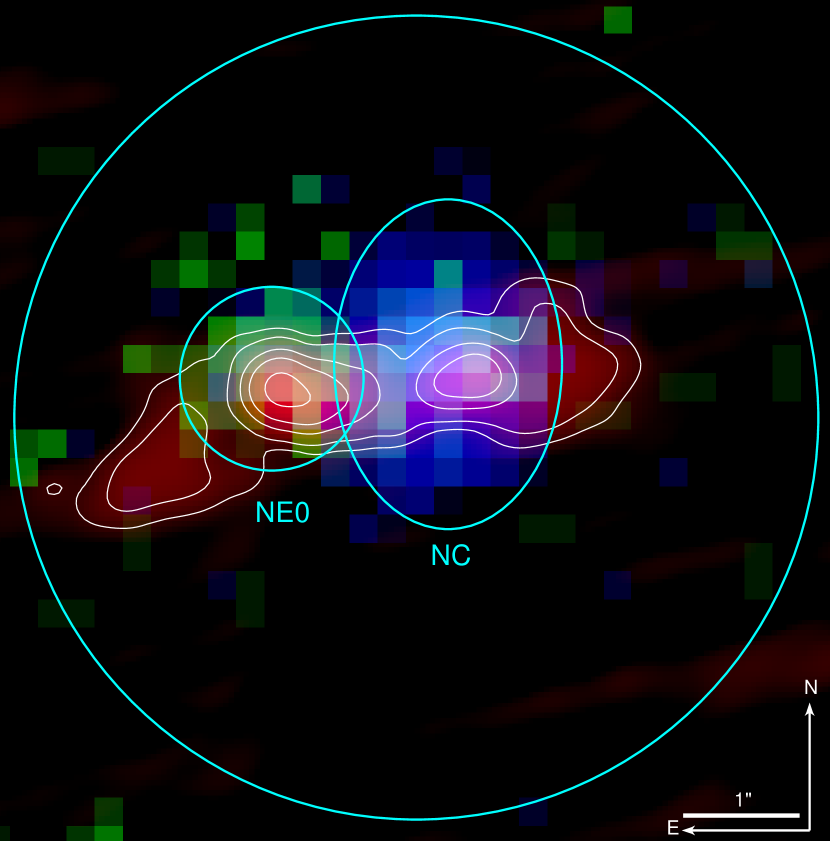
Figure 2.— Chandra (green: 0.5$-$1.5 keV; blue: 1.5$-$8.0 keV) and VLA (red and white contours: 8.4 GHz) image of the nuclear region overlaid with the nuclear extraction aperture. To the east of the hard X-ray point source (NC) there is a softer component (NE0), which is approximately coincident with a knot in the very small radio jet, in turn the expected launch site of the ionized outflow.

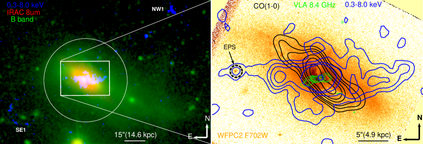
Figure 3.— Multiwavelength image showing that the X-ray emission (blue) extends through most of the host galaxy’s optical emission (green; B-band) and past the bulk of the MIR (red; IRAC 8.0 $\mu$m). The features along the large jets (e.g., NW1 and SE1) are beyond the host galaxy and do not fall within the tidal debris extending to the southwest. A clear dust lane is visible over the nucleus, as is made even clearer in the right panel where X-ray (blue), radio (green), and CO(1-0) (black; Labiano et al., 2013) contours are overlaid on a WFPC2 F702W (Floyd et al., 2006) image of 3C 293. The point source at the end of the East Jet (EPS) has a counterpart in this Hubble image.

3.2. Host Galaxy

Two X-ray jets (visible in Figure 1) extend 13 kpc to the east and west from the nucleus, similar to the radius of the galactic disk, but at a different position angle. Their emission is dominated by soft X-rays, having hardness ratios of -0.75 and -0.81, respectively. The eastern jet is narrower, and its emission is concentrated near the nucleus. In contrast, the western jet is more diffuse in both radius and angle.

Figure 3 shows the relation of optical and mid-IR emission to the small scale X-ray jets. There is strong IR emission in the optically-obscured dust lane, which crosses from northeast to southwest roughly in front of the nucleus. The molecular gas disk detected in CO by Labiano et al. (2013) has a similar morphology to the 8 $\mu$m emission and is likewise most dense over the nucleus.

We also detect X-ray emission from the host galaxy in regions perpendicular to the jets (hostN and hostS). With a hardness ratio of $-0.32$, this emission is harder than the emission in the jet regions.

3.3. Large Scale Radio Jets

Figure 1 shows four extended regions with significant X-ray counts along the large scale radio jet. At the end of the northwest jet’s radio emission in Figure 1a, there is a cap of primarily soft (hardness ratio of -0.68) X-ray emission, which we call NW2. The radio emission of the northwest jet consists of two brighter regions separated by dimmer region; the region further from the nucleus spreads perpendicularly to the jet axis. On the southeast edge of this radio feature, there is a more concentrated region of X-ray emission, and it has slightly harder emission (hardness ratio of -0.58). We call this region NW1.

Along the southeast jet, we also find two extended regions with significant X-ray counts. This jet is overall dimmer in the radio bands than its counterpart. In a dimmer region between two radio knots, there is an arc of soft X-ray emission, which we refer to as SE1. At the end of the southeast radio jet, there is a brighter region (SE2) which also contains significant, predominantly soft, X-ray counts, but an insufficient number to define a spectrum for fitting.

3.4. Point Sources

There are two point sources (NPS and SPS) along the large radio jets detected with significant X-ray counts, one on each side of the radio jet. Neither contains sufficient counts to define a spectrum for fitting. SPS is likely associated with the nearby ($0\farcs 44$) Spitzer source SSTSL2 J135225.18+312537.3, whose IRAC colors are consistent with those of AGN as defined by Lacy et al. (2004), suggesting SPS is a background source. Similarly, NPS may be associated with SSTSL2 J135214.38+312717.5 ($0\farcs 59$ separation), which is detected in the three shortest IRAC bands. While the upper limit on the IRAC 8 $\mu$m flux does not allow us to conclusively determine that it has IR colors consistent of an AGN, its 5.8 $\mu$m-3.6 $\mu$m color is consistent with a background AGN. The end of the inner eastern jet also has a, potentially background, point source or a knot (EPS), which has a counterpart in the HST image (Figure 3; Floyd et al., 2006). With only 10 net counts, we can investigate this feature no further with the current observation, but we note that 13/14 total counts are in the soft band ($0.4-2.0$ keV).

4. X-RAY SPECTROSCOPY

X-ray spectra were fit using the sherpa packages of ciao using the Levenberg-Marquardt optimization method (More, 1978), where sufficient counts exist. A foreground absorption due to the Milky Way’s ISM of $N_{H}=1.27\times 10^{20}\,{\rm cm^{-2}}$ (Kalberla et al., 2005) is assumed in all fits. Where necessary, metal abundances are fixed to solar.

4.1. Nucleus

We extracted the spectrum of the nuclear region in three apertures (see Fig. 2). First, we examine the total nuclear emission measured in a 3$\farcs$5 aperture centered on the coordinates (13h52m17.81s, +31d26m46.1s). Figure 4 shows the resulting spectrum binned to have a minimum of 20 counts per bin. We fit the spectrum in the 0.4$-$8.0 keV range, and found that it is best fit with a combination of thermal and power law models. An absorbed power law alone is rejected with a probability of 2.3$\times 10^{-6}$.

The best model is the sum of an absorbed power law, an unabsorbed power law, and a thermal component. The thermal component of the total nuclear spectrum was modeled with an apec (Smith et al., 2001) model whose metallicity was fixed at solar. It is best fit with a temperature of 1.0 keV. The absorbed power law component is associated with the buried AGN, while the unabsorbed power law and thermal emission are likely associated with the off-nuclear source and diffuse emission visible in Figure 2. We tested this by extracting and fitting two smaller regions (NC and NE0) centered on the hard emission and the off-nuclear softer emission respectively. We find that the spectrum of NC is well-fit with an absorbed power law and that the spectrum of NE0 is well fit with an unabsorbed power-law. The absorbed power law models from the total and NC spectra are broadly consistent with an absorbing column of N${}_{H}=(6-9)\times 10^{22}{\rm cm^{-2}}$. Similarly, the spectrum of NE0 is consistent with the unabsorbed power-law component of the total nuclear spectrum, with spectral index of 0.7.

4.2. Host

The spectra of the host were extracted in the four azimuthal segments of a 20^′′ circle centered on, but excluding the nucleus, as shown in Figure 1. We combined the hostN and hostS region for greater spectral resolution on the host contents in regions not containing the jets. Figure 5 shows the resulting spectrum as well as the hostE and hostW spectra. Above 2 keV, each region only contains counts consistent with background emission so we only fit the spectrum from 0.4$-$2 keV. We fit each spectrum with (1) a power law alone, (2) a thermal apec model alone, (3) the sum of a power law and a thermal apec model, and (4) the sum of two thermal apec models, with a foreground absorber due to the Milky Way ISM. The best fit parameters are given in Table 3. The metallicity of the apec model is fixed at solar.

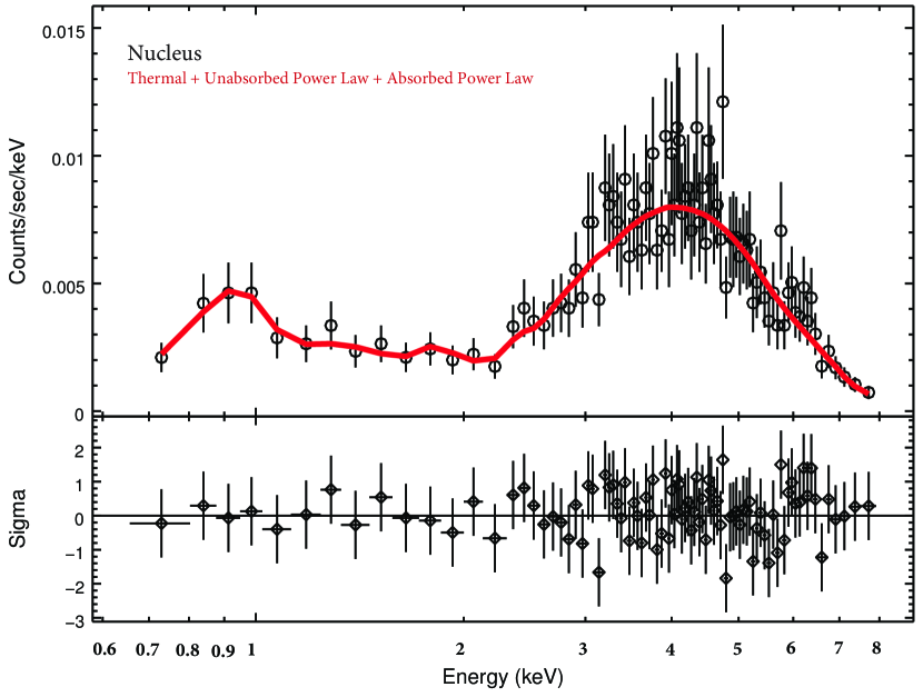
Figure 4.— Spectrum of the nucleus and best-fitting model (absorbed power law + unabsorbed power law + apec thermal model), with the residuals in the lower panel.

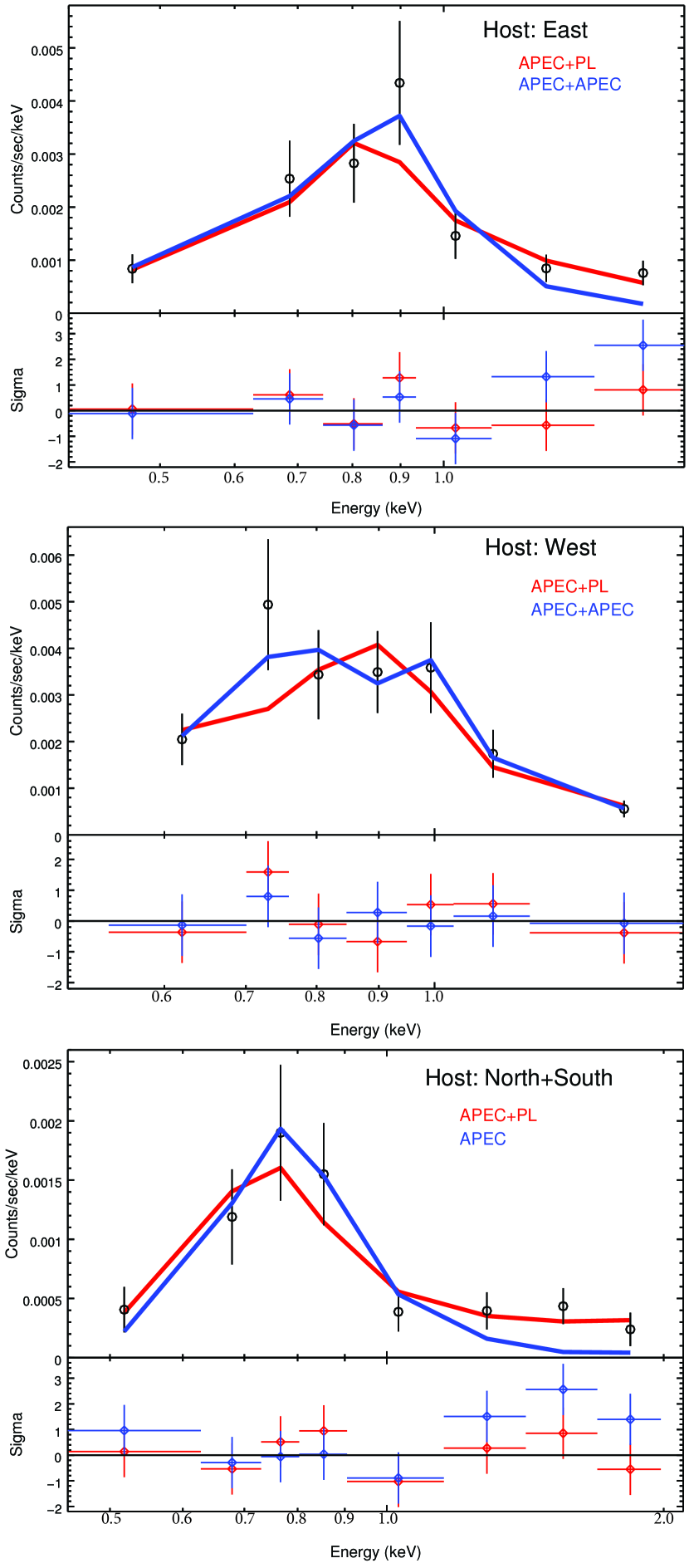
Figure 5.— Spectrum of the host regions: east (top), west (middle), and the sum of north and south (bottom); and best-fitting model (power law + apec thermal model (red) or single or sum of apec models (blue)), with the residuals in the lower panel.

HostE is best modeled as a combination of thermal and power law emission with $\Gamma=2.1$ and a temperature $kT=0.7$ keV (Figure 5 top). Neither a power law nor a thermal model alone are sufficient. While the sum of two thermal models recovers the peak at $\sim 0.9$ keV better than the best model, this model does not fit the 1-2 keV slope. In contrast, hostW is better modeled with the sum of the thermal models ($kT=0.4$ keV and $kT=1.3$ keV; Figure 5 middle), although the sum of a power law and a thermal model is also a good fit ($\Gamma=3.7$ and $kT=1.0$ keV). However, the thermal model recovers the 0.7 keV feature better.

The host galaxy outside of the regions with the jets (hostN+hostS) is best modeled as the sum of a power law ($\Gamma=-0.4$) and an apec thermal model ($kT=0.4$ keV). As in HostE, fits without a power law component recover the peak better but fail to match the 1$-$2 keV slope. The sum of two thermal models is not a significant improvement over a single thermal model, so we only include the single temperature fit in Figure 5 and Table 3. However, the likelihood of these models is low ($p=0.050$).

Photoionized emission is seen from the extended narrow-line regions (NLR) of Seyfert galaxies such as NGC 1068 and NGC 4151 (Ogle et al., 2003, 2000). The nucleus of 3C 293 is a relatively luminous for a low ionization nuclear emission-line region (LINER), so we investigate the possibility that photoionization may contribute to its extended X-ray emission. It is difficult to distinguish between thermal and photoionized plasma at the ACIS-S spectral resolution, even though they emit lines with different relative strengths. A photoionized spectrum can be confirmed by measuring the plasma temperature via narrow recombination continuum widths with a grating spectrograph (Kinkhabwala et al., 2002). Lacking such data, we can test to see if the observed extended emission meets energetic and ionization requirements. The total luminosity of the host(E+W+N+S) extended emission is $2.5\times 10^{41}$ erg s^-1, 2% of the unabsorbed power-law nuclear 0.4-8 keV luminosity of $8.7\times 10^{42}$ erg s^-1. Therefore, we cannot rule out significant photoionized emission by energetics alone. However, photoionization at a projected distance of 13 kpc from the nucleus of 3C 293 would require a very low density, insufficient to produce the observed extended X-ray flux. O vii emission with a characteristic ionization parameter of of $\xi=$L${}_{X}/n_{e}r^{2}=10$ would require an electron density of $\sim 6\times 10^{-4}$ cm^-3, giving a hydrogen column density of only $N_{\mathrm{H}}\sim 2\times 10^{19}$ cm^-2 for a filling factor of unity, which is roughly a factor of 1000 too small to produce the observed extended soft X-ray emission. In contrast, the X-ray NLR of NGC 1068 has a mean column density of $N_{\mathrm{H}}\sim 5\times 10^{22}$ cm^-2 and mean $n_{e}=3.0$ cm^-3 (Ogle et al., 2003). Moreover, from Hi absorption studies, Beswick et al. (2004) revealed column densities of $N_{H}\sim 10^{21}$ cm^-2 (assuming T${}_{\rm spin}=100$ K) for the gas in the central disk that is in front of the radio continuum. We can therefore rule out any significant contribution from photoionization to the extended X-ray emission in 3C 293.

4.3. Large-Scale Jet Features

The spectra of the three features along the large jets (NW1, NW2, and SE1) are shown in Figure 6. Similar to the small-scale jets, we only fit the spectra from 0.4$-$3 keV, which is the range over which there are significant counts. We fit each spectrum with (1) a power law alone and (2) a thermal apec model alone, but with only six data points, there are insufficient degrees of freedom to fit more complex models (e.g. a combination of a power law and a thermal model). We impose a foreground absorber due to the Milky Way ISM and fixed the apec model metallicity to solar.

NW2 is best fit with a power law with $\Gamma=2.5$. A thermal model ($kT=3.3$ keV) is significantly worse ($\chi^{2}$/dof=6.99/4), but it cannot be completely ruled out (probability of 0.14). In contrast, NW1 and SE1 are well fit by either a power law ($\Gamma=1.6$; $\Gamma=1.9$) or a thermal model ($kT=3.6$ keV; $kT=4.3$ keV).

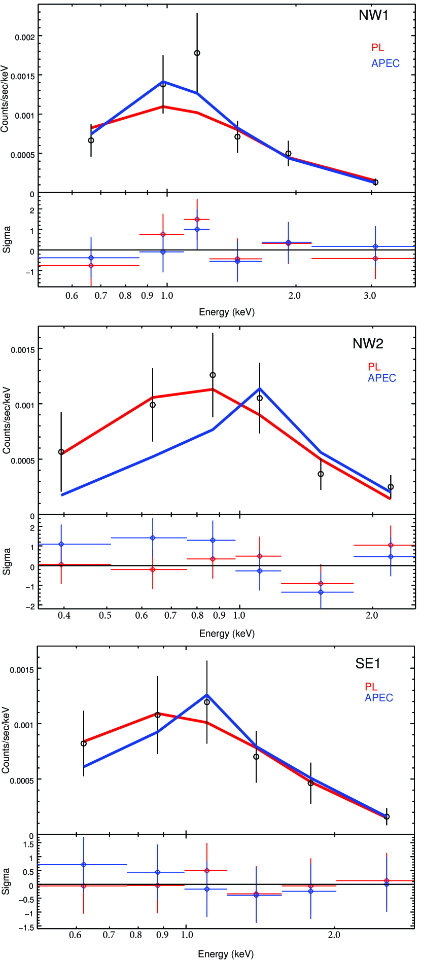
Figure 6.— Spectrum of NW1 (top), NW2 (middle), and SE1 (bottom) and best-fitting model (power law (red) or apec thermal model (blue)), with the residuals in the lower panel.

5. DISCUSSION

Table 4Observed and Derived Parameters

Region	L(0.4$-$8.0 keV)		L(1.4 GHz)	Thermal X-ray Gas
	apec	Power Law		$n_{e}$	Energy	Pressure	$\tau_{\rm cool}$
	(1040 erg/s)		(1040 erg/s)	($f^{-1/2}$cm-3)	($f^{1/2}10^{56}$ erg)	($f^{-1/2}10^{-11}$ erg/cm3)	($f^{1/2}10^{8}$ yr)
Nucleus	2.3	39.1; 874	24.2	0.019	2.2	4.6	4.1
E. Jet	1.7	5.2	13.9	0.0028	6.6	0.49	12.
W. Jet (0.4 keV)	2.8		20.0	0.0036	5.9	0.37	6.7
W. Jet (1.3 keV)	2.6			0.0039	20.	1.3	25.
Host: N+S	1.3	12.2		0.0013	7.4	0.13	18.
NW Jet		11.4	5.2
SE Jet		5.6	1.0

5.1. Jet Power

We measured the kinetic power of the jets from their radio emission in two ways. Punsly (2005) and Shabala & Godfrey (2013) each provide a means of calculating the kinetic power of the jets based on the 151 MHz luminosity and, in the case of the Shabala & Godfrey (2013) the extent of the lobes. We used the 16.08 Jy measurement of Waldram et al. (1996) and a 100 kpc extent of the lobes. These formulae give us a kinetic power of $2-4\times 10^{43}$ erg s^-1, which is 2$-$3 orders of magnitude larger than the radiative power at 1.4 GHz or in the X-ray bands, and more than sufficient to heat the X-ray emitting gas. If this gas exists in thermal equilibrium, $\sim 0.4$% of the kinetic power needs to be dissipated to compensate for radiative losses of $1.1\times 10^{41}$ erg s^-1, assuming these losses are dominated by the soft thermal X-ray emission. If both the power law and thermal components of the X-ray emission observed within the host galaxy are due to dissipated kinetic power, then the amount needed rises to $\sim 1-2$%.

5.2. ISM Emission

5.2.1 Hot ISM

We use the Chandra spectra to characterize the X-ray emitting gas in the host galaxy, which may be heated by the radio jets. From the thermal components of the best fit of the nuclear and host spectra, we calculate the electron density, energy, and cooling timescale of the thermal plasma. The electron density can be calculated directly from the normalization of the apec models (see Table 3). We assume constant density in taking the volume integral and $n_{H}=0.8n_{e}$, which corresponds to a fully ionized plasma with 10% He. We set the nuclear volume to be a sphere with a radius the size of the extraction aperture and the host volumes to be segments of the 20^′′ sphere corresponding to their extraction region (e.g. V${}_{\rm East}=(4/3)\pi(20^{\prime\prime})^{3}\times(55/360)$). The resulting electron densities, given in Table 4, range between $1.3\times 10^{-3}\,{f^{-1/2}\,cm^{-3}}$ and $1.9\times 10^{-2}\,{f^{-1/2}\,cm^{-3}}$, which are reasonable for hot ISM. Based on the thermal emission, we also measure the mass of X-ray emitting gas (Table 5). We find masses of (5, 2, and 8)$\times 10^{8}{f^{1/2}}$ M_⊙ of hot gas in the North+South, East, and West host regions, cooling at a rate of 1.1 M_⊙ yr^-1.

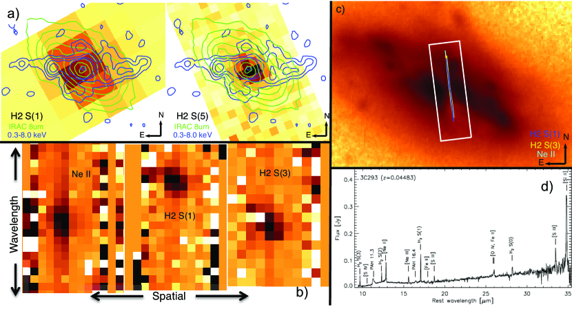
Figure 7.— IRS maps of 3C 293 maps (a) of the H₂ S(1) and H₂ S(5) emission overlaid with contours of 8 $\mu$m (green) and X-ray (blue) emission showing that the H₂ emission is concentrated near the nucleus, but extends over much of the galactic disk. Cut-outs of the staring observation (b) at the H₂ S(1), H₂ S(3), and [Ne ii] lines similarly show that the shocked gas is found over much of the galactic disk (c; B-band image also shown in Fig. 3). The integrated spectrum, previously published in Guillard et al. (2012), is shown in panel (d).

5.2.2 Warm H₂ Emission

Ogle et al. (2010) measured a total luminosity of the H₂ rotational lines $0-0~{}S(0)-S(3)$ of $5.75\times 10^{41}$ erg s^-1. A small percentage ($\sim$1%) of kinetic energy dissipated from the jets is more than sufficient to account for the observed warm H₂ emission. The $3.7\times 10^{9}$ M_⊙ of warm molecular hydrogen at 100 K observed by Ogle et al. (2010) contains 5$\times 10^{52}$ erg of thermal energy, about 4 orders of magnitude smaller than the $\sim 10^{56-57}$ erg contained in the hot ISM, calculated based on its temperature and electron density.

Figure 7 shows the extent of the warm ISM with respect to the thermal X-ray emission. There is a concentration at the center of the galaxy, seen in particular in the H2 S(5) map, but warm H₂ is detected over much of the galactic disk, as shown by the H₂ S(1) map (Fig. 7a). The staring observation also allows us to determine that the [Ne ii], which can also be heated by shocks, is likewise found over most of the length of the SH slit, which covers much of the breadth of the galactic disk.

Table 5Luminous Galaxy Contents

Component	Mass (M⊙)	Temperature
Hot ISM	$1.6\times 10^{9}$	0.4-1.3 keV
Warm H2	$3.7\times 10^{9}$	100-1040 K
Ionized Gas	$7~{}~{}\,\times 10^{5}$
Cold H2	$2.2\times 10^{10}$
Dust	$6.7\times 10^{7}$	20 K and 59 K
Stellar	$1.7\times 10^{11}$

5.2.3 Dust and CO Emission

Figure 8 shows the spectral energy distribution (SED) of the host galaxy measured in a 30^′′ aperture from the UV to FIR. We used the SED modeling code magphys (da Cunha et al., 2008) to fit it and derive properties of the host galaxy. magphys fits SEDs with a stellar spectra library derived from the Bruzual & Charlot (2003) stellar population synthesis code and an infrared dust spectrum, comprised of a polycyclic aromatic hydrocarbon (PAH) template, a MIR continuum at fixed temperatures (130 K and 250 K) and two thermal dust components. The SED fit estimates the dust mass of 3C 293 at $7\pm 3\times 10^{7}$ M_⊙. However, Lanz et al. (2013) and Aniano et al. (2012) both noted that SED fits done in the absence of photometry at $\lambda\geq 170\mu$m, as is the case here, tend to underestimate the cold dust temperature and hence overestimate the dust mass by as much as 60%.

3C 293 was the first FRII galaxy in which CO was detected (Evans et al., 1999). More recent observations by Labiano et al. (2013) determined that CO is distributed in a highly structured, elongated disk extending out to 12^′′ from the nucleus (Fig. 3). These observations also suggest the presence of a CO absorber in front of the AGN, interpreted by Evans et al. (1999) and Labiano et al. (2013) as circumnuclear clouds on noncircular trajectories. 3C 293 contains a total cold H₂ mass of $M(H_{2})=2.2\times 10^{10}$ M_⊙ (Evans et al., 1999; Labiano et al., 2013). Therefore, the gas-to-dust ratio in 3C 293 is $330$. If the dust mass is indeed overestimated due to the limited FIR observations, then this ratio may be even higher. A similar effect is seen in the MOHEG NGC 4258, which has an even greater CO-inferred gas-to-dust ratio of 1000 (Ogle et al., 2014), as well as in the Taffy bridge, which shows an enhancement level similar to 3C 293 (Zhu et al., 2007). However, shocks may enhance the CO emission in 3C 293 (as suggested by the highly excited CO emission found by Papadopoulos et al. (2008)), resulting in an over-estimation of the H₂ mass, if a typical $X_{CO}$ is assumed, as well as the related gas-to-dust ratio. Table 5 also shows that 3C 293 has a warm-to-cold H₂ ratio of $\sim 0.17$.

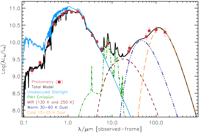
Figure 8.— Integrated SED of the host of 3C 293, using GALEX, SDSS, 2MASS, IRAC, MIPS, and IRAS photometry, fit with magphys. The fitted model requires a stellar mass (blue) of $1.7\times 10^{11}$ M_⊙, and a dust mass of $6.7\times 10^{7}$ M_⊙ primarily at 20 K (orange) and 59 K (purple). The SED was extracted in the 30^′′ circular aperture shown in Figure 3.

5.3. Jet Feedback on the ISM

5.3.1 X-ray Emission in Radio Galaxies

Table 6Comparison Among Galaxies

Galaxy	X-ray Properties					IR Properties
	log(L${}_{\rm X,\,AGN}$	log(LThermal	EThermal	T	Ref.	log(L${}_{\rm 24\mu m,\,AGN}$	log(L${}_{H_{2}}$	Ref.
	(erg s-1))	(erg s-1))	(erg)	(keV)		(erg s-1))	(erg s-1))
3C 293	42.9	41.0	7$\times 10^{56}$	0.7, 1.0	1	43.3	41.8	12
NGC 4258	40.9	39.9	5$\times 10^{55}$	0.5	2, 3	42.7	39.9	1, 13
Cen A	41.7	40	2$\times 10^{56}$	0.3	4, 5	42.7	39.9	12
3C 305	41.2	40.3	6$\times 10^{56}$	0.8	6, 7	43.4	$<$41.4	7
3C 321	43.6	40.7	…	0.3	8	44.9	$<$42.1	12, 14
PKS 1138-26	45.6	45.1	2$\times 10^{61}$	5	1,9	…	44.9	1, 15
NGC 3801	41.5	39.8	5$\times 10^{55}$	0.2-1.0	10	…	…	…
4C 29.30	43.7	42.0	$10^{56-57}$	0.5	11	…	…	…

The presence of thermal X-ray gas associated with radio jets has been identified in a number of radio galaxies (e.g., NGC 4258: Yang et al. 2007; Centaurus A: Kraft et al. 2009; 3C 321: Evans et al. 2008). In several such galaxies, X-ray emission is seen to trace the radio jets but with a wider, resolved region of emission. Wilson et al. (2001) describe the X-ray emission, which Yang et al. (2007) determined to be thermally emitting gas at $\sim 0.5$ keV, as “enveloping” the radio jets that rise to the anomalous arms of NGC 4258. Similarly, Massaro et al. (2009) argue that the diffuse X-ray emission in 3C 305 is observed to surround the radio emission rather than exist solely coincident with it, attributing this thermal emission to gas collisionaly heated by shocks driven by the jets.

3C 305, particularly, has similar morphological and spectral X-ray properties to 3C 293 (Table 6). Both show extended, thermal X-ray emission along the direction of the radio jets out to $\sim$10 kpc from the nucleus. 4C 29.30 (Siemiginowska et al., 2012) and NGC 3801 (Croston et al., 2007; Emonts et al., 2012) likewise show large quantities of thermal X-ray emission associated with the radio jet propagating through their host galaxies. At higher redshift, the Spiderweb galaxy (PKS1138-26, z=2.16; Carilli et al., 2002; Ogle et al., 2012) contains a thermal X-ray cocoon around its radio jets and is an extremely luminous MOHEG. The situation is further complicated in 3C 293 where radio observations (e.g., Beswick et al., 2002; Joshi et al., 2011) have captured either the large $\sim 100$ kpc jets or the small $\sim 5$ kpc jets. However, the flux contained within the small scale radio jets appears to account for the unresolved flux in the core when the large jets are resolved. Therefore, it appears that the X-ray jets do continue $\sim 10$ kpc beyond the inner radio jets, in a region devoid of bright radio emission. This mismatch between the X-ray and radio jets may be a result of a longer cooling timescale for the X-ray emitting cocoon compared to the synchrotron-emitting jets or the faster motion of the radio features in the jet compared to the cocoon.

Observations of more nearby systems with better spatial resolution including NGC 4258 and Centaurus A have produced the picture (e.g., Wilson et al., 2001; Kraft et al., 2007) that radio jets through their interaction with the ISM shock gas to X-ray emitting temperatures. For example, the shell of hot (3.5 keV) gas detected around the SW lobe of Centaurus A (Kraft et al., 2003, 2007) was interpreted as the result of a supersonic expansion of the radio lobe into the surrounding ISM. However, the jet of Centaurus A is much more perpendicular to its host galaxy. NGC 4258, in contrast, has a similar geometry to 3C 293 in that the radio jets initially traverse the denser galactic disk. In the process, they shock the ISM gas. Once the jets leave the main galactic disk, they continue to drive mass motions and shocks through the lower density ISM, creating an expanding cocoon of shocked gas (Sutherland & Bicknell, 2007; Wagner et al., 2012). As a result, while the solid angle of the jet remains small, its area of impact can eventually cover the whole host galaxy. Wilson et al. (2001) suggest that the diffuse emission they measure around the anomalous arms of NGC 4258 is primarily the result of the mass motions directed towards the galactic disk hitting and shocking the disk ISM to X-ray temperatures. This hot gas is also blown out of the disk as a result, creating the emission along the anomalous arms that is particularly bright on the edge closest to the disk.

Applying this picture to 3C 293 implies that the emission observed east and west of the nucleus is likely the result of ISM shocked to X-ray temperatures. The large radio jets could drive mass motions into the galactic disk, shocking gas to further contribute to the observed emission. Only a tiny fraction of the kinetic power of the radio jets ($<1$%) would be necessary to account for the X-ray emission. The morphology of the X-ray emission within the host of 3C 293 further supports this picture, as it hints at similarities to the anomalous arms of NGC 4258. The western jet in particular has a suggestion of a curve towards the larger NW jet, reminiscent of the departure of the anomalous arms of NGC 4258 from the disk of their host galaxy.

5.3.2 Relation of H₂ and Diffuse X-ray Emission

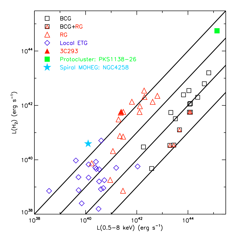
Figure 9.— H₂ luminosity compared to X-ray (0.5-8 keV) luminosity of the host MOHEG galaxies excluding the AGN. The black lines show where L${}_{H_{2}}$/L_X=[1, 0.1, 0.01, 0.0001]. Radio galaxies (red triangles) generally have similar L${}_{H_{2}}$ and L_X, with higher L_X than the typical early type galaxy (ETG; blue diamonds). The filled symbol is 3C 293. Brightest cluster galaxies (BCGs; black squares) have X-ray luminosity associated with the cluster within the host galaxy, so their L_X is approximately two orders of magnitude larger than their L${}_{H_{2}}$.

In this picture, the shocks driven by the jet power both the thermal X-ray emission and the warm H₂ emission. Figure 9 shows the relation between L${}_{H_{2}}$ and the X-ray luminosity of MOHEGs hosted in radio galaxies, brightest cluster galaxies (BCGs) and local early type galaxies (ETGs). The appendix describes how the X-ray luminosity was extracted in detail. In brief, we extracted spectra in the aperture given by the stellar extent, excluding the central hard point source. We find that radio galaxies, including 3C 293, which are not BCGs, have similar L${}_{H_{2}}$ and L_X. In contrast, the X-ray luminosity of BCGs is about two orders of magnitude larger than L${}_{H_{2}}$. We suggest that in the non-BCG radio galaxies both the X-ray and H₂ emission is powered by shocks driven by the jet, whereas in BCGs, the X-ray emission is dominated by cooling in the gravitational potential that has created a well-developed hot atmosphere over periods much longer than the current jet activity. ETGs have a wide range of X-ray luminosities relative to their L${}_{H_{2}}$.

We suggest the following evolutionary interpretation for the locations of different types of galaxies in the plot. When the radio jet is activated, perhaps by a merger, the interaction of the jet with the ISM drives the galaxy up and to the right in Figure 9, as it drives increases in both H₂ and X-ray luminosity. Without energy injection, the H₂ cools more quickly than the hot ISM, moving galaxies downward in the plot. However, as the H₂ emission is dependent on the dissipation of kinetic energy, its cooling occurs on the turbulent dissipation timescale, which can be longer than the time between two active jet phases, as has recently been shown for 3C 326 (Guillard et al. 2014, in press.). The net effect of each cycle of radio jet activity is to drive a galaxy to the right (higher X-ray luminosity).

From the ratio of the H₂ and diffuse, thermal X-ray luminosities, we can extract the ratio of their masses and filling factors ($f$), assuming both gases fill the same volume V. The H₂ luminosity is given by:

$$L_{H_{2}} = \frac{M_{H_{2}}}{2m_{p}}X_{H_{2}}=f_{H_{2}}Vn_{H_{2}}X_{H_{2}}{\rm,where~{}~{}}$$ (1)

$$X_{H_{2}} = 3kT_{H_{2}}/\tau_{H_{2}}~{}.$$ (2)

The bulk of 3C 293 warm H₂ mass ($M_{H_{2}}$) is at a temperature ($T_{H_{2}}$) 100 K (Ogle et al., 2010), where the mean luminosity per molecule $X_{H_{2}}=4.7\times 10^{-26}$ erg/s, and hence the cooling timescale is $\tau_{H_{2}}=3\times 10^{4}$ yr, assuming no constant energy injection into the H₂ gas. The thermal X-ray luminosity is given by:

$$L_{X} = \frac{M_{X}}{m_{p}}n_{e}X_{X}=f_{X}Vn_{e}^{2}X_{X}{\rm,where}$$ (3)

$$X_{X} = 3/2~{}kT_{X}/(n_{e}\tau_{X})~{}.$$ (4)

For the typical temperature $T_{X}$ (0.8 keV) and $n_{e}$ ($3\times 10^{-3}$ cm^-3) of the hot plasma (Table 4), log($X_{X}/({\rm erg~{}s^{-1}~{}cm^{3}}))=-22.5$ (Cox, 2000) and $\tau_{X}=6\times 10^{9}$ yr. The ratio of the H₂ and X-ray luminosities then yields the ratio of filling factors and masses of each gas phase:

$$\frac{L_{H_{2}}}{L_{X}}=\frac{n_{H_{2}}}{n_{e}^{2}}\frac{f_{H_{2}}}{f_{X}}\frac{X_{H_{2}}}{X_{X}}=\frac{M_{H_{2}}}{M_{X}}\frac{X_{H_{2}}}{2n_{e}X_{X}}~{}.$$ (5)

We estimate $n_{H_{2}}$=$1\times 10^{3}$ cm^-3 (Guillard et al. in prep.), so 3C 293’s luminosity ratio of 2.33 yields $f_{H_{2}}/f_{X}=1\times 10^{-5}$ and $M_{H_{2}}/M_{X}=9$, within a factor of a few of the ratio of the masses given in Table 5. Assuming similar densities, radio galaxies, which typically have $L_{H_{2}}/L_{X}\sim 1$, have $f_{H_{2}}/f_{X}\sim 10^{-5}$ and $M_{H_{2}}/M_{X}\sim 4$. The similarities in the luminosities and masses of warm H₂ and thermal X-ray gas are consistent with the picture that in these systems both derive from a multiphase, shocked ISM. In contrast, BCGs whose $L_{H_{2}}/L_{X}\sim 0.01$ have $f_{H_{2}}/f_{X}\sim 10^{-7}$ and $M_{H_{2}}/M_{X}\sim 0.04$, because their massive, virialized, hot atmospheres overwhelm the X-ray emission due to the current jet-ISM interaction. As an intermediary case, the Spiderweb BCG (PKS1138-26), a powerful radio source that resides in an unvirialized protocluster, has $L_{H_{2}}/L_{X}\sim 0.4$.

The X-ray cooling timescale ($\tau_{X}$) is $\sim 10^{5}$ times longer than $\tau_{H_{2}}$, so shock-heated X-ray plasma has more time to spread from the shock sites and fill more of the emitting volume before cooling than the H₂ emission. Over time, jet-ISM interactions may contribute to the establishment of a hot atmosphere in massive ellipticals including BCGs. If the jet operates for 10⁷ yr to generate the observed X-ray luminosity in 3C 293, then it needs to operate either continuously for $10^{9}$ yr or with a duty cycle of 10% for $10^{10}$ yr to generate the X-ray luminosity observed in BCGs. If the energy used by the jet to drive outflows also dissipates in the host, then this process may be even more efficient at generating the hot atmosphere. Alternatively, galaxy interactions, including minor mergers, may also contribute to the buildup of the X-ray atmospheres.

5.3.3 Gas Outflows

Jet feedback on ISM can also drive outflows. 3C 293 is known to house both ionized and neutral gas outflows (Morganti et al., 2003; Emonts et al., 2005; Mahony et al., 2013). In particular, radio observations have detected a broad ($\sim 1200$ km s^-1) neutral HI outflow from the small-scale western radio jet (Mahony et al., 2013; Morganti et al., 2003) and optical spectroscopy detected a fast-moving ionized outflow primarily associated with the small-scale eastern jet (Emonts et al., 2005). These authors have argued that the jets of 3C 293 are capable of driving these outflows. This is further supported by the application of the work of Wagner et al. (2012) to 3C 293. Wagner et al. (2012) used hydrodynamical simulations to determine that radio jets are capable of accelerating ISM clouds to the velocities found in the outflows of 3C 293 by sweeping up material ablated by ram pressure of high-velocity flows in the channels through a porous ISM, provided that the ratio of jet power to Eddington luminosity $\eta=P_{\rm jet}/L_{\rm Edd.}\gtrsim 10^{-4}$. In 3C 293, our measurement of the jet power yields $\eta=0.002$, more than sufficient to accelerate clouds to outflow velocities.

Figure 2 shows the region in which these outflows are being detected. Although the Chandra resolution is significantly coarser than the resolution in the radio, we detect significant soft X-ray counts coincident with Region E0 of Emonts et al. (2005, our region NE0). E0 contains a blue shifted, broad-component emission-line feature seen in [S ii] and [O ii] (with FWHM $\sim 730$ km s^-1 and $\Delta$v$\sim-540$ km s^-1 with respect to the narrow-component emission-line disk), which was interpreted as the base of a fast, ionized outflow. However, the estimate of Emonts et al. (2005) of the spatial extent of this outflow of $2\times 1.5$ kpc² is larger than the extent of the soft X-ray emission, suggesting that we are detecting the X-rays only at the launch site of the outflow. In contrast, the neutral outflow, which launches from the knot in the inner western jet (Beswick et al., 2004), is closer to the AGN and hence, we cannot determine with the resolution of this observation whether it too has X-ray emission associated with its launch site. The absence of such emission might suggest that the same process responsible for the heating the X-ray emitting gas is ionizing the eastern outflowing gas.

The kinetic power of the jet ($\sim(2-4)\times 10^{43}$ erg s^-1; Sect. 5.1) is likely sufficient to power these outflows, even if this path of energy dissipation did not simultaneously help to power the X-ray or H₂ emission. However, a much larger fraction of the kinetic power is needed to drive these outflows than to power the emission. The ionized outflow is estimated to dissipate $\sim 10^{56}$ erg over its 10⁶ yr lifetime, requiring an average $\sim 10^{42}$ erg s^-1 to drive it (Emonts et al., 2005), while the energy loss rate of the more massive neutral outflow estimated by Mahony et al. (2013) is between $1.4\times 10^{42}$ erg s^-1 and $1.0\times 10^{43}$ erg s^-1 based on a mass-flow rate of 8-50 M_⊙ yr^-1. The upper end of the mass flow and energetics estimates of the neutral flow are derived assuming that the entire broad Hi component is due to an outflow at 600 km s^-1. Mahony et al. (2013) argue that a plausible alternative scenario has part of this absorption profile being due to turbulent gas in a rotating disk, resulting in a conservative lower limit of 8 M_⊙ yr^-1 flowing out at 100 km s^-1 with an energy loss rate of $1.4\times 10^{42}$ erg s^-1. This scenario is also similar to that proposed by Beswick et al. (2004) for the intermediate Hi seen against the inner western lobe. The energetics of the jet compared to the outflow also argue for a neutral mass outflow on the lower end of the range given by Mahony et al. (2013). The diffuse X-ray luminosity provides a gauge of the amount of energy dissipated into the host galaxy. At Ṁ$=8$ M_⊙ yr^-1, driving the neutral outflow only requires $\sim 5$% of the jet’s kinetic power ($\sim 10^{42}$ erg s^-1), only a factor of $\sim 4$ larger than the diffuse X-ray luminosity. In contrast, if the neutral outflow has an Ṁ$=50$ M_⊙ yr^-1, then the energy necessary for the jet to drive such an outflow ($\sim 10^{43}$ erg s^-1) would sap much of the kinetic power of the jet.

5.4. Extended Structures

The large-scale radio morphology of 3C 293 is that of an FR ii with lobes of unequal surface brightness. Its associated X-ray features are reminiscent of features seen in Cen A. In particular, the SE1 and NW2 components are similar to the shell of X-ray emission around the southern lobe of Cen A (Kraft et al., 2003). NW1 has some similarity with the thermal knots detected in Cen A’s northern middle lobe (Kraft et al., 2009), but may be the X-ray hotspot associated with the radio peak (Figure 1c).

There are several possible explanations for the X-ray emission from these structures along the large-scale radio jets. It could be direct synchrotron emission, synchrotron self-compton (SSC), or inverse-Compton scattering of cosmic microwave background (IC-CMB) photons off of the radio-synchrotron emitting relativistic electrons of the lobes. Alternatively, it could be the result of the jet colliding with intergalactic medium or material dragged out of the host galaxy in an outflow during a previous outburst. However, it does not appear likely that the jet is colliding with material from the tidal tails. Based on the extended emission seen in the B-band (Figure 3), the bulk of tidal material is roughly perpendicular to the axis of the radio jets in the plane of the sky.

The spectra of the three regions (Fig. 6; Table 3) are consistent with a power law model, making synchrotron, SSC, and IC-CMB emission plausible explanations. The extrapolation of the radio flux, assuming $\alpha=1$, to the predicted X-ray flux due to direct synchrotron emission, yields a ratio of observed-to-predicted X-ray flux of $2-4$ for NW1 and NW2, placing these features in the regime of hotspots where Hardcastle et al. (2004, see esp. their Fig. 2) argued that a synchrotron model is natural. The upper limits from Spitzer and SDSS data do not provide interesting constraints on the synchrotron model. For all three features, the photon energy density is smaller by a large factor ($>$1000) than the energy density in the magnetic fields (Joshi et al., 2011), indicating that the majority of the energy loss happens through synchrotron emission rather than SSC. Given the low-redshift of 3C 293, IC-CMB emission is likewise unlikely to contribute significantly to the observed emission without important beaming effects, which are not indicated by the morphology of 3C 293.

NW1 fits well with either a power-law model or a thermal model. If its emission is due to synchrotron emission, a plausible scenario as described above, then it may be associated with the radio hotspot 6.6 kpc away (Fig. 1c). Assuming a speed of 0.15$c$ (Harwood et al., 2013), the distance between the peak of the X-ray and radio emission would require $\sim 10^{5}$ yr to cross. This is long compared to the synchrotron lifetime for electrons emitting in the X-ray regime ($\sim 10^{3}$ yr in the 11 $\mu$G magnetic field estimated by Joshi et al. (2011)), but short compared to the synchrotron lifetime for electrons emitting in the radio ($\sim 10^{7}$ yr). The longer-lived radio-emitting particles are visible downstream, at a distance that the X-ray emitting particles could not travel in their lifetime. Offsets between radio and X-ray emission have been seen in other radio galaxies (e.g. 3C 390.3 in Hardcastle et al. 2007 and 3C 351 in Hardcastle et al. 2002), and it has been argued that such spatial differences cannot be accounted for with SSC or IC-CMB models without requiring implausibly large spatial variations in the low-energy electron populations and/or important beaming effects.

If the emission in NW1 is thermal instead, then it requires a fairly high temperature of 3.6 keV to explain its emission, and it is morphologically similar to the thermal knots found in the northern middle lobe of Cen A, which were determined by Kraft et al. (2009) to be most likely due to a jet-cloud interaction resulting in shock-heating of cold gas. However, the Cen A knots are noticeably cooler with temperatures between 0.4 keV and 1 keV (Kraft et al., 2009).

In contrast, SE1, and to a lesser degree NW2, have morphologies more reminiscent of a shell or cap of shock-heated X-ray gas around a supersonically expanding radio lobe. SE1 is particularly morphologically reminiscent of the X-ray emission detected along the edge of the southern lobe of Cen A (Kraft et al., 2003). There is also some morphological similarity to the curved feature on the edge of the northern lobe of 4C 29.30 (EArm; Siemiginowska et al., 2012), which, like the Cen A feature, is thermal in origin. Although it does not appear on the end of the SE lobe, Figure 1a shows that stronger radio emission is present on either side of SE1 along the lobe, suggesting this feature may lie at the forefront of an ejection burst, perhaps associated with a bowshock. The spectrum of SE1 is equally well fit with a power-law or a thermal model. In contrast, NW2 is more likely to be synchrotron emission ($\Gamma=2.5$, p=0.68) but we cannot rule out a thermal model (p=0.14). Without a deeper observation, however, we cannot better determine the origin of the emission in these features.

6. SUMMARY

We presented a 70 ks Chandra observation of the radio galaxy 3C 293, which shows evidence for jet-shocked, X-ray emitting gas both within the galaxy and at several locations outside of the galaxy. We find the following:

1. In addition to hard emission from the AGN, the nuclear region contains a softer off-nuclear source associated with the launch site of the ionized outflow.

2. Most of the X-ray emission within the host galaxy has jet-like morphology to the East and West of the nucleus, which is best fit with two thermal models (West) and the combination of a thermal model and a power-law model (East).

3. Diffuse, soft X-ray emission is detected to the North and South of the AGN within the host galaxy and requires both a thermal and power-law component to fit its spectrum.

4. We detect two curved features along the large radio jets: SE1 is reminiscent of the thermal X-ray emission around Cen A’s South Lobe and the north lobe of 4C 29.30, while NW2 is more likely to have synchrotron emission.

5. We also detect a possible X-ray counterpart to the NW jet hotspot, whose emission is plausibly explained by synchrotron emission.

The morphologies and luminosities of 3C 293 fit well into a picture whereby the jet affects the ISM through shocks. The kinetic power of the jet is more than sufficient to power the X-ray thermal emission and the warm H₂ emission as well as driving both the ionized and neutral outflows found in this system. As the jet crosses its host galaxy, it drives shocks into the ISM, heating some of the gas up to X-ray emitting temperatures and creating a cocoon of hot gas. This hot gas then expands in a more spherical manner, thereby bringing the effects of the radio jet to a much larger portion of the host galaxy than the cross-section of the jet itself, and could transfer energy to the H₂ either by driving shocks into dense clouds or through turbulent mixing. Only a small fraction of the kinetic energy of the jets ($<3$%) needs to be dissipated to account for both the thermal X-ray and H₂ emission, well within the range of the efficiency of energy transfer expected from numerical simulations.

We compared the diffuse X-ray luminosity and warm H₂ luminosities in a sample of MOHEGs housed in radio galaxies, BCGs, and local ellipticals. We find that radio galaxies, including 3C 293, have a ratio of H₂ and X-ray luminosities of $\sim 1$. This is consistent with the picture that the shocks driven into the ISM by the radio jet powers both types of emission in these systems. In contrast, BCGs, housed in deeper gravitational wells with longer lasting X-ray halos have $L_{H_{2}}/L_{X}\sim 0.01$. However, multiple jet-ISM interactions may serve to help build up a hot, virtualized atmosphere in these giant galaxies.

Appendix A X-RAY LUMINOSITIES OF MOHEGS

Figure 9 shows the relation between the warm H₂ luminosity and the X-ray luminosity of the host galaxy in MOHEGs, and was discussed in Section 5.3.2. Here we describe the process by which we determined the X-ray luminosity for the objects in this figure. The H₂ luminosities were taken from seven references: Ogle et al. (2010), Guillard et al. (2012), Donahue et al. (2011), Rampazzo et al. (2013), Ogle et al. (2012), Egami et al. (2006), and Roussel et al. (2007). We retrieved the observations listed in Table 7 from the Chandra archive and reprocessed them with using ciao version 4.5 to create a new level 2 events file in the same manner as the 3C 293 observation. We typically used just the longest observation, except in cases where only short observations existed. There we processed the available observations and combined the spectra. We used SDSS images (or 2MASS images where not available) to determine apertures the size of the stellar disk. The apertures were centered on the 5$-$8 keV point central point source. X-ray spectra were extracted using the specextract task over the galactic disk excluding the central AGN. In the cases where we extracted spectra from multiple observations of the same galaxy, we combined them at this point. Each spectrum was fit with thermal (apec) or power law models to determine the 0.5$-$8 keV luminosities, given in Table 8. For the six sources with insufficient counts to fit a spectrum, we use the tool WebPIMMS to estimate the luminosity, assuming an APEC model with a temperature similar to that derived from fits to galaxies with similar hardness ratios: (logT=6.95 or kT=0.768 keV for 3C 315, 3C 326, 3C 424, and 3C 459; logT=7.05, kT=0.967 keV for 3C 436; logT=7.65, kT=3.849 keV for NGC 5273). The galaxies typically fall into one of three types: radio galaxies, brightest cluster galaxies, and local early type galaxies. The exceptions are indicated on Figure 9.

Table 3Parameters of X-ray Spectral Fits

Region	Model	Parameters		Luminosity
		Name	Value	Component	Range (keV)	(1040 erg s-1)
Nucleus	(1*)	Photon Indexabs.	1.32$\pm$0.36	Power Law	0.4$-$8.0	$874^{+128}_{-277}$
		$S_{\rm PL,1\,keV,abs.}{\rm(nJy)}$	148${}^{+81}_{-77}$	(absorbed)	0.4$-$2.0	$271^{+156}_{-144}$
		NH (1022 cm-2)	9.41$\pm$1.84		2.0$-$8.0	$567^{+61}_{-118}$
		Photon Indexunabs.	0.57$\pm$0.87	Power Law	0.4$-$8.0	$39.1^{+37.1}_{-16.5}$
		$S_{\rm PL,1\,keV,unabs.}{\rm(nJy)}$	2.46${}^{+1.00}_{-1.03}$	(unabsorbed)	0.4$-$2.0	$4.96^{+1.87}_{-1.54}$
					2.0$-$8.0	$36.4^{+40.0}_{-15.7}$
		$kT{\rm(keV)}$	1.03$\pm$0.10	Thermal (apec)	0.4$-$8.0	$2.33^{+0.65}_{-0.69}$
		N${}_{\textsc{apec}}{\rm(10^{-6}\,cm^{-5})}$	2.08$\pm$0.66		0.4$-$2.0	$2.15^{+0.60}_{-0.62}$
		$\chi^{2}$/dof	48.39/86		2.0$-$8.0	$0.16^{+0.08}_{-0.07}$
	(2)	Photon Index	0.50$\pm$0.22	Power Law	0.4$-$8.0	$558^{+28}_{-70}$
		$S_{PL,1\,keV}{\rm(nJy)}$	32.81${}^{+12.45}_{-12.73}$		0.4$-$2.0	$65.4^{+21.6}_{-23.3}$
		NH (1022 cm-2)	4.44$\pm$0.77		2.0$-$8.0	$486^{+25}_{-50}$
		$\chi^{2}$/dof	165.5/90
NC	(2*)	Photon Index	0.77$\pm$0.24	Power Law	0.4$-$8.0	$739^{+48}_{-146}$
		$S_{PL,1\,keV}{\rm(nJy)}$	$63.6^{+24.2}_{-26.1}$		0.4$-$2.0	$122^{+44}_{-47}$
		NH (1022 cm-2)	6.28$\pm$0.93		2.0$-$8.0	$604^{+35}_{-74}$
		$\chi^{2}$/dof	70.73/76
NE0	(3*)	Photon Index	0.67$\pm$0.20	Power Law	0.4$-$8.0	$34.5^{+6.9}_{-5.9}$
		$S_{PL,1\,keV}{\rm(nJy)}$	$2.61^{+0.44}_{-0.47}$		0.4$-$2.0	$5.03^{+0.70}_{-0.85}$
		$\chi^{2}$/dof	3.02/5		2.0$-$8.0	$29.5^{+7.3}_{-5.7}$
Host: East	(3)	Photon Index	2.22$\pm$0.27	Power Law	0.4$-$8.0	7.30${}^{+1.37}_{-1.11}$
		$S_{PL,1\,keV}{\rm(nJy)}$	2.33${}^{+0.28}_{-0.26}$		0.4$-$2.0	4.60${}^{+0.40}_{-0.72}$
		$\chi^{2}$/dof	11.73/5		2.0$-$8.0	2.78${}^{+1.32}_{-0.92}$
	(4*)	Photon Index	2.10$\pm$0.52	Power Law	0.4$-$8.0	$5.20^{+2.95}_{-1.37}$
		$S_{PL,1\,keV}{\rm(nJy)}$	1.47${}^{+0.50}_{-0.35}$		0.4$-$2.0	$3.01^{+0.86}_{-0.99}$
					2.0$-$8.0	$2.94^{+4.31}_{-1.14}$
		$kT{\rm(keV)}$	0.74$\pm$0.16	Thermal (apec)	0.4$-$8.0	$1.71^{+0.71}_{-0.68}$
		N${}_{\textsc{apec}}{\rm(10^{-6}\,cm^{-5})}$	1.29$\pm$0.50		0.4$-$2.0	$1.65^{+0.45}_{-0.79}$
		$\chi^{2}$/dof	3.73/ 3		2.0$-$8.0	$0.050^{+0.059}_{-0.031}$
	(5)	$kT{\rm(keV)}$	0.23$\pm$0.11	Thermal (apec)	0.4$-$8.0	$1.48^{+1.11}_{-0.97}$
		N${}_{\textsc{apec}}{\rm(10^{-6}\,cm^{-5})}$	2.17$\pm$0.88	(0.23 keV)	0.4$-$2.0	$1.48^{+1.06}_{-0.99}$
					2.0$-$8.0	$0.0005^{+0.0043}_{-0.0005}$
		$kT{\rm(keV)}$	0.96$\pm$0.16	Thermal (apec)	0.4$-$8.0	$2.66^{+0.76}_{-0.72}$
		N${}_{\textsc{apec}}{\rm(10^{-6}\,cm^{-5})}$	2.23$\pm$0.65	(0.96 keV)	0.4$-$2.0	$2.52^{+0.79}_{-0.72}$
		$\chi^{2}$/dof	10.25/3		2.0$-$8.0	$0.15^{+0.04}_{-0.04}$
Host: West	(3)	Photon Index	3.24$\pm$0.31	Power Law	0.4$-$8.0	$7.84^{+0.98}_{-0.96}$
		$S_{PL,1\,keV}{\rm(nJy)}$	2.65${}^{+0.35}_{-0.33}$		0.4$-$2.0	$7.10^{+0.85}_{-0.99}$
		$\chi^{2}$/dof	13.72/5		2.0$-$8.0	$0.85^{+0.39}_{-0.29}$
	(4)	Photon Index	3.70$\pm$0.88	Power Law	0.4$-$8.0	$4.47^{+1.76}_{-1.65}$
		$S_{PL,1\,keV}{\rm(nJy)}$	1.36${}^{+0.58}_{-0.62}$		0.4$-$2.0	$4.14^{+1.43}_{-1.50}$
					2.0$-$8.0	$0.27^{+0.68}_{-0.22}$
		$kT{\rm(keV)}$	0.97$\pm$0.13	Thermal (apec)	0.4$-$8.0	$2.42^{+0.80}_{-0.89}$
		N${}_{\textsc{apec}}{\rm(10^{-6}\,cm^{-5})}$	2.09$\pm$0.80		0.4$-$2.0	$2.25^{+0.73}_{-0.73}$
		$\chi^{2}$/dof	3.87/3		2.0$-$8.0	$0.15^{+0.09}_{-0.07}$
	(5*)	$kT{\rm(keV)}$	0.42$\pm$0.12	Thermal (apec)	0.4$-$8.0	$2.76^{+0.71}_{-0.85}$
		N${}_{\textsc{apec}}{\rm(10^{-6}\,cm^{-5})}$	2.63$\pm$0.81	(0.42 keV)	0.4$-$2.0	$2.74^{+0.65}_{-0.68}$
					2.0$-$8.0	$0.016^{+0.017}_{-0.012}$
		$kT{\rm(keV)}$	1.34$\pm$0.13	Thermal (apec)	0.4$-$8.0	$2.58^{+0.76}_{-0.77}$
		N${}_{\textsc{apec}}{\rm(10^{-6}\,cm^{-5})}$	3.11$\pm$0.85	(1.34 keV)	0.4$-$2.0	$2.20^{+0.65}_{-0.64}$
		$\chi^{2}$/dof	1.10/3		2.0$-$8.0	$0.38^{+0.12}_{-0.12}$
Host: North+South	(3)	Photon Index	2.22$\pm$0.39	Power Law	0.4$-$8.0	$3.11^{+0.81}_{-0.54}$
		$S_{PL,1\,keV}{\rm(nJy)}$	$0.99^{+0.15}_{-0.15}$		0.4$-$2.0	$1.91^{+0.31}_{-0.28}$
		$\chi^{2}$/dof	13.52/6		2.0$-$8.0	$1.20^{+0.80}_{-0.52}$
	(4*)	Photon Index	-0.37$\pm$1.64	Power Law	0.4$-$8.0	$12.19^{+46.07}_{-9.17}$
		$S_{PL,1\,keV}{\rm(nJy)}$	$0.30^{+0.21}_{-0.16}$		0.4$-$2.0	$0.72^{+0.28}_{-0.32}$
					2.0$-$8.0	$11.42^{+42.22}_{-9.35}$
		$kT{\rm(keV)}$	0.39$\pm$0.08	Thermal (apec)	0.4$-$8.0	1.31${}^{+0.31}_{-0.32}$
		N${}_{\textsc{apec}}{\rm(10^{-6}\,cm^{-5})}$	1.34$\pm$0.42		0.4$-$2.0	1.31${}^{+0.26}_{-0.32}$
		$\chi^{2}$/dof	3.63/4		2.0$-$8.0	0.0056${}^{+0.0043}_{-0.0033}$
	(6)	$kT{\rm(keV)}$	0.57$\pm$0.09	Thermal (apec)	0.4$-$8.0	$1.54^{+0.24}_{-0.25}$
		N${}_{\textsc{apec}}{\rm(10^{-6}\,cm^{-5})}$	1.21$\pm$0.19		0.4$-$2.0	$1.52^{+0.22}_{-0.23}$
		$\chi^{2}$/dof	12.59/6		2.0$-$8.0	$0.022^{+0.011}_{-0.009}$
NW1	(3)	Photon Index	1.63$\pm$0.24	Power Law	0.4$-$8.0	$7.05^{+1.53}_{-1.14}$
		$S_{PL,1\,keV}{\rm(nJy)}$	1.50${}^{+0.21}_{-0.22}$		0.4$-$2.0	$2.84^{+0.42}_{-0.41}$
		$\chi^{2}$/dof	3.85/4		2.0$-$8.0	$4.14^{+1.54}_{-1.06}$
	(6*)	$kT{\rm(keV)}$	3.58$\pm$1.24	Thermal (apec)	0.4$-$8.0	$5.85^{+1.40}_{-1.19}$
		N${}_{\textsc{apec}}{\rm(10^{-6}\,cm^{-5})}$	8.07$\pm$1.41		0.4$-$2.0	$2.98^{+0.40}_{-0.38}$
		$\chi^{2}$/dof	1.65/4		2.0$-$8.0	$2.94^{+1.05}_{-1.19}$
NW2	(3*)	Photon Index	2.51$\pm$0.40	Power Law	0.4$-$8.0	$4.36^{+0.88}_{-0.74}$
		$S_{PL,1\,keV}{\rm(nJy)}$	1.48${}^{+0.22}_{-0.23}$		0.4$-$2.0	$3.04^{+0.55}_{-0.50}$
		$\chi^{2}$/dof	2.31/4		2.0$-$8.0	$1.20^{+0.89}_{-0.52}$
	(6)	$kT{\rm(keV)}$	3.26$\pm$0.92	Thermal (apec)	0.4$-$8.0	$4.16^{+1.30}_{-1.13}$
		N${}_{\textsc{apec}}{\rm(10^{-6}\,cm^{-5})}$	5.96$\pm$1.54		0.4$-$2.0	$2.24^{+0.42}_{-0.43}$
		$\chi^{2}$/dof	6.99/4		2.0$-$8.0	$1.97^{+0.93}_{-0.84}$
SE1	(3*)	Photon Index	1.88$\pm$0.37	Power Law	0.4$-$8.0	$5.64^{+1.87}_{-1.07}$
		$S_{PL,1\,keV}{\rm(nJy)}$	1.45$\pm$0.22		0.4$-$2.0	$2.80^{+0.48}_{-0.47}$
		$\chi^{2}$/dof	0.39/4		2.0$-$8.0	$2.78^{+1.84}_{-1.09}$
	(6)	$kT{\rm(keV)}$	4.29$\pm$1.12	Thermal (apec)	0.4$-$8.0	$5.43^{+1.32}_{-1.35}$
		N${}_{\textsc{apec}}{\rm(10^{-6}\,cm^{-5})}$	7.29$\pm$1.43		0.4$-$2.0	$2.52^{+0.40}_{-0.40}$
		$\chi^{2}$/dof	0.95/4		2.0$-$8.0	$2.93^{+0.94}_{-0.93}$

Table 7Chandra Observations of MOHEGs

Galaxy	Type	Instrument	OID	Exposure	Date	Aperture
				(ks)		RA(J2000)	Dec(J2000)	Size	AGN
3C 31	RG	ACIS-S	2147	44.41	2000-11-06	01:07:24.959	$+$32:24:45.21	$~{}\,30^{\prime\prime}\times~{}\,25^{\prime\prime}$(320∘)	$2\farcs 5$
3C 84	BCG/RG	ACIS-S	4952	164.24	2004-10-14	03:19:48.160	$+$41:30:42.11	$80^{\prime\prime}$	$2\farcs 5$
3C 218	BCG/RG	ACIS-S	4970	98.82	2004-10-22	09:18:05.688	$-$12:05:43.39	$20^{\prime\prime}$	$2\farcs 5$
3C 236	RG	ACIS-I	10249	40.50	2009-01-14	10:06:01.735	$+$34:54:10.43	$20^{\prime\prime}$	$2\farcs 5$
		ACIS-I	10246	29.38	2009-03-10
3C 270	RG	ACIS-S	9569	100.00	2008-02-12	12:19:23.245	$+$05:49:29.63	$100^{\prime\prime}$	$2\farcs 5$
3C 272.1	RG	ACIS-S	5908	46.08	2005-05-01	12:25:03.707	$+$12:53:12.92	$125^{\prime\prime}$	$2\farcs 5$
3C 293	RG	ACIS-S	12712	67.81	2010-11-16	13:52:17.821	$+$31:26:46.50	$30^{\prime\prime}$	$2\farcs 5$
3C 305	RG	ACIS-S	12797	28.66	2011-01-03	14:49:21.625	$+$63:16:14.43	$40^{\prime\prime}$	$2\farcs 5$
3C 310	RG	ACIS-S	11845	57.58	2010-04-09	15:04:57.179	$+$26:00:58.33	$~{}\,9^{\prime\prime}$	$1\farcs 0$
3C 315	RG	ACIS-S	9313	7.67	2007-12-10	15:13:40.096	$+$26:07:31.86	$~{}\,5^{\prime\prime}$	$1\farcs 0$
3C 317	BCG/RG	ACIS-S	5807	126.95	2006-03-24	15:16:44.498	$+$07:01:17.62	$35^{\prime\prime}$	$2\farcs 5$
3C 321	RG	ACIS-S	3138	47.13	2010-02-19	15:31:43.492	$+$24:04:18.96	$18^{\prime\prime}$	$1\farcs 5\tablenotemark{d}$
3C 326	RG	ACIS-I	10242	27.51	2009-05-07	15:52:09.140	$+$20:05:47.24	$14^{\prime\prime}$	$1\farcs 0$
		ACIS-I	10908	18.30	2009-05-10
3C 338	BCG/RG	ACIS-I	10748	40.58	2009-11-19	16:28:38.202	$+$39:33:04.70	$45^{\prime\prime}$	$2\farcs 5$
3C 386	RG	ACIS-I	10232	29.29	2008-11-29	18:38:26.251	$+$17:11:49.94	$25^{\prime\prime}$	$1\farcs 5$
3C 405	BCG/RG	ACIS-I	5831	51.09	2005-02-16	19:59:28.296	$+$40:44:01.99	$25^{\prime\prime}$	$2\farcs 5$
3C 424	RG	ACIS-S	12743	7.95	2011-04-15	20:48:12.099	$+$07:01:17.05	$10^{\prime\prime}$	$1\farcs 0$
3C 433	RG	ACIS-S	7881	37.17	2007-08-28	21:23:44.565	$+$25:04:27.56	$20^{\prime\prime}$	$2\farcs 5$
3C 436	RG	ACIS-S	9318	8.04	2008-01-08	21:44:11.700	$+$28:10:19.00	$10^{\prime\prime}$	$1\farcs 5$
		ACIS-S	12745	7.95	2011-05-27
3C 459	RG	ACIS-S	12734	7.95	2011-10-13	23:16:35.230	$+$04:05:18.50	$10^{\prime\prime}$	$1\farcs 0$
4C 12.50	RG	ACIS-S	836	25.35	2000-02-24	13:47:33.360	$+$12:17:24.04	$20^{\prime\prime}$	$2\farcs 0$
IC 5063	RG	ACIS-S	7878	34.10	2007-06-15	20:52:02.402	$-$57:04:07.58	$100^{\prime\prime}\times~{}\,50^{\prime\prime}$(295∘)	$2\farcs 5$
NGC 4258	Spiral	ACIS-S	350	14.04	2000-04-17	12:18:57.518	$+$47:18:14.38	$250^{\prime\prime}\times 100^{\prime\prime}$(335∘)	$4\farcs 0$
		ACIS-S	1618	22.00	2001-05-28
Donahue et al. (2011)
2A0335+096	BCG	ACIS-S	9792	33.74	2007-12-20	03:38:40.861	$+$09:57:57.17	$25^{\prime\prime}$	$2\farcs 0$
		ACIS-S	7939	49.54	2007-12-16
Abell 478	BCG	ACIS-S	1669	42.39	2001-01-27	04:13:25.300	$+$10:27:54.49	$14^{\prime\prime}$	$1\farcs 0$
Abell 1068	BCG	ACIS-S	1652	26.84	2001-02-04	10:40:44.499	$+$39:57:11.13	$~{}\,15^{\prime\prime}\times~{}7\farcs 5$(320∘)	$1\farcs 0$
Abell 1795	BCG	ACIS-S	493	19.63	2001-04-27	13:48:52.505	$+$26:35:34.59	$10^{\prime\prime}$	$1\farcs 0$
		ACIS-S	494	19.52	2001-01-12
Abell 1835	BCG	ACIS-I	6880	117.92	2006-08-25	14:01:02.081	$+$02:52:42.34	$~{}\,7^{\prime\prime}$	$1\farcs 0$
Abell 2597	BCG	ACIS-S	7329	60.11	2006-05-04	23:25:19.735	$-$12:07:27.18	$15^{\prime\prime}$	$1\farcs 0$
MS0735.6+7421	BCG	ACIS-I	10470	141.96	2009-06-16	07:41:44.346	$+$74:14:39.44	$10^{\prime\prime}$	$1\farcs 0$
PKS 0745-19	BCG	ACIS-S	12881	118.07	2011-01-27	07:47:31.325	$-$19:17:40.35	$12^{\prime\prime}$	$1\farcs 0$
Rampazzo et al. (2013)
IC 1459	ETG	ACIS-S	2196	58.83	2001-08-12	22:57:10.607	$-$36:27:44.20	$120^{\prime\prime}\times~{}\,90^{\prime\prime}$($275^{\circ}$)	$2\farcs 5$
NGC 1052	ETG	ACIS-S	5910	59.20	2005-09-18	02:41:04.839	$-$08:15:20.75	$~{}\,75^{\prime\prime}\times~{}\,50^{\prime\prime}$($300^{\circ}$)	$2\farcs 5$
NGC 4036	ETG	ACIS-S	6783	13.72	2006-07-24	12:01:26.753	$+$61:53:44.81	R:$68^{\prime\prime}\times 69^{\prime\prime}$($255^{\circ}$)	$1\farcs 5$
NGC 4477	ETG	ACIS-S	9527	37.68	2008-04-27	12:30:02.198	$+$13:38:11.77	$~{}\,90^{\prime\prime}\times~{}\,80^{\prime\prime}$($195^{\circ}$)	$1\farcs 5$
NGC 4550	ETG	ACIS-S	8050	5.09	2008-02-19	12:35:30.622	$+$12:13:15.11	$~{}\,70^{\prime\prime}\times~{}\,20^{\prime\prime}$($359^{\circ}$)	$1\farcs 0$
		ACIS-S	8058	5.50	2008-02-18
		ACIS-S	8098	5.09	2008-02-24
NGC 4697	ETG	ACIS-S	784	39.26	2000-01-15	12:48:35.878	$-$05:48:02.56	$110^{\prime\prime}\times~{}\,70^{\prime\prime}$($250^{\circ}$)	$2\farcs 0$
		ACIS-S	4727	39.92	2003-12-26
		ACIS-S	4728	35.68	2004-01-06
		ACIS-S	4729	38.10	2004-02-12
		ACIS-S	4730	40.05	2004-08-18
NGC 5018	ETG	ACIS-S	2070	30.89	2001-04-14	13:13:01.032	$-$19:31:05.65	$~{}\,60^{\prime\prime}\times~{}\,45^{\prime\prime}$($275^{\circ}$)	$1\farcs 5$
NGC 5044	ETG	ACIS-S	9399	82.68	2008-03-07	13:15:23.945	$-$16:23:07.33	$72^{\prime\prime}$	$1\farcs 5$
NGC 5077	ETG	ACIS-S	11780	28.68	2010-05-09	13:19:31.651	$-$12:39:25.21	$~{}\,50^{\prime\prime}\times~{}\,40^{\prime\prime}$($190^{\circ}$)	$1\farcs 0$
NGC 5273	ETG	ACIS-S	415	1.73	2000-09-03	13:42:08.354	$+$35:39:15.28	$~{}\,70^{\prime\prime}\times~{}\,60^{\prime\prime}$($190^{\circ}$)	$1\farcs 5$
NGC 5353	ETG	ACIS-I	5903	4.49	2005-04-10	13:53:26.693	$+$40:16:58.91	$~{}\,50^{\prime\prime}\times~{}\,25^{\prime\prime}$($325^{\circ}$)	$1\farcs 5$
NGC 6868	ETG	ACIS-I	3191	23.46	2002-11-01	20:09:54.014	$-$48:22:46.72	$~{}\,80^{\prime\prime}\times~{}\,60^{\prime\prime}$($280^{\circ}$)	$1\farcs 5$
		ACIS-I	11753	72.60	2009-08-19
Kaneda et al. (2008)
NGC 708	BCG	ACIS-S	7921	110.67	2006-11-20	01:52:46.480	$+$36:09:06.60	$~{}\,40^{\prime\prime}$	$1\farcs 5$
NGC 1395	ETG	ACIS-I	799	27.37	1999-12-31	03:38:29.873	$-$23:01:38.90	$75^{\prime\prime}$	$1\farcs 5$
NGC 1549	ETG	ACIS-S	2077	36.53	2000-11-08	04:15:45.175	$-$55:35:32.37	$~{}\,80^{\prime\prime}\times~{}\,90^{\prime\prime}$(270∘)	$1\farcs 5$
NGC 3557	ETG	ACIS-I	3217	37.49	2002-11-28	11:09:57.642	$-$37:32:20.96	$~{}\,70^{\prime\prime}\times~{}\,50^{\prime\prime}$(210∘)	$1\farcs 5$
NGC 3894	ETG	ACIS-S	10389	38.54	2009-07-20	11:48:50.306	$+$59:24:56.38	$~{}\,60^{\prime\prime}\times~{}\,40^{\prime\prime}$(200∘)	$1\farcs 5$
NGC 4696	BCG	ACIS-S	2931	9.63	2002-09-21	21:18:33.025	$+$26:26:49.03	$~{}\,60^{\prime\prime}\times~{}\,40^{\prime\prime}$(245∘)	$2\farcs 0$
NGC 4589	ETG	ACIS-S	6785	13.77	2006-08-31	12:37:24.871	$+$74:11:30.92	R:$110^{\prime\prime}\times 65^{\prime\prime}$(300∘)	$1\farcs 0$
NGC 7052	ETG	ACIS-S	4954	89.05	2004-04-01	12:48:49.250	$-$41:18:39.00	$~{}\,45^{\prime\prime}\times~{}\,35^{\prime\prime}$(275∘)	$2\farcs 0$
Ogle et al. (2012), Egami et al. (2006), Alatalo et al. (2011)
PKS 1138-26	PC	ACIS-S	898	39.47	2000-06-06	11:40:48.353	$-$26:29:08.52	$~{}\,10^{\prime\prime}$	$1\farcs 0$
Z3146	BCG	ACIS-I	909	46.01	2000-05-10	10:23:39.600	$+$04:11:10.00	$~{}\,10^{\prime\prime}$	$2\farcs 0$
NGC 1266	ETG	ACIS-S	11578	29.65	2009-09-20	03:16:00.769	$-$02:25:38.54	$~{}\,40^{\prime\prime}\times~{}\,30^{\prime\prime}$(108∘)	$1\farcs 5$

Table 8MOHEGs Parameters

Galaxy	D	Log(L${}_{H_{2}}$	Ref.	Log(LAGN	Ref.	Host X-ray Emission
	(Mpc)	(erg/s))		(erg/s))		Counts	Model	Model	Log(LX
				(2-10 keV)		(0.5-8 kev)		Parameters	(erg/s))
3C 31	74	40.32	(1)	40.67	(1)	1754	M1	kT=0.91 keV	41.07
								$\Gamma=1.94$
3C 84	76	41.75	(1)	42.91	(1)	3434419	M2	kT1=0.93 keV	44.10
								kT2=3.93 keV
3C 218	245	41.10	(1)	41.69	(1)	99092	M2	kT1=0.78 keV	43.67
								kT2=3.69 keV
3C 236	462	41.76	(2)	43.02	(2)	102	M3	$\Gamma=0.21$	42.11
3C 270	32∗	39.26	(1)	41.08	(1)	14218	M2	kT1=0.78 keV	40.96
								kT2=5.72 keV
3C 272.1	18∗	38.86	(1)	39.34	(1)	16732	M2	kT1=0.74 keV	41.46
								kT2=6.84 keV
3C 293	199	41.76	(1)	42.78	(1)	634	M2	kT=0.39 keV	41.39
								kT2=4.94 keV
3C 305	185	$<$41.48	(2)	41.23	(2)	373	M5	kT=0.98 keV	41.29
3C 310	240	40.85	(1)	40.11	(10)	580	M4	kT=1.21 keV	41.47
								Z=0.27
3C 315	501	41.76	(1)	41.68	(1)	11			41.47
3C 317	152	40.53	(1)	41.30	(1)	159379	M2	kT1=1.24 keV	43.30
								kT2=2.91 keV
3C 321	441	42.13	(1)	42.08	(1)	305	M1	kT=0.21 keV	41.81
								$\Gamma=2.95$
3C 326	409	41.73	(1)	40.63	(1)	48			41.37
3C 338	133	40.54	(1)	40.30	(1)	53675	M4	kT=3.48 keV	43.45
								Z=0.84
3C 386	73	39.87	(1)	39.75	(1)	97	M5	kT=1.53 keV	40.24
3C 405	251	41.75	(1)	44.28	(1)	49694	M5	kT=4.76 keV	44.06
3C 424	595	41.97	(1)	42.44	(11)	34			42.12
3C 433	468	42.13	(1)	43.90	(1)	301	M1	kT=0.93 keV	42.62
								$\Gamma=0.37$
3C 436	1000	42.31	(1)	43.53	(1)	36			42.30
3C 459	1090	$<$42.35	(2)	43.24	(2)	46			42.80
4C 12.50	577	42.54	(2)	43.34	(2)	160	M1	kT=0.75 keV	42.29
								$\Gamma=0.54$
IC 5063	49	$<$40.88	(2)	42.97	(2)	1085	M1	kT=0.71 keV	41.34
								$\Gamma=-1.08$
NGC 4258	7.2#	40.59	(3)	40.86	(3)	23365	M6	kT1=0.24 keV	40.10
								kT2=0.74 keV
								Z2=0.19
2A0335+096	153	41.51∗	(4)	$<$40.81	(12)	127023	M7	kT1=2.49 keV	43.51
								kT2=1.03 keV
								NH,kT2=4.2${\rm E}$21 cm-2
Abell 478	392	42.07∗	(4)	$<$41.77	(12)	33502	M8	kT=4.15 keV	44.10
								NH=1.9${\rm E}$21 cm-2
Abell 1068	654	$<$42.55∗	(4)	$<$43.43	(13)	10794	M2	kT1=1.37 keV	44.04
								kT2=3.65 keV
Abell 1795	284	41.74∗	(4)	$<$41.24	(12)	15521	M2	kT1=4.22 keV	43.33
								kT2=1.04 keV
Abell 1835	1272	$<$42.80∗	(4)	$<$42.78	(12)	25290	M5	kT=4.63 keV	44.64
Abell 2597	373	42.39∗	(4)	$<$41.58	(12)	40046	M6	kT1=1.06 keV	43.83
								kT2=3.06 keV
								Z2=0.49
MS0735.6+7421	1068	42.05∗	(4)	$<$42.11	(12)	11505	M5	kT1=3.85 keV	44.07
PKS 0745-19	474	42.30∗	(4)	42.11	(12)	80110	M1	kT1=4.01 keV	44.38
								$\Gamma=1.98$
IC 1459	29∗	39.25	(5)	40.87	(14)	6363	M1	kT1=0.59 keV	40.73
								$\Gamma=2.09$
NGC 1052	19∗	39.83∗	(5)	41.20	(14)	2661	M1	kT1=0.61 keV	40.12
								$\Gamma=1.73$
NGC 4036	24+	39.97||	(5)	39.08	(14)	197	M2	kT1=0.78 keV	39.62
								kT2=0.11 keV
NGC 4477	22+	39.35∗	(5)	39.81	(15)∗	2060	M2	kT1=0.25 keV	40.12
								kT2=0.68 keV
NGC 4550	16∗	38.86||	(5)	$<$38.36	(14)	92	M1	kT1=0.31 keV	38.57
								$\Gamma=0.89$
NGC 4697	12∗	38.40	(5)	38.40	(14)	13670	M1	kT1=0.32 keV	39.85
								$\Gamma=1.73$
NGC 5018	45+	39.66	(5)	$<$39.52	(14)	822	M1	kT1=0.56 keV	40.42
								$\Gamma=2.35$
NGC 5044	31∗	39.72	(5)	39.44	(14)	169214	M2	kT1=2.05 keV	40.38
								kT2=0.91 keV
NGC 5077	40+	39.76	(5)	39.73	(16)	710	M1	kT1=0.80 keV	42.03
								$\Gamma=2.37$
NGC 5273	17∗	38.88#	(5)	40.55	(14)	35			39.73
NGC 5353	36+	38.96	(5)	$<$39.78	i	209	M2	kT1=5.09 keV	40.69
								kT2=0.75 keV
NGC 6868	27∗	39.65∗	(5)	$<$39.98	(17)	4357	M1	kT1=0.75 keV	40.53
								$\Gamma=1.96$
NGC 708	70	40.47+	(6)	$<$39.02	(12)	68804	M6	kT1=1.06 keV	42.26
								kT2=2.02 keV
								Z2=1.73
NGC 1395	24∗	38.92+	(6)	39.06	(14)	2252	M1	kT1=0.84 keV	40.60
								$\Gamma=1.82$
NGC 1549	20∗	38.20+	(6)	38.46	(14)	1055	M3	$\Gamma=1.42$	40.51
NGC 3557	45	$<$39.20+	(6)	40.22	(14)	433	M1	kT1=0.74 keV	40.53
								$\Gamma=1.91$
NGC 3894	45	39.93+	(6)	40.72	(18)	706	M1	kT1=0.33 keV	40.40
								$\Gamma=1.81$
NGC 4589	22∗	39.36+	(6)	38.90	(14)	257	M1	kT1=0.71 keV	39.72
								$\Gamma=2.30$
NGC 4696	36∗	39.68+	(6)	40.00	(14)	386482	M6	kT1=1.08 keV	42.58
								kT2=2.53 keV
								Z2=2.79
NGC 7052	68	39.71+	(6)	$<$40.29	(14)	690	M1	kT1=0.64 keV	41.20
								$\Gamma=2.55$
PKS 1138-26	17346	44.92||	(7)	45.60	(19)	164	M3	$\Gamma=1.10$	45.14
Z3146	1510	43.20∗	(8)	42.91	(1)	10749	M5	kT=4.71 keV	44.18
NGC 1266	29.9||	40.71	(9)	39.53	j	711	M9	kT=0.78 keV	40.61
								$\Gamma=4.24$
								N${}_{\rm H}=4.1{\rm E}$21 cm-2

References

- Ahn et al. (2014) Ahn, C. P., Alexandroff, R., Allende Prieto, C., et al. 2014, ApJS, 211, 17
- Akujor et al. (1996) Akujor, C. E., Leahy, J. P., Garrington, S. T., et al. 1996, MNRAS, 278, 1
- Alatalo et al. (2011) Alatalo, K., Blitz, L., Young, L. M., et al. 2011, ApJ, 735, 88
- Aniano et al. (2012) Aniano, G., Draine, B. T., Calzetti, D., et al. 2012, ApJ, 756, 138
- Appleton et al. (2006) Appleton, P. N., Xu, K. C., Reach, W., et al. 2006, ApJ, 639, L51
- Beswick et al. (2004) Beswick, R. J., Peck, A. B., Taylor, G. B., & Giovannini, G. 2004, MNRAS, 352, 49
- Beswick et al. (2002) Beswick, R. J., Pedlar, A., & Holloway, A. J. 2002, MNRAS, 329, 620
- Bruzual & Charlot (2003) Bruzual, G., & Charlot, S. 2003, MNRAS, 344, 1000
- Cappi et al. (2006) Cappi, M., Panessa, F., Bassani, L., et al. 2006, A&A, 446, 459
- Carilli et al. (2002) Carilli, C. L., Harris, D. E., Pentericci, L., et al. 2002, ApJ, 567, 781
- Combes et al. (2013) Combes, F., García-Burillo, S., Casasola, V., et al. 2013, A&A, 558, A124
- Cox (2000) Cox, A. N. 2000, Allen’s astrophysical quantities (Springer)
- Crenshaw et al. (2003) Crenshaw, D. M., Kraemer, S. B., & George, I. M. 2003, ARA&A, 41, 117
- Croston et al. (2007) Croston, J. H., Kraft, R. P., & Hardcastle, M. J. 2007, ApJ, 660, 191
- da Cunha et al. (2008) da Cunha, E., Charlot, S., & Elbaz, D. 2008, MNRAS, 388, 1595
- Dasyra & Combes (2012) Dasyra, K. M., & Combes, F. 2012, A&A, 541, L7
- Dasyra et al. (2014) Dasyra, K. M., Combes, F., Novak, G. S., et al. 2014, A&A, 565, A46
- de Vaucouleurs et al. (1991) de Vaucouleurs, G., de Vaucouleurs, A., Corwin, Jr., H. G., et al. 1991, Third Reference Catalogue of Bright Galaxies (New York: Springer)
- Di Matteo et al. (2005) Di Matteo, T., Springel, V., & Hernquist, L. 2005, Nature, 433, 604
- Dicken et al. (2010) Dicken, D., Tadhunter, C., Axon, D., Robinson, A., Morganti, R., & Kharb, P. 2010, ApJ, 722, 1333
- Donahue et al. (2011) Donahue, M., de Messières, G. E., O’Connell, R. W., et al. 2011, ApJ, 732, 40
- Egami et al. (2006) Egami, E., Rieke, G. H., Fadda, D., & Hines, D. C. 2006, ApJ, 652, L21
- Emonts (2006) Emonts, B. H. C. 2006, PhD thesis, University of Groningen
- Emonts et al. (2012) Emonts, B. H. C., Burnett, C., Morganti, R., & Struve, C. 2012, MNRAS, 421, 1421
- Emonts et al. (2010) Emonts, B. H. C., Morganti, R., Struve, C., et al. 2010, MNRAS, 406, 987
- Emonts et al. (2005) Emonts, B. H. C., Morganti, R., Tadhunter, C. N., et al. 2005, MNRAS, 362, 931
- Evans et al. (1999) Evans, A. S., Sanders, D. B., Surace, J. A., & Mazzarella, J. M. 1999, ApJ, 511, 730
- Evans et al. (2008) Evans, D. A., Fong, W.-F., Hardcastle, M. J., et al. 2008, ApJ, 675, 1057
- Fanaroff & Riley (1974) Fanaroff, B. L., & Riley, J. M. 1974, MNRAS, 167, 31P
- Fazio et al. (2004) Fazio, G. G., Hora, J. L., Allen, L. E., et al. 2004, ApJS, 154, 10
- Fischer et al. (2010) Fischer, J., Sturm, E., González-Alfonso, E., et al. 2010, A&A, 518, L41
- Floyd et al. (2006) Floyd, D. J. E., Perlman, E., Leahy, J. P., et al. 2006, ApJ, 639, 23
- Fukazawa et al. (2006) Fukazawa, Y., Botoya-Nonesa, J. G., Pu, J., Ohto, A., & Kawano, N. 2006, ApJ, 636, 698
- García-Burillo et al. (2014) García-Burillo, S., Combes, F., Usero, A., et al. 2014, A&A, 567, A125
- Golombek et al. (1988) Golombek, D., Miley, G. K., & Neugebauer, G. 1988, AJ, 95, 26
- Guillard et al. (2012) Guillard, P., Ogle, P. M., Emonts, B. H. C., et al. 2012, ApJ, 747, 95
- Gültekin et al. (2012) Gültekin, K., Cackett, E. M., Miller, J. M., et al. 2012, ApJ, 749, 129
- Hardcastle et al. (2002) Hardcastle, M. J., Birkinshaw, M., Cameron, R. A., et al. 2002, ApJ, 581, 948
- Hardcastle et al. (2007) Hardcastle, M. J., Croston, J. H., & Kraft, R. P. 2007, ApJ, 669, 893
- Hardcastle et al. (2004) Hardcastle, M. J., Harris, D. E., Worrall, D. M., & Birkinshaw, M. 2004, ApJ, 612, 729
- Hardcastle et al. (2012) Hardcastle, M. J., Massaro, F., Harris, D. E., et al. 2012, MNRAS, 424, 1774
- Harwood et al. (2013) Harwood, J. J., Hardcastle, M. J., Croston, J. H., & Goodger, J. L. 2013, MNRAS, 435, 3353
- Holt et al. (2008) Holt, J., Tadhunter, C. N., & Morganti, R. 2008, MNRAS, 387, 639
- Houck et al. (2004) Houck, J. R., Roellig, T. L., van Cleve, J., et al. 2004, ApJS, 154, 18
- Joshi et al. (2011) Joshi, S. A., Nandi, S., Saikia, D. J., Ishwara-Chandra, C. H., & Konar, C. 2011, MNRAS, 414, 1397
- Kalberla et al. (2005) Kalberla, P. M. W., Burton, W. B., Hartmann, D., et al. 2005, A&A, 440, 775
- Kaneda et al. (2008) Kaneda, H., Onaka, T., Sakon, I., et al. 2008, ApJ, 684, 270
- Kinkhabwala et al. (2002) Kinkhabwala, A., Sako, M., Behar, E., et al. 2002, ApJ, 575, 732
- Kraft et al. (2012) Kraft, R. P., Birkinshaw, M., Nulsen, P. E. J., et al. 2012, ApJ, 749, 19
- Kraft et al. (2000) Kraft, R. P., Forman, W., Jones, C., et al. 2000, ApJ, 531, L9
- Kraft et al. (2009) Kraft, R. P., Forman, W. R., Hardcastle, M. J., et al. 2009, ApJ, 698, 2036
- Kraft et al. (2007) Kraft, R. P., Nulsen, P. E. J., Birkinshaw, M., et al. 2007, ApJ, 665, 1129
- Kraft et al. (2003) Kraft, R. P., Vázquez, S. E., Forman, W. R., et al. 2003, ApJ, 592, 129
- Labiano et al. (2013) Labiano, A., García-Burillo, S., Combes, F., et al. 2013, A&A, 549, A58
- Lacy et al. (2004) Lacy, M., et al. 2004, ApJS, 154, 166
- Lanz et al. (2013) Lanz, L., Zezas, A., Brassington, N., et al. 2013, ApJ, 768, 90
- Lehnert et al. (2011) Lehnert, M. D., Tasse, C., Nesvadba, N. P. H., Best, P. N., & van Driel, W. 2011, A&A, 532, L3
- Mahony et al. (2013) Mahony, E. K., Morganti, R., Emonts, B. H. C., Oosterloo, T. A., & Tadhunter, C. 2013, MNRAS, 435, L58
- Makovoz & Khan (2005) Makovoz, D., & Khan, I. 2005, in Astronomical Society of the Pacific Conference Series, Vol. 347, Astronomical Data Analysis Software and Systems XIV, ed. P. Shopbell, M. Britton, & R. Ebert, 81
- Martin et al. (2005) Martin, D. C., Fanson, J., Schiminovich, D., et al. 2005, ApJ, 619, L1
- Massaro et al. (2009) Massaro, F., Chiaberge, M., Grandi, P., et al. 2009, ApJ, 692, L123
- Massaro et al. (2012) Massaro, F., Tremblay, G. R., Harris, D. E., et al. 2012, ApJS, 203, 31
- More (1978) More, J. J. 1978, in Lecture Notes in Mathematics 630: Numerical Analysis, ed. Watson, G. A. (Berlin: Springer-Verlag), 105–116
- Morganti et al. (2013) Morganti, R., Frieswijk, W., Oonk, R. J. B., Oosterloo, T., & Tadhunter, C. 2013, A&A, 552, L4
- Morganti et al. (2003) Morganti, R., Oosterloo, T. A., Emonts, B. H. C., et al. 2003, ApJ, 593, L69
- Morganti et al. (2005) Morganti, R., Tadhunter, C. N., & Oosterloo, T. A. 2005, A&A, 444, L9
- Nyland et al. (2013) Nyland, K., Alatalo, K., Wrobel, J. M., et al. 2013, ApJ, 779, 173
- Ogle et al. (2007) Ogle, P., Antonucci, R., Appleton, P. N., & Whysong, D. 2007, ApJ, 668, 699
- Ogle et al. (2010) Ogle, P., Boulanger, F., Guillard, P., et al. 2010, ApJ, 724, 1193
- Ogle et al. (2012) Ogle, P., Davies, J. E., Appleton, P. N., et al. 2012, ApJ, 751, 13
- Ogle et al. (2003) Ogle, P. M., Brookings, T., Canizares, C. R., Lee, J. C., & Marshall, H. L. 2003, A&A, 402, 849
- Ogle et al. (2014) Ogle, P. M., Lanz, L., & Appleton, P. N. 2014, ApJ, 788, L33
- Ogle et al. (2000) Ogle, P. M., Marshall, H. L., Lee, J. C., & Canizares, C. R. 2000, ApJ, 545, L81
- Papadopoulos et al. (2008) Papadopoulos, P. P., Kovacs, A., Evans, A. S., & Barthel, P. 2008, A&A, 491, 483
- Park et al. (2006) Park, T., Kashyap, V. L., Siemiginowska, A., et al. 2006, ApJ, 652, 610
- Pellegrini (2010) Pellegrini, S. 2010, ApJ, 717, 640
- Peterson et al. (2012) Peterson, B. W., Appleton, P. N., Helou, G., et al. 2012, ApJ, 751, 11
- Punsly (2005) Punsly, B. 2005, ApJ, 623, L9
- Rampazzo et al. (2013) Rampazzo, R., Panuzzo, P., Vega, O., et al. 2013, MNRAS, 432, 374
- Rieke et al. (2004) Rieke, G. H., Young, E. T., Engelbracht, C. W., et al. 2004, ApJS, 154, 25
- Roussel et al. (2007) Roussel, H., Helou, G., Hollenbach, D. J., et al. 2007, ApJ, 669, 959
- Russell et al. (2013) Russell, H. R., McNamara, B. R., Edge, A. C., et al. 2013, MNRAS, 432, 530
- Scharwächter et al. (2013) Scharwächter, J., McGregor, P. J., Dopita, M. A., & Beck, T. L. 2013, MNRAS, 429, 2315
- Shabala & Godfrey (2013) Shabala, S. S., & Godfrey, L. E. H. 2013, ApJ, 769, 129
- Siemiginowska et al. (2012) Siemiginowska, A., Stawarz, Ł., Cheung, C. C., et al. 2012, ApJ, 750, 124
- Silk & Rees (1998) Silk, J., & Rees, M. J. 1998, A&A, 331, L1
- Skrutskie et al. (2006) Skrutskie, M. F., Cutri, R. M., Stiening, R., et al. 2006, AJ, 131, 1163
- Smith et al. (2007) Smith, J. D. T., Armus, L., Dale, D. A., et al. 2007, PASP, 119, 1133
- Smith et al. (2001) Smith, R. K., Brickhouse, N. S., Liedahl, D. A., & Raymond, J. C. 2001, ApJ, 556, L91
- Solomon et al. (1987) Solomon, P. M., Rivolo, A. R., Barrett, J., & Yahil, A. 1987, ApJ, 319, 730
- Sturm et al. (2011) Sturm, E., González-Alfonso, E., Veilleux, S., et al. 2011, ApJ, 733, L16
- Sutherland & Bicknell (2007) Sutherland, R. S., & Bicknell, G. V. 2007, ApJS, 173, 37
- Theureau et al. (2007) Theureau, G., Hanski, M. O., Coudreau, N., Hallet, N., & Martin, J.-M. 2007, A&A, 465, 71
- Tonry et al. (2001) Tonry, J. L., Dressler, A., Blakeslee, J. P., et al. 2001, ApJ, 546, 681
- Ueda et al. (2005) Ueda, Y., Ishisaki, Y., Takahashi, T., Makishima, K., & Ohashi, T. 2005, ApJS, 161, 185
- Wagner & Bicknell (2011) Wagner, A. Y., & Bicknell, G. V. 2011, ApJ, 728, 29
- Wagner et al. (2012) Wagner, A. Y., Bicknell, G. V., & Umemura, M. 2012, ApJ, 757, 136
- Waldram et al. (1996) Waldram, E. M., Yates, J. A., Riley, J. M., & Warner, P. J. 1996, MNRAS, 282, 779
- Weisskopf et al. (2000) Weisskopf, M. C., Tananbaum, H. D., Van Speybroeck, L. P., & O’Dell, S. L. 2000, in Society of Photo-Optical Instrumentation Engineers (SPIE) Conference Series, Vol. 4012, X-Ray Optics, Instruments, and Missions III, ed. J. E. Truemper & B. Aschenbach, 2–16
- Werner et al. (2004) Werner, M. W., Roellig, T. L., Low, F. J., et al. 2004, ApJS, 154, 1
- Wilson et al. (2001) Wilson, A. S., Yang, Y., & Cecil, G. 2001, ApJ, 560, 689
- Wise et al. (2004) Wise, M. W., McNamara, B. R., & Murray, S. S. 2004, ApJ, 601, 184
- Yang et al. (2007) Yang, Y., Li, B., Wilson, A. S., & Reynolds, C. S. 2007, ApJ, 660, 1106
- Young & Wilson (2004) Young, A. J., & Wilson, A. S. 2004, ApJ, 601, 133
- Zhu et al. (2007) Zhu, M., Gao, Y., Seaquist, E. R., & Dunne, L. 2007, AJ, 134, 118