Probing texture zeros with scaling ansatz in inverse seesaw

Ambar Ghosal111ambar.ghosal@saha.ac.in, Rome Samanta222rome.samanta@saha.ac.in,
Saha Institute of Nuclear Physics, 1/AF Bidhannagar, Kolkata 700064, India
Abstract

We investigate neutrino mass matrix phenomenology involving scaling ansatz and texture zeros adhering inverse seesaw mechanism. It is seen that four is the maximum number of zeros in mDsubscript𝑚𝐷m_{D} and μ𝜇\mu to obtain viable phenomenology. Depending upon the generic nature of the effective neutrino mass matrices we classify all the emerged matrices in four categories. One of them is ruled out phenomenologically due to inappropriate value of reactor mixing angle after breaking of the scaling ansatz. The mass ordering is inverted in all cases. One of the distinguishable feature of all these categories is the vanishingly small value of CP violation measure JCPsubscript𝐽𝐶𝑃J_{CP} due to small value of δCPsubscript𝛿𝐶𝑃\delta_{CP}. Thus those categories will be ruled out if CP violation is observed in the leptonic sector in future experiments.

1 Introduction

Among the variants of the seesaw mechanism, inverse seesaw [1, 2, 3, 4, 5, 6, 7, 8, 9, 10, 11, 12, 13] stands out as an attractive one due to its characteristic feature of generation of small neutrino mass without invoking high energy scale in the theory. Although to realize such feature one has to pay the price in terms of incorporation of additional singlet fermions, nevertheless, in different GUT models accommodation of such type of neutral fermions are natural. Furthermore, such mechanism appeals to the foreseeable collider experiments to be testified due to its unique signature. The 9×9999\times 9 neutrino mass matrix in this mechanism is written as

mνsubscript𝑚𝜈\displaystyle m_{\nu} =\displaystyle= (0mD0mDT0MRS0MRSTμ)matrix0subscript𝑚𝐷0superscriptsubscript𝑚𝐷𝑇0subscript𝑀𝑅𝑆0superscriptsubscript𝑀𝑅𝑆𝑇𝜇\displaystyle\begin{pmatrix}0&m_{D}&0\\ m_{D}^{T}&0&M_{RS}\\ 0&M_{RS}^{T}&\mu\\ \end{pmatrix} (1.1)

with the choice of basis (νL,νRc,SL)subscript𝜈𝐿superscriptsubscript𝜈𝑅𝑐subscript𝑆𝐿(\nu_{L},\nu_{R}^{c},S_{L}). The three matrices appear in mνsubscript𝑚𝜈m_{\nu} are mDsubscript𝑚𝐷m_{D}, MRSsubscript𝑀𝑅𝑆M_{RS} and μ𝜇\mu among them mDsubscript𝑚𝐷m_{D} and MRSsubscript𝑀𝑅𝑆M_{RS} are Dirac type whereas μ𝜇\mu is Majorana type mass matrix. After diagonalization, the low energy effective neutrino mass comes out as

mνsubscript𝑚𝜈\displaystyle m_{\nu} =\displaystyle= mDMRS1μ(mDMRS1)Tsubscript𝑚𝐷superscriptsubscript𝑀𝑅𝑆1𝜇superscriptsubscript𝑚𝐷superscriptsubscript𝑀𝑅𝑆1𝑇\displaystyle m_{D}M_{RS}^{-1}\mu(m_{D}M_{RS}^{-1})^{T} (1.2)
=\displaystyle= FμFT𝐹𝜇superscript𝐹𝑇\displaystyle F\mu F^{T}

where F=mDMRS1𝐹subscript𝑚𝐷superscriptsubscript𝑀𝑅𝑆1F=m_{D}M_{RS}^{-1}. Such definition resembles the above formula as a conventional type-I seesaw expression of mνsubscript𝑚𝜈m_{\nu}. However, mνsubscript𝑚𝜈m_{\nu} contains large number of parameters and it is possible to fit them with neutrino oscillation experimental data [14, 15, 16] (but the predictability is less). Our goal in this work is to find out a phenomenologically viable texture of mDsubscript𝑚𝐷m_{D} and μ𝜇\mu with minimum number of parameters or equivalently maximum number of zeros. We bring together two theoretical ideas to find out a minimal texture and they are
i) Scaling ansatz[17, 18, 19, 20, 21, 22, 23, 24, 25, 26, 27],
ii) Texture Zeros[28, 29, 30, 31, 32, 33, 34, 35, 36, 37, 38, 39, 40, 41, 42, 43, 44, 45].
At the outset of the analysis, we choose a basis where the charged lepton mass matrix (mEsubscript𝑚𝐸m_{E}) and MRSsubscript𝑀𝑅𝑆M_{RS} are diagonal along with texture zeros in mDsubscript𝑚𝐷m_{D} and μ𝜇\mu matrices. We also start by assuming the scaling property in the elements of mDsubscript𝑚𝐷m_{D} and μ𝜇\mu to reduce the number of relevant matrices. Although, we are not addressing the explicit origin of such choice of matrices, however, qualitatively we can assume that this can be achieved due to some flavour symmetry [46] which is required to make certain that the texture zeros appear in mDsubscript𝑚𝐷m_{D} and μ𝜇\mu are in the same basis in which mEsubscript𝑚𝐸m_{E} and MRSsubscript𝑀𝑅𝑆M_{RS} are diagonal. We restrict ourselves within the frame work of SU(2)L×U(1)Y𝑆𝑈subscript2𝐿𝑈subscript1𝑌SU(2)_{L}\times U(1)_{Y} gauge group however, explicit realization of such scheme obviously more elusive which will be studied elsewhere.

2 Scaling property and texture zeros

We consider scaling property between the second and third row of mDsubscript𝑚𝐷m_{D} matrix and the same for μ𝜇\mu matrix also. Explicitly the relationships are written as

(mD)2i(mD)3isubscriptsubscript𝑚𝐷2𝑖subscriptsubscript𝑚𝐷3𝑖\displaystyle\frac{(m_{D})_{2i}}{(m_{D})_{3i}} =\displaystyle= k1subscript𝑘1\displaystyle k_{1} (2.1)
(μ)2i(μ)3isubscript𝜇2𝑖subscript𝜇3𝑖\displaystyle\frac{(\mu)_{2i}}{(\mu)_{3i}} =\displaystyle= k2subscript𝑘2\displaystyle k_{2} (2.2)

where i=1,2,3𝑖123i=1,2,3 is the column index. We would like to mention that although we have considered different scale factors for mDsubscript𝑚𝐷m_{D} and μ𝜇\mu matrices, however, the effective mνsubscript𝑚𝜈m_{\nu} is still scale invariant and leads to θ13=0subscript𝜃130\theta_{13}=0. Thus, it is obvious to further break the scaling ansatz. In order to generate nonzero θ13subscript𝜃13\theta_{13} it is necessary to break the ansatz in mDsubscript𝑚𝐷m_{D} since, breaking in μ𝜇\mu does not affect the generation of nonzero θ13subscript𝜃13\theta_{13} although in some cases it provides m30subscript𝑚30m_{3}\neq 0. In our scheme texture zero format is robust and it remains intact while the scaling ansatz is explicitly broken. Such a scenario can be realized by considering the scaling ansatz and texture zeros to have a different origin.
Another point is to be noted that, since the μ𝜇\mu matrix is complex symmetric whereas mDsubscript𝑚𝐷m_{D} is asymmetric, the scale factor considered in μ𝜇\mu matrix is different from that of mDsubscript𝑚𝐷m_{D} to keep the row wise invariance as dictated by Eqn.(2.1) (for mDsubscript𝑚𝐷m_{D}), and Eqn.(2.2) (for μ𝜇\mu). Finally, since the texture of MRSsubscript𝑀𝑅𝑆M_{RS} matrix is diagonal it is not possible to accommodate scaling ansatz considered in the present scheme.
Let us now turn to further constrain the matrices assuming zeros in different entries. Since, in our present scheme the matrix MRSsubscript𝑀𝑅𝑆M_{RS} is diagonal, we constrain the other two matrices. We start with the maximal zero textures with scaling ansatz of general 3×3333\times 3 matrices and list different cases systematically in Table 1.

Table 1: Texture zeros with scaling ansatz of a general 3×3333\times 3 matrix
777 zero texture
m17=(000k1c100c100)superscriptsubscript𝑚17matrix000subscript𝑘1subscript𝑐100subscript𝑐100m_{1}^{7}=\begin{pmatrix}0&0&0\\ k_{1}c_{1}&0&0\\ c_{1}&0&0\\ \end{pmatrix} m27=(0000k1c200c20)superscriptsubscript𝑚27matrix0000subscript𝑘1subscript𝑐200subscript𝑐20m_{2}^{7}=\begin{pmatrix}0&0&0\\ 0&k_{1}c_{2}&0\\ 0&c_{2}&0\\ \end{pmatrix} m37=(00000k1c300c3)superscriptsubscript𝑚37matrix00000subscript𝑘1subscript𝑐300subscript𝑐3m_{3}^{7}=\begin{pmatrix}0&0&0\\ 0&0&k_{1}c_{3}\\ 0&0&c_{3}\\ \end{pmatrix}
666 zero texture
m16=(d100k1c100c100)superscriptsubscript𝑚16matrixsubscript𝑑100subscript𝑘1subscript𝑐100subscript𝑐100m_{1}^{6}=\begin{pmatrix}d_{1}&0&0\\ k_{1}c_{1}&0&0\\ c_{1}&0&0\\ \end{pmatrix} m26=(0d20k1c100c100)superscriptsubscript𝑚26matrix0subscript𝑑20subscript𝑘1subscript𝑐100subscript𝑐100m_{2}^{6}=\begin{pmatrix}0&d_{2}&0\\ k_{1}c_{1}&0&0\\ c_{1}&0&0\\ \end{pmatrix} m36=(00d3k1c100c100)superscriptsubscript𝑚36matrix00subscript𝑑3subscript𝑘1subscript𝑐100subscript𝑐100m_{3}^{6}=\begin{pmatrix}0&0&d_{3}\\ k_{1}c_{1}&0&0\\ c_{1}&0&0\\ \end{pmatrix}
m46=(d1000k1c200c20)superscriptsubscript𝑚46matrixsubscript𝑑1000subscript𝑘1subscript𝑐200subscript𝑐20m_{4}^{6}=\begin{pmatrix}d_{1}&0&0\\ 0&k_{1}c_{2}&0\\ 0&c_{2}&0\\ \end{pmatrix} m56=(0d200k1c200c20)superscriptsubscript𝑚56matrix0subscript𝑑200subscript𝑘1subscript𝑐200subscript𝑐20m_{5}^{6}=\begin{pmatrix}0&d_{2}&0\\ 0&k_{1}c_{2}&0\\ 0&c_{2}&0\\ \end{pmatrix} m66=(00d30k1c200c20)superscriptsubscript𝑚66matrix00subscript𝑑30subscript𝑘1subscript𝑐200subscript𝑐20m_{6}^{6}=\begin{pmatrix}0&0&d_{3}\\ 0&k_{1}c_{2}&0\\ 0&c_{2}&0\\ \end{pmatrix}
m76=(d10000k1c300c3)superscriptsubscript𝑚76matrixsubscript𝑑10000subscript𝑘1subscript𝑐300subscript𝑐3m_{7}^{6}=\begin{pmatrix}d_{1}&0&0\\ 0&0&k_{1}c_{3}\\ 0&0&c_{3}\\ \end{pmatrix} m86=(0d2000k1c300c3)superscriptsubscript𝑚86matrix0subscript𝑑2000subscript𝑘1subscript𝑐300subscript𝑐3m_{8}^{6}=\begin{pmatrix}0&d_{2}&0\\ 0&0&k_{1}c_{3}\\ 0&0&c_{3}\\ \end{pmatrix} m96=(00d300k1c300c3)superscriptsubscript𝑚96matrix00subscript𝑑300subscript𝑘1subscript𝑐300subscript𝑐3m_{9}^{6}=\begin{pmatrix}0&0&d_{3}\\ 0&0&k_{1}c_{3}\\ 0&0&c_{3}\\ \end{pmatrix}
555 zero texture
m15=(000k1c1k1c20c1c20)superscriptsubscript𝑚15matrix000subscript𝑘1subscript𝑐1subscript𝑘1subscript𝑐20subscript𝑐1subscript𝑐20m_{1}^{5}=\begin{pmatrix}0&0&0\\ k_{1}c_{1}&k_{1}c_{2}&0\\ c_{1}&c_{2}&0\\ \end{pmatrix} m25=(000k1c10k1c3c10c3)superscriptsubscript𝑚25matrix000subscript𝑘1subscript𝑐10subscript𝑘1subscript𝑐3subscript𝑐10subscript𝑐3m_{2}^{5}=\begin{pmatrix}0&0&0\\ k_{1}c_{1}&0&k_{1}c_{3}\\ c_{1}&0&c_{3}\\ \end{pmatrix} m35=(0000k1c1k1c30c1c3)superscriptsubscript𝑚35matrix0000subscript𝑘1subscript𝑐1subscript𝑘1subscript𝑐30subscript𝑐1subscript𝑐3m_{3}^{5}=\begin{pmatrix}0&0&0\\ 0&k_{1}c_{1}&k_{1}c_{3}\\ 0&c_{1}&c_{3}\\ \end{pmatrix}
m45=(d1d20k1c100c100)superscriptsubscript𝑚45matrixsubscript𝑑1subscript𝑑20subscript𝑘1subscript𝑐100subscript𝑐100m_{4}^{5}=\begin{pmatrix}d_{1}&d_{2}&0\\ k_{1}c_{1}&0&0\\ c_{1}&0&0\\ \end{pmatrix} m55=(0d2d3k1c100c100)superscriptsubscript𝑚55matrix0subscript𝑑2subscript𝑑3subscript𝑘1subscript𝑐100subscript𝑐100m_{5}^{5}=\begin{pmatrix}0&d_{2}&d_{3}\\ k_{1}c_{1}&0&0\\ c_{1}&0&0\\ \end{pmatrix} m65=(d10d3k1c100c100)superscriptsubscript𝑚65matrixsubscript𝑑10subscript𝑑3subscript𝑘1subscript𝑐100subscript𝑐100m_{6}^{5}=\begin{pmatrix}d_{1}&0&d_{3}\\ k_{1}c_{1}&0&0\\ c_{1}&0&0\\ \end{pmatrix}
m75=(d1d200k1c200c20)superscriptsubscript𝑚75matrixsubscript𝑑1subscript𝑑200subscript𝑘1subscript𝑐200subscript𝑐20m_{7}^{5}=\begin{pmatrix}d_{1}&d_{2}&0\\ 0&k_{1}c_{2}&0\\ 0&c_{2}&0\\ \end{pmatrix} m85=(0d2d30k1c200c20)superscriptsubscript𝑚85matrix0subscript𝑑2subscript𝑑30subscript𝑘1subscript𝑐200subscript𝑐20m_{8}^{5}=\begin{pmatrix}0&d_{2}&d_{3}\\ 0&k_{1}c_{2}&0\\ 0&c_{2}&0\\ \end{pmatrix} m95=(d10d30k1c200c20)superscriptsubscript𝑚95matrixsubscript𝑑10subscript𝑑30subscript𝑘1subscript𝑐200subscript𝑐20m_{9}^{5}=\begin{pmatrix}d_{1}&0&d_{3}\\ 0&k_{1}c_{2}&0\\ 0&c_{2}&0\\ \end{pmatrix}
m105=(d1d2000k1c300c3)superscriptsubscript𝑚105matrixsubscript𝑑1subscript𝑑2000subscript𝑘1subscript𝑐300subscript𝑐3m_{10}^{5}=\begin{pmatrix}d_{1}&d_{2}&0\\ 0&0&k_{1}c_{3}\\ 0&0&c_{3}\\ \end{pmatrix} m115=(0d2d300k1c300c3)superscriptsubscript𝑚115matrix0subscript𝑑2subscript𝑑300subscript𝑘1subscript𝑐300subscript𝑐3m_{11}^{5}=\begin{pmatrix}0&d_{2}&d_{3}\\ 0&0&k_{1}c_{3}\\ 0&0&c_{3}\\ \end{pmatrix} m125=(d10d300k1c300c3)superscriptsubscript𝑚125matrixsubscript𝑑10subscript𝑑300subscript𝑘1subscript𝑐300subscript𝑐3m_{12}^{5}=\begin{pmatrix}d_{1}&0&d_{3}\\ 0&0&k_{1}c_{3}\\ 0&0&c_{3}\\ \end{pmatrix}
444 zero texture
m14=(d1000k1c2k1c30c2c3)superscriptsubscript𝑚14matrixsubscript𝑑1000subscript𝑘1subscript𝑐2subscript𝑘1subscript𝑐30subscript𝑐2subscript𝑐3m_{1}^{4}=\begin{pmatrix}d_{1}&0&0\\ 0&k_{1}c_{2}&k_{1}c_{3}\\ 0&c_{2}&c_{3}\\ \end{pmatrix} m24=(0d200k1c2k1c30c2c3)superscriptsubscript𝑚24matrix0subscript𝑑200subscript𝑘1subscript𝑐2subscript𝑘1subscript𝑐30subscript𝑐2subscript𝑐3m_{2}^{4}=\begin{pmatrix}0&d_{2}&0\\ 0&k_{1}c_{2}&k_{1}c_{3}\\ 0&c_{2}&c_{3}\\ \end{pmatrix} m34=(00d30k1c2k1c30c2c3)superscriptsubscript𝑚34matrix00subscript𝑑30subscript𝑘1subscript𝑐2subscript𝑘1subscript𝑐30subscript𝑐2subscript𝑐3m_{3}^{4}=\begin{pmatrix}0&0&d_{3}\\ 0&k_{1}c_{2}&k_{1}c_{3}\\ 0&c_{2}&c_{3}\\ \end{pmatrix}
m44=(d100k1c10k1c3c10c3)superscriptsubscript𝑚44matrixsubscript𝑑100subscript𝑘1subscript𝑐10subscript𝑘1subscript𝑐3subscript𝑐10subscript𝑐3m_{4}^{4}=\begin{pmatrix}d_{1}&0&0\\ k_{1}c_{1}&0&k_{1}c_{3}\\ c_{1}&0&c_{3}\\ \end{pmatrix} m54=(0d20k1c10k1c3c10c3)superscriptsubscript𝑚54matrix0subscript𝑑20subscript𝑘1subscript𝑐10subscript𝑘1subscript𝑐3subscript𝑐10subscript𝑐3m_{5}^{4}=\begin{pmatrix}0&d_{2}&0\\ k_{1}c_{1}&0&k_{1}c_{3}\\ c_{1}&0&c_{3}\\ \end{pmatrix} m64=(00d3k1c10k1c3c10c3)superscriptsubscript𝑚64matrix00subscript𝑑3subscript𝑘1subscript𝑐10subscript𝑘1subscript𝑐3subscript𝑐10subscript𝑐3m_{6}^{4}=\begin{pmatrix}0&0&d_{3}\\ k_{1}c_{1}&0&k_{1}c_{3}\\ c_{1}&0&c_{3}\\ \end{pmatrix}
m74=(d100k1c1k1c20c1c20)superscriptsubscript𝑚74matrixsubscript𝑑100subscript𝑘1subscript𝑐1subscript𝑘1subscript𝑐20subscript𝑐1subscript𝑐20m_{7}^{4}=\begin{pmatrix}d_{1}&0&0\\ k_{1}c_{1}&k_{1}c_{2}&0\\ c_{1}&c_{2}&0\\ \end{pmatrix} m84=(0d20k1c1k1c20c1c20)superscriptsubscript𝑚84matrix0subscript𝑑20subscript𝑘1subscript𝑐1subscript𝑘1subscript𝑐20subscript𝑐1subscript𝑐20m_{8}^{4}=\begin{pmatrix}0&d_{2}&0\\ k_{1}c_{1}&k_{1}c_{2}&0\\ c_{1}&c_{2}&0\\ \end{pmatrix} m94=(00d3k1c1k1c20c1c20)superscriptsubscript𝑚94matrix00subscript𝑑3subscript𝑘1subscript𝑐1subscript𝑘1subscript𝑐20subscript𝑐1subscript𝑐20m_{9}^{4}\textbullet=\begin{pmatrix}0&0&d_{3}\\ k_{1}c_{1}&k_{1}c_{2}&0\\ c_{1}&c_{2}&0\\ \end{pmatrix}
m104=(d1d2d3k1c100c100)superscriptsubscript𝑚104matrixsubscript𝑑1subscript𝑑2subscript𝑑3subscript𝑘1subscript𝑐100subscript𝑐100m_{10}^{4}=\begin{pmatrix}d_{1}&d_{2}&d_{3}\\ k_{1}c_{1}&0&0\\ c_{1}&0&0\\ \end{pmatrix} m114=(d1d2d30k1c200c20)superscriptsubscript𝑚114matrixsubscript𝑑1subscript𝑑2subscript𝑑30subscript𝑘1subscript𝑐200subscript𝑐20m_{11}^{4}=\begin{pmatrix}d_{1}&d_{2}&d_{3}\\ 0&k_{1}c_{2}&0\\ 0&c_{2}&0\\ \end{pmatrix} m124=(d1d2d300k1c300c3)superscriptsubscript𝑚124matrixsubscript𝑑1subscript𝑑2subscript𝑑300subscript𝑘1subscript𝑐300subscript𝑐3m_{12}^{4}=\begin{pmatrix}d_{1}&d_{2}&d_{3}\\ 0&0&k_{1}c_{3}\\ 0&0&c_{3}\\ \end{pmatrix}

We consider all the matrices333From now on we use mnsuperscript𝑚𝑛m^{n} as a mass matrix where n(=4,5,6,7)n(=4,5,6,7) is the number of zeros in that matrix. listed in Table 1 as the Dirac type matrices(mDsubscript𝑚𝐷m_{D}). As the lepton number violating mass matrix μ𝜇\mu is complex symmetric, therefore, the maximal number of zeros with scaling invariance is 5. Therefore, only m35superscriptsubscript𝑚35m_{3}^{5} and m55superscriptsubscript𝑚55m_{5}^{5} type matrices can be made complex symmetric with the scaling property and are shown in Table 2 where they are renamed as μ15superscriptsubscript𝜇15\mu_{1}^{5} and μ25superscriptsubscript𝜇25\mu_{2}^{5} with a different scale factor k2subscript𝑘2k_{2}.

Table 2: Maximal zero texture of μ𝜇\mu matrix
μ15=(0000k22s3k2s30k2s3s3)superscriptsubscript𝜇15matrix0000superscriptsubscript𝑘22subscript𝑠3subscript𝑘2subscript𝑠30subscript𝑘2subscript𝑠3subscript𝑠3\mu_{1}^{5}=\begin{pmatrix}0&0&0\\ 0&k_{2}^{2}s_{3}&k_{2}s_{3}\\ 0&k_{2}s_{3}&s_{3}\\ \end{pmatrix} μ25=(0k2s3s3k2s300s300)superscriptsubscript𝜇25matrix0subscript𝑘2subscript𝑠3subscript𝑠3subscript𝑘2subscript𝑠300subscript𝑠300\mu_{2}^{5}=\begin{pmatrix}0&k_{2}s_{3}&s_{3}\\ k_{2}s_{3}&0&0\\ s_{3}&0&0\\ \end{pmatrix}

Now using Eqn.(1.2) we can construct mνsubscript𝑚𝜈m_{\nu} and it is found that all the mass matrices constructed out of these matrices are not suitable to satisfy the neutrino oscillation data. The reason goes as follows:

Case A: mDsubscript𝑚𝐷m_{D} (7, 6 zero) + μ15superscriptsubscript𝜇15\mu_{1}^{5}, μ25superscriptsubscript𝜇25\mu_{2}^{5} (5 zero):

We can not generate nonzero θ13subscript𝜃13\theta_{13} by breaking the scaling ansatz because in this case all the structures of mDsubscript𝑚𝐷m_{D} are scaling ansatz invariant. This can be understood in the following way: if we incorporate scaling ansatz breaking by k1k1(1+ϵ)superscriptsubscript𝑘1subscript𝑘11italic-ϵk_{1}^{\prime}\rightarrow k_{1}(1+\epsilon) all the structures of mDsubscript𝑚𝐷m_{D} are still invariant and mνsubscript𝑚𝜈m_{\nu} matrix will still give θ13=0subscript𝜃130\theta_{13}=0 as breaking of scaling in μ15superscriptsubscript𝜇15\mu_{1}^{5} and μ25superscriptsubscript𝜇25\mu_{2}^{5} play no role for the generation of nonzero value of θ13subscript𝜃13\theta_{13}. To generate nonzero θ13subscript𝜃13\theta_{13} it is necessary to break scaling ansatz in the Dirac sector.

Case B: mDsubscript𝑚𝐷m_{D} (5 zero) + μ15superscriptsubscript𝜇15\mu_{1}^{5}, μ25superscriptsubscript𝜇25\mu_{2}^{5} (5 zero):

The matrices in the last three rows (m45superscriptsubscript𝑚45m_{4}^{5} to m125superscriptsubscript𝑚125m_{12}^{5}) of the ‘5 zero texture’ part of Table 1 are ruled out due to the same reason as mentioned in Case A while, the matrices in the first row i.e. m15superscriptsubscript𝑚15m_{1}^{5}, m25superscriptsubscript𝑚25m_{2}^{5} and m35superscriptsubscript𝑚35m_{3}^{5} give rise to the structure of mνsubscript𝑚𝜈m_{\nu} as

A1=(00000)subscript𝐴1matrix00000A_{1}=\begin{pmatrix}0&0&0\\ 0&\ast&\ast\\ 0&\ast&\ast\\ \end{pmatrix} (2.3)

where ‘\ast’ represents some nonzero entries in mνsubscript𝑚𝜈m_{\nu}. This structure leads to complete disappearance of one generation. Moreover it has been shown in Ref. [28] that if the number of independent zeros in an effective neutrino mass matrix (mνsubscript𝑚𝜈m_{\nu}) is 3absent3\geq 3 it doesn’t favour the oscillation data and hence, ‘A1subscript𝐴1A_{1}’ type mass matrix is ruled out.

Case C: mDsubscript𝑚𝐷m_{D} (4 zero) + μ15superscriptsubscript𝜇15\mu_{1}^{5} (5 zero):

There are 12 mDsubscript𝑚𝐷m_{D} matrices with 4 zero texture and they are designated as m14superscriptsubscript𝑚14m_{1}^{4},…m124superscriptsubscript𝑚124m_{12}^{4} in Table 1. Due to the same reason as discussed in Case A, m104superscriptsubscript𝑚104m_{10}^{4}, m114superscriptsubscript𝑚114m_{11}^{4} and m124superscriptsubscript𝑚124m_{12}^{4} are not considered. Furthermore, mνsubscript𝑚𝜈m_{\nu} arises through m14superscriptsubscript𝑚14m_{1}^{4}, m44superscriptsubscript𝑚44m_{4}^{4} and m74superscriptsubscript𝑚74m_{7}^{4} also correspond to the ‘A1subscript𝐴1A_{1}’ type matrix (shown in Eqn.(2.3)) and hence are also discarded. Finally, remaining six mDsubscript𝑚𝐷m_{D} matrices m24superscriptsubscript𝑚24m_{2}^{4}, m34superscriptsubscript𝑚34m_{3}^{4}, m54superscriptsubscript𝑚54m_{5}^{4}, m64superscriptsubscript𝑚64m_{6}^{4}, m84superscriptsubscript𝑚84m_{8}^{4} and m94superscriptsubscript𝑚94m_{9}^{4} lead to the structure of mνsubscript𝑚𝜈m_{\nu} with two zero eigenvalues and obviously they are also neglected.

Case D: mDsubscript𝑚𝐷m_{D} (4 zero) + μ25superscriptsubscript𝜇25\mu_{2}^{5} (5 zero):

In this case, for m24superscriptsubscript𝑚24m_{2}^{4} and m34superscriptsubscript𝑚34m_{3}^{4} the low energy mass matrix mνsubscript𝑚𝜈m_{\nu} comes out as a null matrix while for m14superscriptsubscript𝑚14m_{1}^{4} the structure of mνsubscript𝑚𝜈m_{\nu} is given by

A2=(00000)subscript𝐴2matrix00000A_{2}=\begin{pmatrix}0&\ast&\ast\\ \ast&0&0\\ \ast&0&0\\ \end{pmatrix} (2.4)

which is also neglected since the number of independent zeros 3absent3\geq 3.
On the other hand rest of the mDsubscript𝑚𝐷m_{D} matrices ( m44superscriptsubscript𝑚44m_{4}^{4} to m94superscriptsubscript𝑚94m_{9}^{4} ) correspond to the structure of mνsubscript𝑚𝜈m_{\nu} as

A3=(0).subscript𝐴3matrix0A_{3}=\begin{pmatrix}0&\ast&\ast\\ \ast&\ast&\ast\\ \ast&\ast&\ast\\ \end{pmatrix}. (2.5)

Interestingly, a priori we cannot rule out the matrices of type A3subscript𝐴3A_{3}, however it is observed that mνsubscript𝑚𝜈m_{\nu} of this type fails to generate θ13subscript𝜃13\theta_{13} within the present experimental bound (details are mentioned in section (6.2.3)). It is also observed that in this scheme to generate viable neutrino oscillation data, four zero texture of both mDsubscript𝑚𝐷m_{D} and μ𝜇\mu matrices are necessary. Therefore, now on we discuss extensively the four zero texture in both the sectors ( Dirac as well as Majorana sector ).

3 4 zero texture

There are 126 ways to choose 4 zeros out of 9 elements of a general 3×3333\times 3 matrix. Hence there are 126126126 textures. Incorporation of scaling ansatz leads to a drastic reduction to only 12 textures as given in the Table 1. In our chosen basis since MRSsubscript𝑀𝑅𝑆M_{RS} is taken as diagonal, therefore, the structure of mDsubscript𝑚𝐷m_{D} leads to the same structure of F𝐹F. On the other hand the lepton number violating mass matrix μ𝜇\mu is complex symmetric and therefore from the matrices listed in Table 1, only m14superscriptsubscript𝑚14m_{1}^{4} and m104superscriptsubscript𝑚104m_{10}^{4} type matrices are acceptable. We renamed those matrices as μ14superscriptsubscript𝜇14\mu_{1}^{4} and μ24superscriptsubscript𝜇24\mu_{2}^{4} and explicit structures of them are presented in Table 3.

Table 3: Four zero texture of μ𝜇\mu matrix
μ14=(r1000k22s3k2s30k2s3s3)superscriptsubscript𝜇14matrixsubscript𝑟1000superscriptsubscript𝑘22subscript𝑠3subscript𝑘2subscript𝑠30subscript𝑘2subscript𝑠3subscript𝑠3\mu_{1}^{4}=\begin{pmatrix}r_{1}&0&0\\ 0&k_{2}^{2}s_{3}&k_{2}s_{3}\\ 0&k_{2}s_{3}&s_{3}\\ \end{pmatrix} μ24=(r1k2s3s3k2s300s300)superscriptsubscript𝜇24matrixsubscript𝑟1subscript𝑘2subscript𝑠3subscript𝑠3subscript𝑘2subscript𝑠300subscript𝑠300\mu_{2}^{4}=\begin{pmatrix}r_{1}&k_{2}s_{3}&s_{3}\\ k_{2}s_{3}&0&0\\ s_{3}&0&0\\ \end{pmatrix}

There are now 2×12=24212242\times 12=24 types of mνsubscript𝑚𝜈m_{\nu} due to both the choices of μ𝜇\mu matrices. We discriminate different types of mDsubscript𝑚𝐷m_{D} matrices in the following way:
i) First of all, the texture m104superscriptsubscript𝑚104m_{10}^{4}, m114superscriptsubscript𝑚114m_{11}^{4} and m124superscriptsubscript𝑚124m_{12}^{4} are always scaling ansatz invariant due to the same reason mentioned earlier in Case A and hence are all discarded.
Next the matrices m14superscriptsubscript𝑚14m_{1}^{4}, m24superscriptsubscript𝑚24m_{2}^{4} and m34superscriptsubscript𝑚34m_{3}^{4} are also ruled out due to the following:
a) When μ14superscriptsubscript𝜇14\mu_{1}^{4} matrix is taken to generate mνsubscript𝑚𝜈m_{\nu} along with m14superscriptsubscript𝑚14m_{1}^{4}, m24superscriptsubscript𝑚24m_{2}^{4} and m34superscriptsubscript𝑚34m_{3}^{4} as the Dirac matrices, then the structure of the effective mνsubscript𝑚𝜈m_{\nu} appears such that, one generation is completely decoupled thus leading to two mixing angles zero for the matrix m14superscriptsubscript𝑚14m_{1}^{4} and two zero eigenvalues when we consider m24superscriptsubscript𝑚24m_{2}^{4} and m34superscriptsubscript𝑚34m_{3}^{4} matrices.
b) In case of μ24superscriptsubscript𝜇24\mu_{2}^{4} matrix, the form of mνsubscript𝑚𝜈m_{\nu} for m14superscriptsubscript𝑚14m_{1}^{4} comes out as

A4subscript𝐴4\displaystyle A_{4} =\displaystyle= (0000)matrix0000\displaystyle\begin{pmatrix}\ast&\ast&\ast\\ \ast&0&0\\ \ast&0&0\\ \end{pmatrix} (3.1)

which is phenomenologically ruled out and for other two matrices (m24superscriptsubscript𝑚24m_{2}^{4} and m34superscriptsubscript𝑚34m_{3}^{4}) mνsubscript𝑚𝜈m_{\nu} becomes a null matrix. For a compact view of the above analysis we present the ruled out and survived structures of mνsubscript𝑚𝜈m_{\nu} symbolically in Table 4.

Table 4: Compositions of the discarded and survived structures of mνsubscript𝑚𝜈m_{\nu}
mDsubscript𝑚𝐷m_{D}
μ𝜇\mu m14superscriptsubscript𝑚14m_{1}^{4} m24superscriptsubscript𝑚24m_{2}^{4} m34superscriptsubscript𝑚34m_{3}^{4} m44superscriptsubscript𝑚44m_{4}^{4} m54superscriptsubscript𝑚54m_{5}^{4} m64superscriptsubscript𝑚64m_{6}^{4} m74superscriptsubscript𝑚74m_{7}^{4} m84superscriptsubscript𝑚84m_{8}^{4} m94superscriptsubscript𝑚94m_{9}^{4} m104superscriptsubscript𝑚104m_{10}^{4} m114superscriptsubscript𝑚114m_{11}^{4} m124superscriptsubscript𝑚124m_{12}^{4}
μ14superscriptsubscript𝜇14\mu_{1}^{4} ×\times ×\times ×\times ×\times ×\times ×\times
μ24superscriptsubscript𝜇24\mu_{2}^{4} ×\times ×\times ×\times ×\times ×\times ×\times

Thus we are left with same six textures of mDsubscript𝑚𝐷m_{D} for both the choices of μ𝜇\mu and they are renamed in Table 5 as mD14superscriptsubscript𝑚𝐷14m_{D1}^{4}, mD24superscriptsubscript𝑚𝐷24m_{D2}^{4}, …. mD64superscriptsubscript𝑚subscript𝐷64m_{D_{6}}^{4}.

Table 5: Four zero textures of the Dirac mass matrices
mD14=(d100k1c10k1c3c10c3)superscriptsubscript𝑚𝐷14matrixsubscript𝑑100subscript𝑘1subscript𝑐10subscript𝑘1subscript𝑐3subscript𝑐10subscript𝑐3m_{D1}^{4}=\begin{pmatrix}d_{1}&0&0\\ k_{1}c_{1}&0&k_{1}c_{3}\\ c_{1}&0&c_{3}\\ \end{pmatrix} mD24=(0d20k1c10k1c3c10c3)superscriptsubscript𝑚𝐷24matrix0subscript𝑑20subscript𝑘1subscript𝑐10subscript𝑘1subscript𝑐3subscript𝑐10subscript𝑐3m_{D2}^{4}=\begin{pmatrix}0&d_{2}&0\\ k_{1}c_{1}&0&k_{1}c_{3}\\ c_{1}&0&c_{3}\\ \end{pmatrix} mD34=(00d3k1c10k1c3c10c3)superscriptsubscript𝑚𝐷34matrix00subscript𝑑3subscript𝑘1subscript𝑐10subscript𝑘1subscript𝑐3subscript𝑐10subscript𝑐3m_{D3}^{4}=\begin{pmatrix}0&0&d_{3}\\ k_{1}c_{1}&0&k_{1}c_{3}\\ c_{1}&0&c_{3}\\ \end{pmatrix}
mD44=(d100k1c1k1c20c1c20)superscriptsubscript𝑚𝐷44matrixsubscript𝑑100subscript𝑘1subscript𝑐1subscript𝑘1subscript𝑐20subscript𝑐1subscript𝑐20m_{D4}^{4}=\begin{pmatrix}d_{1}&0&0\\ k_{1}c_{1}&k_{1}c_{2}&0\\ c_{1}&c_{2}&0\\ \end{pmatrix} mD54=(0d20k1c1k1c20c1c20)superscriptsubscript𝑚𝐷54matrix0subscript𝑑20subscript𝑘1subscript𝑐1subscript𝑘1subscript𝑐20subscript𝑐1subscript𝑐20m_{D5}^{4}=\begin{pmatrix}0&d_{2}&0\\ k_{1}c_{1}&k_{1}c_{2}&0\\ c_{1}&c_{2}&0\\ \end{pmatrix} mD64=(00d3k1c1k1c20c1c20)superscriptsubscript𝑚𝐷64matrix00subscript𝑑3subscript𝑘1subscript𝑐1subscript𝑘1subscript𝑐20subscript𝑐1subscript𝑐20m_{D6}^{4}=\begin{pmatrix}0&0&d_{3}\\ k_{1}c_{1}&k_{1}c_{2}&0\\ c_{1}&c_{2}&0\\ \end{pmatrix}

Obviously, it is clear that the above analysis leads to altogether 12 effective mνsubscript𝑚𝜈m_{\nu} matrices arising due to six mDsubscript𝑚𝐷m_{D} (mD14superscriptsubscript𝑚𝐷14m_{D1}^{4} to mD64superscriptsubscript𝑚𝐷64m_{D6}^{4}) and two μ𝜇\mu (μ14superscriptsubscript𝜇14\mu_{1}^{4} and μ24superscriptsubscript𝜇24\mu_{2}^{4}) matrices.

4 Parametrization

Depending upon the composition of mDsubscript𝑚𝐷m_{D} and μ𝜇\mu we subdivided those 12 mνsubscript𝑚𝜈m_{\nu} matrices in four broad categories and each category is again separated in few cases and the decomposition is presented in Table 6 and Table 7.

Table 6: Different Composition of mDsubscript𝑚𝐷m_{D} and μ1subscript𝜇1\mu_{1} matrices to generate mνsubscript𝑚𝜈m_{\nu}.
Category A Category B
Matrices IAsubscript𝐼𝐴I_{A} IIA𝐼subscript𝐼𝐴II_{A} IBsubscript𝐼𝐵I_{B} IIB𝐼subscript𝐼𝐵II_{B} IIIB𝐼𝐼subscript𝐼𝐵III_{B} IVB𝐼subscript𝑉𝐵IV_{B}
mDsubscript𝑚𝐷m_{D} mD24superscriptsubscript𝑚𝐷24m_{D2}^{4} mD64superscriptsubscript𝑚𝐷64m_{D6}^{4} mD14superscriptsubscript𝑚𝐷14m_{D1}^{4} mD34superscriptsubscript𝑚𝐷34m_{D3}^{4} mD44superscriptsubscript𝑚𝐷44m_{D4}^{4} mD54superscriptsubscript𝑚𝐷54m_{D5}^{4}
μ𝜇\mu μ14superscriptsubscript𝜇14\mu_{1}^{4} μ14superscriptsubscript𝜇14\mu_{1}^{4} μ14superscriptsubscript𝜇14\mu_{1}^{4} μ14superscriptsubscript𝜇14\mu_{1}^{4} μ14superscriptsubscript𝜇14\mu_{1}^{4} μ14superscriptsubscript𝜇14\mu_{1}^{4}
Table 7: Different Composition of mDsubscript𝑚𝐷m_{D} and μ2subscript𝜇2\mu_{2} matrices to generate mνsubscript𝑚𝜈m_{\nu}.
Category C Category D
Matrices ICsubscript𝐼𝐶I_{C} IIC𝐼subscript𝐼𝐶II_{C} IDsubscript𝐼𝐷I_{D} IID𝐼subscript𝐼𝐷II_{D} IIID𝐼𝐼subscript𝐼𝐷III_{D} IVD𝐼subscript𝑉𝐷IV_{D}
mDsubscript𝑚𝐷m_{D} mD14superscriptsubscript𝑚𝐷14m_{D1}^{4} mD44superscriptsubscript𝑚𝐷44m_{D4}^{4} mD24superscriptsubscript𝑚𝐷24m_{D2}^{4} mD34superscriptsubscript𝑚𝐷34m_{D3}^{4} mD54superscriptsubscript𝑚𝐷54m_{D5}^{4} mD64superscriptsubscript𝑚𝐷64m_{D6}^{4}
μ𝜇\mu μ24superscriptsubscript𝜇24\mu_{2}^{4} μ24superscriptsubscript𝜇24\mu_{2}^{4} μ24superscriptsubscript𝜇24\mu_{2}^{4} μ24superscriptsubscript𝜇24\mu_{2}^{4} μ24superscriptsubscript𝜇24\mu_{2}^{4} μ24superscriptsubscript𝜇24\mu_{2}^{4}

Throughout our analysis we consider the matrix MRSsubscript𝑀𝑅𝑆M_{RS} as

MRSsubscript𝑀𝑅𝑆\displaystyle M_{RS} =\displaystyle= (p1000p2000p3).matrixsubscript𝑝1000subscript𝑝2000subscript𝑝3\displaystyle\begin{pmatrix}p_{1}&0&0\\ 0&p_{2}&0\\ 0&0&p_{3}\\ \end{pmatrix}. (4.1)

Following Eqn.(1.2), the mνsubscript𝑚𝜈m_{\nu} matrix arises in Category A and Category B can be written in a generic way as

mνABsuperscriptsubscript𝑚𝜈𝐴𝐵\displaystyle m_{\nu}^{AB} =\displaystyle= m0(1k1ppk1pk12(q2+p2)k1(q2+p2)pk1(q2+p2)(q2+p2))subscript𝑚0matrix1subscript𝑘1𝑝𝑝subscript𝑘1𝑝superscriptsubscript𝑘12superscript𝑞2superscript𝑝2subscript𝑘1superscript𝑞2superscript𝑝2𝑝subscript𝑘1superscript𝑞2superscript𝑝2superscript𝑞2superscript𝑝2\displaystyle m_{0}\begin{pmatrix}1&k_{1}p&p\\ k_{1}p&k_{1}^{2}(q^{2}+p^{2})&k_{1}(q^{2}+p^{2})\\ p&k_{1}(q^{2}+p^{2})&(q^{2}+p^{2})\end{pmatrix} (4.2)

with the definition of parameters as following

Set IA:m0=d32s3p32,p=p3c2p2d3,q=c1p3d3p1r1s3,m0=m0,p=k2p,q=qformulae-sequenceSet IA:superscriptsubscript𝑚0superscriptsubscript𝑑32subscript𝑠3superscriptsubscript𝑝32formulae-sequencesuperscript𝑝subscript𝑝3subscript𝑐2subscript𝑝2subscript𝑑3formulae-sequencesuperscript𝑞subscript𝑐1subscript𝑝3subscript𝑑3subscript𝑝1subscript𝑟1subscript𝑠3formulae-sequencesubscript𝑚0superscriptsubscript𝑚0formulae-sequence𝑝subscript𝑘2superscript𝑝𝑞superscript𝑞\displaystyle\textbf{$Set$ $I_{A}:\;$}m_{0}^{\prime}=\frac{d_{3}^{2}s_{3}}{p_{3}^{2}},p^{\prime}=\frac{p_{3}c_{2}}{p_{2}d_{3}},q^{\prime}=\frac{c_{1}p_{3}}{d_{3}p_{1}}\sqrt{\frac{r_{1}}{s_{3}}},m_{0}=m_{0}^{\prime},p=k_{2}p^{\prime},q=q^{\prime}
Set IIA:m0=d22s3p22,p=p2c2p3d2,q=c1p2d2p1r1s1,m0=m0k22,p=pk2,q=qk2formulae-sequenceSet IIA:superscriptsubscript𝑚0superscriptsubscript𝑑22subscript𝑠3superscriptsubscript𝑝22formulae-sequencesuperscript𝑝subscript𝑝2subscript𝑐2subscript𝑝3subscript𝑑2formulae-sequencesuperscript𝑞subscript𝑐1subscript𝑝2subscript𝑑2subscript𝑝1subscript𝑟1subscript𝑠1formulae-sequencesubscript𝑚0superscriptsubscript𝑚0superscriptsubscript𝑘22formulae-sequence𝑝superscript𝑝subscript𝑘2𝑞superscript𝑞subscript𝑘2\displaystyle\textbf{$Set$ $II_{A}:\;$}m_{0}^{\prime}=\frac{d_{2}^{2}s_{3}}{p_{2}^{2}},p^{\prime}=\frac{p_{2}c_{2}}{p_{3}d_{2}},q^{\prime}=\frac{c_{1}p_{2}}{d_{2}p_{1}}\sqrt{\frac{r_{1}}{s_{1}}},m_{0}=m_{0}^{\prime}k_{2}^{2},p=\frac{p^{\prime}}{k_{2}},q=\frac{q^{\prime}}{k_{2}}
Set IB:m0=d12r1p12,p=c1d1,q=c3p1d1p3s3r1,m0=m0,p=p,q=qformulae-sequenceSet IB:superscriptsubscript𝑚0superscriptsubscript𝑑12subscript𝑟1superscriptsubscript𝑝12formulae-sequencesuperscript𝑝subscript𝑐1subscript𝑑1formulae-sequencesuperscript𝑞subscript𝑐3subscript𝑝1subscript𝑑1subscript𝑝3subscript𝑠3subscript𝑟1formulae-sequencesubscript𝑚0superscriptsubscript𝑚0formulae-sequence𝑝superscript𝑝𝑞superscript𝑞\displaystyle\textbf{$Set$ $I_{B}:\;$}m_{0}^{\prime}=\frac{d_{1}^{2}r_{1}}{p_{1}^{2}},p^{\prime}=\frac{c_{1}}{d_{1}},q^{\prime}=\frac{c_{3}p_{1}}{d_{1}p_{3}}\sqrt{\frac{s_{3}}{r_{1}}},m_{0}=m_{0}^{\prime},p=p^{\prime},q=q^{\prime}
Set IIB:m0=d32s3p32,p=c3d3,q=c1p3d3p1r1s1,m0=m0,p=p,q=qformulae-sequenceSet IIB:superscriptsubscript𝑚0superscriptsubscript𝑑32subscript𝑠3superscriptsubscript𝑝32formulae-sequencesuperscript𝑝subscript𝑐3subscript𝑑3formulae-sequencesuperscript𝑞subscript𝑐1subscript𝑝3subscript𝑑3subscript𝑝1subscript𝑟1subscript𝑠1formulae-sequencesubscript𝑚0superscriptsubscript𝑚0formulae-sequence𝑝superscript𝑝𝑞superscript𝑞\displaystyle\textbf{$Set$ $II_{B}:\;$}m_{0}^{\prime}=\frac{d_{3}^{2}s_{3}}{p_{3}^{2}},p^{\prime}=\frac{c_{3}}{d_{3}},q^{\prime}=\frac{c_{1}p_{3}}{d_{3}p_{1}}\sqrt{\frac{r_{1}}{s_{1}}},m_{0}=m_{0}^{\prime},p=p^{\prime},q=q^{\prime}
Set IIIB:m0=d12r1p12,p=c1d1,q=c2p1d1p2s3r1,m0=m0,p=p,q=k2qformulae-sequenceSet IIIB:superscriptsubscript𝑚0superscriptsubscript𝑑12subscript𝑟1superscriptsubscript𝑝12formulae-sequencesuperscript𝑝subscript𝑐1subscript𝑑1formulae-sequencesuperscript𝑞subscript𝑐2subscript𝑝1subscript𝑑1subscript𝑝2subscript𝑠3subscript𝑟1formulae-sequencesubscript𝑚0superscriptsubscript𝑚0formulae-sequence𝑝superscript𝑝𝑞subscript𝑘2superscript𝑞\displaystyle\textbf{$Set$ $III_{B}:\;$}m_{0}^{\prime}=\frac{d_{1}^{2}r_{1}}{p_{1}^{2}},p^{\prime}=\frac{c_{1}}{d_{1}},q^{\prime}=\frac{c_{2}p_{1}}{d_{1}p_{2}}\sqrt{\frac{s_{3}}{r_{1}}},m_{0}=m_{0}^{\prime},p=p^{\prime},q=k_{2}q^{\prime}
Set IVB:m0=d22s3p22,p=c2d2,q=c1p2d2p1r1s1,m0=m0k22,p=p,q=qk2.formulae-sequenceSet IVB:superscriptsubscript𝑚0superscriptsubscript𝑑22subscript𝑠3superscriptsubscript𝑝22formulae-sequencesuperscript𝑝subscript𝑐2subscript𝑑2formulae-sequencesuperscript𝑞subscript𝑐1subscript𝑝2subscript𝑑2subscript𝑝1subscript𝑟1subscript𝑠1formulae-sequencesubscript𝑚0superscriptsubscript𝑚0superscriptsubscript𝑘22formulae-sequence𝑝superscript𝑝𝑞superscript𝑞subscript𝑘2\displaystyle\textbf{$Set$ $IV_{B}:\;$}m_{0}^{\prime}=\frac{d_{2}^{2}s_{3}}{p_{2}^{2}},p^{\prime}=\frac{c_{2}}{d_{2}},q^{\prime}=\frac{c_{1}p_{2}}{d_{2}p_{1}}\sqrt{\frac{r_{1}}{s_{1}}},m_{0}=m_{0}^{\prime}k_{2}^{2},p={p^{\prime}},q=\frac{q^{\prime}}{k_{2}}. (4.3)

Similarly the mνsubscript𝑚𝜈m_{\nu} matrix arises in Category C can be written as

mνCsuperscriptsubscript𝑚𝜈𝐶\displaystyle m_{\nu}^{C} =\displaystyle= m0(1k1(p+q)p+qk1(p+q)k12(2pq+p2)k1(2pq+p2)p+qk1(2pq+p2)(2pq+p2))subscript𝑚0matrix1subscript𝑘1𝑝𝑞𝑝𝑞subscript𝑘1𝑝𝑞superscriptsubscript𝑘122𝑝𝑞superscript𝑝2subscript𝑘12𝑝𝑞superscript𝑝2𝑝𝑞subscript𝑘12𝑝𝑞superscript𝑝22𝑝𝑞superscript𝑝2\displaystyle m_{0}\begin{pmatrix}1&k_{1}(p+q)&p+q\\ k_{1}(p+q)&k_{1}^{2}(2pq+p^{2})&k_{1}(2pq+p^{2})\\ p+q&k_{1}(2pq+p^{2})&(2pq+p^{2})\\ \end{pmatrix} (4.4)

with the following choice of parameters

Set IC:m0=d12r1p12,p=c1d1,q=c2p1d1p2s3r1,m0=m0,p=p,q=k2qformulae-sequenceSet IC:superscriptsubscript𝑚0superscriptsubscript𝑑12subscript𝑟1superscriptsubscript𝑝12formulae-sequencesuperscript𝑝subscript𝑐1subscript𝑑1formulae-sequencesuperscript𝑞subscript𝑐2subscript𝑝1subscript𝑑1subscript𝑝2subscript𝑠3subscript𝑟1formulae-sequencesubscript𝑚0superscriptsubscript𝑚0formulae-sequence𝑝superscript𝑝𝑞subscript𝑘2superscript𝑞\displaystyle\textbf{$Set$ $I_{C}:\;$}m_{0}^{\prime}=\frac{d_{1}^{2}r_{1}}{p_{1}^{2}\textbullet},p^{\prime}=\frac{c_{1}}{d_{1}},q^{\prime}=\frac{c_{2}p_{1}\textbullet}{d_{1}p_{2}\textbullet}\sqrt{\frac{s_{3}}{r_{1}\textbullet}},m_{0}=m_{0}^{\prime},p=p^{\prime},q=k_{2}q^{\prime}
Set IIC:m0=d12r1p12,p=c1d1,q=c3p1d1p3s3r1,m0=m0,p=p,q=q.formulae-sequenceSet IIC:superscriptsubscript𝑚0superscriptsubscript𝑑12subscript𝑟1superscriptsubscript𝑝12formulae-sequencesuperscript𝑝subscript𝑐1subscript𝑑1formulae-sequencesuperscript𝑞subscript𝑐3subscript𝑝1subscript𝑑1subscript𝑝3subscript𝑠3subscript𝑟1formulae-sequencesubscript𝑚0superscriptsubscript𝑚0formulae-sequence𝑝superscript𝑝𝑞superscript𝑞\displaystyle\textbf{$Set$ $II_{C}:\;$}m_{0}^{\prime}=\frac{d_{1}^{2}r_{1}}{p_{1}^{2}\textbullet},p^{\prime}=\frac{c_{1}}{d_{1}},q^{\prime}=\frac{c_{3}p_{1}\textbullet}{d_{1}p_{3}\textbullet}\sqrt{\frac{s_{3}}{r_{1}\textbullet}},m_{0}=m_{0}^{\prime},p=p^{\prime},q=q^{\prime}. (4.5)

For Category D the effective mνsubscript𝑚𝜈m_{\nu} comes out as

mνDsuperscriptsubscript𝑚𝜈𝐷\displaystyle m_{\nu}^{D} =\displaystyle= m0(0k1ppk1pk12(q2+2rp)k1(q2+2rp)pk1(q2+2rp)(q2+2rp))subscript𝑚0matrix0subscript𝑘1𝑝𝑝subscript𝑘1𝑝superscriptsubscript𝑘12superscript𝑞22𝑟𝑝subscript𝑘1superscript𝑞22𝑟𝑝𝑝subscript𝑘1superscript𝑞22𝑟𝑝superscript𝑞22𝑟𝑝\displaystyle m_{0}\begin{pmatrix}0&k_{1}p&p\\ k_{1}p&k_{1}^{2}(q^{2}+2rp)&k_{1}(q^{2}+2rp)\\ p&k_{1}(q^{2}+2rp)&(q^{2}+2rp)\end{pmatrix} (4.6)

with the definition of parameters as

Set ID:m0=d22r1p12,p=c1p1s3d2p2r1,q=c1d2,r=c3d2,m0=m0,p=k2p,q=q,r=rformulae-sequenceSet ID:superscriptsubscript𝑚0superscriptsubscript𝑑22subscript𝑟1superscriptsubscript𝑝12formulae-sequencesuperscript𝑝subscript𝑐1subscript𝑝1subscript𝑠3subscript𝑑2subscript𝑝2subscript𝑟1formulae-sequencesuperscript𝑞subscript𝑐1subscript𝑑2formulae-sequencesuperscript𝑟subscript𝑐3subscript𝑑2formulae-sequencesubscript𝑚0superscriptsubscript𝑚0formulae-sequence𝑝subscript𝑘2superscript𝑝formulae-sequence𝑞superscript𝑞𝑟superscript𝑟\displaystyle\textbf{$Set$ $I_{D}:\;$}m_{0}^{\prime}=\frac{d_{2}^{2}r_{1}}{p_{1}^{2}\textbullet},p^{\prime}=\frac{c_{1}p_{1}s_{3}}{d_{2}p_{2}r_{1}},q^{\prime}=\frac{c_{1}\textbullet}{d_{2}\textbullet},r^{\prime}=\frac{c_{3}}{d_{2}\textbullet},m_{0}=m_{0}^{\prime},p=k_{2}p^{\prime},q=q^{\prime},r=r^{\prime}
Set IID:m0=d32r1p12,p=c1p1s3d3p3r1,q=c1d3,r=c2d3,m0=m0,p=p,q=qr=k2rformulae-sequenceSet IID:superscriptsubscript𝑚0superscriptsubscript𝑑32subscript𝑟1superscriptsubscript𝑝12formulae-sequencesuperscript𝑝subscript𝑐1subscript𝑝1subscript𝑠3subscript𝑑3subscript𝑝3subscript𝑟1formulae-sequencesuperscript𝑞subscript𝑐1subscript𝑑3formulae-sequencesuperscript𝑟subscript𝑐2subscript𝑑3formulae-sequencesubscript𝑚0superscriptsubscript𝑚0formulae-sequence𝑝superscript𝑝𝑞superscript𝑞𝑟subscript𝑘2superscript𝑟\displaystyle\textbf{$Set$ $II_{D}:\;$}m_{0}^{\prime}=\frac{d_{3}^{2}r_{1}}{p_{1}^{2}\textbullet},p^{\prime}=\frac{c_{1}p_{1}s_{3}}{d_{3}p_{3}r_{1}},q^{\prime}=\frac{c_{1}}{d_{3}\textbullet},r^{\prime}=\frac{c_{2}}{\textbullet d_{3}},m_{0}=m_{0}^{\prime},p=p^{\prime},q=q^{\prime}r=k_{2}r^{\prime}
Set IIID:m0=c1p1s3d3p3r1,p=c1d1,q=c1d3,r=c3d3,m0=m0,p=p,q=k2q,r=rformulae-sequenceSet IIID:superscriptsubscript𝑚0subscript𝑐1subscript𝑝1subscript𝑠3subscript𝑑3subscript𝑝3subscript𝑟1formulae-sequencesuperscript𝑝subscript𝑐1subscript𝑑1formulae-sequencesuperscript𝑞subscript𝑐1subscript𝑑3formulae-sequencesuperscript𝑟subscript𝑐3subscript𝑑3formulae-sequencesubscript𝑚0superscriptsubscript𝑚0formulae-sequence𝑝superscript𝑝formulae-sequence𝑞subscript𝑘2superscript𝑞𝑟superscript𝑟\displaystyle\textbf{$Set$ $III_{D}:\;$}m_{0}^{\prime}=\frac{c_{1}p_{1}s_{3}}{d_{3}p_{3}r_{1}},p^{\prime}=\frac{c_{1}}{d_{1}},q^{\prime}=\frac{c_{1}}{d_{3}\textbullet},r^{\prime}=\frac{c_{3}}{\textbullet d_{3}},m_{0}=m_{0}^{\prime},p=p^{\prime},q=k_{2}q^{\prime},r=r^{\prime}
Set IVD:m0=d22r1p12,p=c1p1s3d2p2r1,q=c1d2,r=c2d2,m0=m0,p=k2p,q=q,r=rformulae-sequenceSet IVD:superscriptsubscript𝑚0superscriptsubscript𝑑22subscript𝑟1superscriptsubscript𝑝12formulae-sequencesuperscript𝑝subscript𝑐1subscript𝑝1subscript𝑠3subscript𝑑2subscript𝑝2subscript𝑟1formulae-sequencesuperscript𝑞subscript𝑐1subscript𝑑2formulae-sequencesuperscript𝑟subscript𝑐2subscript𝑑2formulae-sequencesubscript𝑚0superscriptsubscript𝑚0formulae-sequence𝑝subscript𝑘2superscript𝑝formulae-sequence𝑞superscript𝑞𝑟superscript𝑟\displaystyle\textbf{$Set$ $IV_{D}:\;$}m_{0}^{\prime}=\frac{d_{2}^{2}r_{1}}{p_{1}^{2}\textbullet},p^{\prime}=\frac{c_{1}p_{1}s_{3}}{d_{2}p_{2}r_{1}},q^{\prime}=\frac{c_{1}\textbullet}{d_{2}\textbullet},r^{\prime}=\frac{c_{2}}{d_{2}\textbullet},m_{0}=m_{0}^{\prime},p=k_{2}{p^{\prime}},q=q^{\prime},r=r^{\prime} (4.7)

and in general, we consider all the parameters m0subscript𝑚0m_{0}, k1subscript𝑘1k_{1}, p𝑝p, r𝑟r and q𝑞q are complex.

5 Phase Rotation

As mentioned earlier, all the parameters of mνsubscript𝑚𝜈m_{\nu} are complex and therefore we can rephase mνsubscript𝑚𝜈m_{\nu} by a phase rotation to remove the redundant phases. Here, we systematically study the phase rotation for each category.
Category A,B
The Majorana type mass matrix mνsubscript𝑚𝜈m_{\nu} can be rotated in phase space through

mνAB=PTmνABPsuperscriptsubscript𝑚𝜈𝐴𝐵superscript𝑃𝑇superscriptsubscript𝑚𝜈𝐴𝐵𝑃\displaystyle m_{\nu}^{\prime AB}=P^{T}m_{\nu}^{AB}P (5.1)

where P𝑃P is a diagonal phase matrix and is given by P=diag(eiΦ1,eiΦ2,eiΦ3)𝑃𝑑𝑖𝑎𝑔superscript𝑒𝑖subscriptΦ1superscript𝑒𝑖subscriptΦ2superscript𝑒𝑖subscriptΦ3P=diag(e^{i\Phi_{1}},e^{i\Phi_{2}},e^{i\Phi_{3}}).
Redefining the parameters of mνsubscript𝑚𝜈m_{\nu} as

m0m0eiαm,ppeiθp,qqeiθq,k1k1eiθ1formulae-sequencesubscript𝑚0subscript𝑚0superscript𝑒𝑖subscript𝛼𝑚formulae-sequence𝑝𝑝superscript𝑒𝑖subscript𝜃𝑝formulae-sequence𝑞𝑞superscript𝑒𝑖subscript𝜃𝑞subscript𝑘1subscript𝑘1superscript𝑒𝑖subscript𝜃1\displaystyle m_{0}\rightarrow m_{0}e^{i\alpha_{m}},p\rightarrow pe^{i\theta_{p}},q\rightarrow qe^{i\theta_{q}},k_{1}\rightarrow k_{1}e^{i\theta_{1}} (5.2)

with

Φ1=αm2,Φ2=(θ1+θp+αm2),Φ3=(θp+αm2)formulae-sequencesubscriptΦ1subscript𝛼𝑚2formulae-sequencesubscriptΦ2subscript𝜃1subscript𝜃𝑝subscript𝛼𝑚2subscriptΦ3subscript𝜃𝑝subscript𝛼𝑚2\displaystyle\Phi_{1}=-\frac{\alpha_{m}}{2\textbullet},\Phi_{2}=-(\theta_{1}+\theta_{p}+\frac{\alpha_{m}}{2\textbullet}),\Phi_{3}=-(\theta_{p}+\frac{\alpha_{m}}{2}) (5.3)

the phase rotated mνABsuperscriptsubscript𝑚𝜈𝐴𝐵m_{\nu}^{\prime AB} appears as

mνABsuperscriptsubscript𝑚𝜈𝐴𝐵\displaystyle m_{\nu}^{\prime AB} =\displaystyle= m0(1k1ppk1pk12(q2eiθ+p2)k1(q2eiθ+p2)pk1(q2eiθ+p2)(q2eiθ+p2))subscript𝑚0matrix1subscript𝑘1𝑝𝑝subscript𝑘1𝑝superscriptsubscript𝑘12superscript𝑞2superscript𝑒𝑖𝜃superscript𝑝2subscript𝑘1superscript𝑞2superscript𝑒𝑖𝜃superscript𝑝2𝑝subscript𝑘1superscript𝑞2superscript𝑒𝑖𝜃superscript𝑝2superscript𝑞2superscript𝑒𝑖𝜃superscript𝑝2\displaystyle m_{0}\begin{pmatrix}1&k_{1}p&p\\ k_{1}p&k_{1}^{2}(q^{2}e^{i\theta}+p^{2})&k_{1}(q^{2}e^{i\theta}+p^{2})\\ p&k_{1}(q^{2}e^{i\theta}+p^{2})&(q^{2}e^{i\theta}+p^{2})\end{pmatrix} (5.4)

where θ=2(θqθp)𝜃2subscript𝜃𝑞subscript𝜃𝑝\theta=2(\theta_{q}-\theta_{p}) and all the parameters m0,p,qsubscript𝑚0𝑝𝑞m_{0},p,q and k1subscript𝑘1k_{1} are real. Thus there is only a single phase parameter in mνABsuperscriptsubscript𝑚𝜈𝐴𝐵m_{\nu}^{\prime AB}.
Category C
In a similar way, the mass matrix of Category C can be rephased as

mνCsuperscriptsubscript𝑚𝜈𝐶\displaystyle m_{\nu}^{\prime C} =\displaystyle= m0(1k1(p+qeiθ)p+qeiθk1(p+qeiθ)k12(2pqeiθ+p2)k1(2pqeiθ+p2)p+qeiθk1(2pqeiθ+p2)(2pqeiθ+p2))subscript𝑚0matrix1subscript𝑘1𝑝𝑞superscript𝑒𝑖𝜃𝑝𝑞superscript𝑒𝑖𝜃subscript𝑘1𝑝𝑞superscript𝑒𝑖𝜃superscriptsubscript𝑘122𝑝𝑞superscript𝑒𝑖𝜃superscript𝑝2subscript𝑘12𝑝𝑞superscript𝑒𝑖𝜃superscript𝑝2𝑝𝑞superscript𝑒𝑖𝜃subscript𝑘12𝑝𝑞superscript𝑒𝑖𝜃superscript𝑝22𝑝𝑞superscript𝑒𝑖𝜃superscript𝑝2\displaystyle m_{0}\begin{pmatrix}1&k_{1}(p+qe^{i\theta})&p+qe^{i\theta}\\ k_{1}(p+qe^{i\theta})&k_{1}^{2}(2pqe^{i\theta}+p^{2})&k_{1}(2pqe^{i\theta}+p^{2})\\ p+qe^{i\theta}&k_{1}(2pqe^{i\theta}+p^{2})&(2pqe^{i\theta}+p^{2})\\ \end{pmatrix} (5.5)

with the same set of redefined parameters as mentioned in Eqn.(5.2)and (5.3) and the diagonal phase matrix mentioned in the previous case with θ=θqθp𝜃subscript𝜃𝑞subscript𝜃𝑝\theta=\theta_{q}-\theta_{p}.
Category D
For this category the rephased mass matrix comes out as

mνDsuperscriptsubscript𝑚𝜈𝐷\displaystyle m_{\nu}^{\prime D} =\displaystyle= m0(0k1ppk1pk12(q2eiα+2rpeiβ)k1(q2eiα+2rpeiβ)pk1(q2eiα+2rpeiβ)(q2eiα+2rpeiβ))subscript𝑚0matrix0subscript𝑘1𝑝𝑝subscript𝑘1𝑝superscriptsubscript𝑘12superscript𝑞2superscript𝑒𝑖𝛼2𝑟𝑝superscript𝑒𝑖𝛽subscript𝑘1superscript𝑞2superscript𝑒𝑖𝛼2𝑟𝑝superscript𝑒𝑖𝛽𝑝subscript𝑘1superscript𝑞2superscript𝑒𝑖𝛼2𝑟𝑝superscript𝑒𝑖𝛽superscript𝑞2superscript𝑒𝑖𝛼2𝑟𝑝superscript𝑒𝑖𝛽\displaystyle m_{0}\begin{pmatrix}0&k_{1}p&p\\ k_{1}p&k_{1}^{2}(q^{2}e^{i\alpha}+2rpe^{i\beta})&k_{1}(q^{2}e^{i\alpha}+2rpe^{i\beta})\\ p&k_{1}(q^{2}e^{i\alpha}+2rpe^{i\beta})&(q^{2}e^{i\alpha}+2rpe^{i\beta})\end{pmatrix} (5.6)

with rreiθr𝑟𝑟superscript𝑒𝑖subscript𝜃𝑟r\rightarrow re^{i\theta_{r}}, α=2(θqθp)𝛼2subscript𝜃𝑞subscript𝜃𝑝\alpha=2(\theta_{q}-\theta_{p}), β=(θrθp)𝛽subscript𝜃𝑟subscript𝜃𝑝\beta=(\theta_{r}-\theta_{p}) and the rest of the parameters are already defined in Eqn.(5.2) and Eqn.(5.3).

6 Breaking of the scaling ansatz

Since the neutrino mass matrix obtained in Eqn.(5.4), (5.5) and (5.6) are all invariant under scaling ansatz and thereby give rise to θ13=0subscript𝜃130\theta_{13}=0 as well as m3=0subscript𝑚30m_{3}=0. Although vanishing value of m3subscript𝑚3m_{3} is yet not ruled out however, the former, θ13=0subscript𝜃130\theta_{13}=0 is refuted by the reactor experimental results. Popular paradigm is to consider θ13=0subscript𝜃130\theta_{13}=0 at the leading order and by further perturbation nonzero value of θ13subscript𝜃13\theta_{13} is generated. We follow the same way to produce nonzero θ13subscript𝜃13\theta_{13} through small breaking of scaling ansatz. It is to be noted in our scheme, generation of nonzero θ13subscript𝜃13\theta_{13} necessarily needs breaking in mDsubscript𝑚𝐷m_{D}. To generate nonzero m3subscript𝑚3m_{3} breaking in μ𝜇\mu matrix is also necessary along with mDsubscript𝑚𝐷m_{D}, however, in Category B since det(mD=0)𝑑𝑒𝑡subscript𝑚𝐷0det(m_{D}=0) even after breaking in the μ𝜇\mu matrix mνsubscript𝑚𝜈m_{\nu} still gives one of the eigenvalue equal to zero. On the other hand for Category C and Category D, μ24superscriptsubscript𝜇24\mu_{2}^{4} has always zero determinant because of being scaling ansatz invariant and therefore, leads to one zero eigenvalue as that of Category B. It is the Category A for which we get nonzero θ13subscript𝜃13\theta_{13} as well as nonzero m3subscript𝑚3m_{3} after breaking the scaling ansatz in both the matrices (mDsubscript𝑚𝐷m_{D} and μ𝜇\mu). In the following, we invoke breaking of scaling ansatz in all four categories through
i) breaking in the Dirac sector (θ130subscript𝜃130\theta_{13}\neq 0, m3=0subscript𝑚30m_{3}=0)
ii) breaking in the Dirac sector as well as Majorana sector (θ130subscript𝜃130\theta_{13}\neq 0, m30subscript𝑚30m_{3}\neq 0) and later we discuss separately both the cases.

6.1 Breaking in the Dirac sector

6.1.1 Category A,B

We consider minimal breaking of the scaling ansatz through a dimensionless real parameter ϵitalic-ϵ\epsilon in a single term of different mDsubscript𝑚𝐷m_{D} matrices of those categories as

mD24=(0d20k1(1+ϵ)c10k1c3c10c3),mD64=(00d3k1(1+ϵ)c1k1c20c1c20)formulae-sequencesuperscriptsubscript𝑚𝐷24matrix0subscript𝑑20subscript𝑘11italic-ϵsubscript𝑐10subscript𝑘1subscript𝑐3subscript𝑐10subscript𝑐3superscriptsubscript𝑚𝐷64matrix00subscript𝑑3subscript𝑘11italic-ϵsubscript𝑐1subscript𝑘1subscript𝑐20subscript𝑐1subscript𝑐20\displaystyle m_{D2}^{4}=\begin{pmatrix}0&d_{2}&0\\ k_{1}(1+\epsilon)c_{1}&0&k_{1}c_{3}\\ c_{1}&0&c_{3}\end{pmatrix},m_{D6}^{4}=\begin{pmatrix}0&0&d_{3}\\ k_{1}(1+\epsilon)c_{1}&k_{1}c_{2}&0\\ c_{1}&c_{2}&0\\ \end{pmatrix} (6.1)

for Category A and

mD14=(d100k1c10k1(1+ϵ)c3c10c3),mD34=(00d3k1(1+ϵ)c10k1c3c10c3)formulae-sequencesuperscriptsubscript𝑚𝐷14matrixsubscript𝑑100subscript𝑘1subscript𝑐10subscript𝑘11italic-ϵsubscript𝑐3subscript𝑐10subscript𝑐3superscriptsubscript𝑚𝐷34matrix00subscript𝑑3subscript𝑘11italic-ϵsubscript𝑐10subscript𝑘1subscript𝑐3subscript𝑐10subscript𝑐3\displaystyle m_{D1}^{4}=\begin{pmatrix}d_{1}&0&0\\ k_{1}c_{1}&0&k_{1}(1+\epsilon)c_{3}\\ c_{1}&0&c_{3}\\ \end{pmatrix},m_{D3}^{4}=\begin{pmatrix}0&0&d_{3}\\ k_{1}(1+\epsilon)c_{1}&0&k_{1}c_{3}\\ c_{1}&0&c_{3}\\ \end{pmatrix}
mD44=(d100k1c1k1(1+ϵ)c20c1c20),mD54=(0d20k1(1+ϵ)c1k1c20c1c20)formulae-sequencesuperscriptsubscript𝑚𝐷44matrixsubscript𝑑100subscript𝑘1subscript𝑐1subscript𝑘11italic-ϵsubscript𝑐20subscript𝑐1subscript𝑐20superscriptsubscript𝑚𝐷54matrix0subscript𝑑20subscript𝑘11italic-ϵsubscript𝑐1subscript𝑘1subscript𝑐20subscript𝑐1subscript𝑐20\displaystyle m_{D4}^{4}=\begin{pmatrix}d_{1}&0&0\\ k_{1}c_{1}&k_{1}(1+\epsilon)c_{2}&0\\ c_{1}&c_{2}&0\\ \end{pmatrix},m_{D5}^{4}=\begin{pmatrix}0&d_{2}&0\\ k_{1}(1+\epsilon)c_{1}&k_{1}c_{2}&0\\ c_{1}&c_{2}&0\\ \end{pmatrix} (6.2)

for Category B. We further want to mention that breaking considered in any element of the second row are all equivalent. For example, if we consider breaking in the ‘232323’ element of mD24superscriptsubscript𝑚𝐷24m_{D2}^{4} it is equivalent to as considered in Eqn.(6.1). Neglecting the ϵ2superscriptitalic-ϵ2\epsilon^{2} and higher order terms, the effective mνsubscript𝑚𝜈m_{\nu} matrix comes out as

mνABϵsuperscriptsubscript𝑚𝜈𝐴𝐵italic-ϵ\displaystyle m_{\nu}^{\prime AB\epsilon} =\displaystyle= m0(1k1ppk1pk12(q2eiθ+p2)k1(q2eiθ+p2)pk1(q2eiθ+p2)(q2eiθ+p2))+m0ϵ(00002k12q2eiθk1q2eiθ0k1q2eiθ0).subscript𝑚0matrix1subscript𝑘1𝑝𝑝subscript𝑘1𝑝superscriptsubscript𝑘12superscript𝑞2superscript𝑒𝑖𝜃superscript𝑝2subscript𝑘1superscript𝑞2superscript𝑒𝑖𝜃superscript𝑝2𝑝subscript𝑘1superscript𝑞2superscript𝑒𝑖𝜃superscript𝑝2superscript𝑞2superscript𝑒𝑖𝜃superscript𝑝2subscript𝑚0italic-ϵmatrix00002superscriptsubscript𝑘12superscript𝑞2superscript𝑒𝑖𝜃subscript𝑘1superscript𝑞2superscript𝑒𝑖𝜃0subscript𝑘1superscript𝑞2superscript𝑒𝑖𝜃0\displaystyle m_{0}\begin{pmatrix}1&k_{1}p&p\\ k_{1}p&k_{1}^{2}(q^{2}e^{i\theta}+p^{2})&k_{1}(q^{2}e^{i\theta}+p^{2})\\ p&k_{1}(q^{2}e^{i\theta}+p^{2})&(q^{2}e^{i\theta}+p^{2})\end{pmatrix}+m_{0}\epsilon\begin{pmatrix}0&0&0\\ 0&2k_{1}^{2}q^{2}e^{i\theta}&k_{1}q^{2}e^{i\theta}\\ 0&k_{1}q^{2}e^{i\theta}&0\\ \end{pmatrix}. (6.3)

As mentioned earlier, that for Category B, det(mD)=0𝑑𝑒𝑡subscript𝑚𝐷0det(m_{D})=0 and it is not possible to generate m30subscript𝑚30m_{3}\neq 0 even if we consider breaking in the μ𝜇\mu matrices. On the other hand , the matrices in Category A posses det(mD)0𝑑𝑒𝑡subscript𝑚𝐷0det(m_{D})\neq 0 and thereby give rise to m30.subscript𝑚30m_{3}\neq 0.

Now to calculate the eigenvalues, mixing angles, JCPsubscript𝐽𝐶𝑃J_{CP}, the Dirac and Majorana phases we utilize the results obtained in ref.[47], for a general complex matrix. We should mention that the formula obtained in ref.[47], for Majorana phases is valid when all three eigenvalues are nonzero. However, when one of the eigenvalue is zero (in this case m3=0subscript𝑚30m_{3}=0) one has to utilize the methodology given in ref.[18], which shows, a general Majorana type mass matrix mνsubscript𝑚𝜈m_{\nu} can be diagonalized as

UmνUsuperscript𝑈subscript𝑚𝜈superscript𝑈\displaystyle U^{\dagger}m_{\nu}U^{*} =\displaystyle= diag(m1,m2,m3)𝑑𝑖𝑎𝑔subscript𝑚1subscript𝑚2subscript𝑚3\displaystyle diag(m_{1},m_{2},m_{3}) (6.4)

or alternely,

mνsubscript𝑚𝜈\displaystyle m_{\nu} =\displaystyle= Udiag(m1,m2,m3)UT𝑈𝑑𝑖𝑎𝑔subscript𝑚1subscript𝑚2subscript𝑚3superscript𝑈𝑇\displaystyle Udiag(m_{1},m_{2},m_{3})U^{T} (6.5)

where

U𝑈\displaystyle U =\displaystyle= UCKMPM.subscript𝑈𝐶𝐾𝑀subscript𝑃𝑀\displaystyle U_{CKM}P_{M}. (6.6)

The mixing matrix UCKMsubscript𝑈𝐶𝐾𝑀U_{CKM} is given by (following PDG[48])convention)

UCKM=(c12c13s12c13s13eiδcps12c23c12s23s13eiδcpc12c23s12s13s23eiδcpc13s23s12s23c12s13c23eiδcpc12s23s12s13c23eiδcpc13c23)subscript𝑈𝐶𝐾𝑀matrixsubscript𝑐12subscript𝑐13subscript𝑠12subscript𝑐13subscript𝑠13superscript𝑒𝑖subscript𝛿𝑐𝑝subscript𝑠12subscript𝑐23subscript𝑐12subscript𝑠23subscript𝑠13superscript𝑒𝑖subscript𝛿𝑐𝑝subscript𝑐12subscript𝑐23subscript𝑠12subscript𝑠13subscript𝑠23superscript𝑒𝑖subscript𝛿𝑐𝑝subscript𝑐13subscript𝑠23subscript𝑠12subscript𝑠23subscript𝑐12subscript𝑠13subscript𝑐23superscript𝑒𝑖subscript𝛿𝑐𝑝subscript𝑐12subscript𝑠23subscript𝑠12subscript𝑠13subscript𝑐23superscript𝑒𝑖subscript𝛿𝑐𝑝subscript𝑐13subscript𝑐23\displaystyle U_{CKM}=\begin{pmatrix}c_{12}c_{13}&s_{12}c_{13}&s_{13}e^{-i\delta_{cp}}\\ -s_{12}c_{23}-c_{12}s_{23}s_{13}e^{i\delta_{cp}}&c_{12}c_{23}-s_{12}s_{13}s_{23}e^{i\delta_{cp}}&c_{13}s_{23}\\ s_{12}s_{23}-c_{12}s_{13}c_{23}e^{i\delta_{cp}}&-c_{12}s_{23}-s_{12}s_{13}c_{23}e^{i\delta_{cp}}&c_{13}c_{23}\end{pmatrix} (6.7)

with cij=cosθijsubscript𝑐𝑖𝑗subscript𝜃𝑖𝑗c_{ij}=\cos\theta_{ij}, sij=sinθijsubscript𝑠𝑖𝑗subscript𝜃𝑖𝑗s_{ij}=\sin\theta_{ij} and δCPsubscript𝛿𝐶𝑃\delta_{CP} is the Dirac CP phase. The diagonal phase matrix PMsubscript𝑃𝑀P_{M} is parametrized as

PMsubscript𝑃𝑀\displaystyle P_{M} =\displaystyle= diag(1,eαM,ei(βM+δCP))𝑑𝑖𝑎𝑔1superscript𝑒subscript𝛼𝑀superscript𝑒𝑖subscript𝛽𝑀subscript𝛿𝐶𝑃\displaystyle diag(1,e^{\alpha_{M}},e^{i(\beta_{M}+\delta_{CP})}) (6.8)

with αMsubscript𝛼𝑀\alpha_{M} and βM+δCPsubscript𝛽𝑀subscript𝛿𝐶𝑃\beta_{M}+\delta_{CP} are the Majorana phases.

Writing Eqn.(6.5) explicitly with m3=0subscript𝑚30m_{3}=0 we can have expressions for six independent elements of mνsubscript𝑚𝜈m_{\nu} in terms of the mixing angles, two eigenvalues and the Dirac CP phase, from which the m11subscript𝑚11m_{11} element can be expressed as

m11subscript𝑚11\displaystyle m_{11} =\displaystyle= c122c132m1+s122c132m2e2iαMsuperscriptsubscript𝑐122superscriptsubscript𝑐132subscript𝑚1superscriptsubscript𝑠122superscriptsubscript𝑐132subscript𝑚2superscript𝑒2𝑖subscript𝛼𝑀\displaystyle c_{12}^{2}c_{13}^{2}m_{1}+s_{12}^{2}c_{13}^{2}m_{2}e^{2i\alpha_{M}} (6.9)

and therefore the Majorana phase αMsubscript𝛼𝑀\alpha_{M} comes out as

αMsubscript𝛼𝑀\displaystyle\alpha_{M} =\displaystyle= 12cos1{|m11|22c122s122c134m1m2(c124m12+s124m22)2c122s122m1m2}.12superscript1superscriptsubscript𝑚1122superscriptsubscript𝑐122superscriptsubscript𝑠122superscriptsubscript𝑐134subscript𝑚1subscript𝑚2superscriptsubscript𝑐124superscriptsubscript𝑚12superscriptsubscript𝑠124superscriptsubscript𝑚222superscriptsubscript𝑐122superscriptsubscript𝑠122subscript𝑚1subscript𝑚2\displaystyle\frac{1}{2}\cos^{-1}\left\{\frac{|m_{11}|^{2}\textbullet}{2c_{12}^{2}s_{12}^{2}c_{13}^{4}m_{1}m_{2}\textbullet}-\frac{(c_{12}^{4}m_{1}^{2}+s_{12}^{4}m_{2}^{2})}{\textbullet 2c_{12}^{2}s_{12}^{2}m_{1}m_{2}}\right\}. (6.10)

The Jarlskog measure of CP violation JCPsubscript𝐽𝐶𝑃J_{CP} is defined in usual way as

JCPsubscript𝐽𝐶𝑃\displaystyle J_{CP} =\displaystyle= Im(h12h23h31)(Δm212)(Δm322)(Δm312)𝐼𝑚subscript12subscript23subscript31Δsuperscriptsubscript𝑚212Δsuperscriptsubscript𝑚322Δsuperscriptsubscript𝑚312\displaystyle\frac{Im(h_{12}h_{23}h_{31})}{(\Delta m_{21}^{2})(\Delta m_{32}^{2})(\Delta m_{31}^{2})} (6.11)

where hh is a hermitian matrix constructed out of mνsubscript𝑚𝜈m_{\nu} as h=mνmνsubscript𝑚𝜈superscriptsubscript𝑚𝜈h=m_{\nu}m_{\nu}^{\dagger}.

6.1.2 Category C

In this case breaking is considered in mDsubscript𝑚𝐷m_{D} as

mD14=(d100k1(1+ϵ)c1k1c20c1c20),mD44=(d100k1(1+ϵ)c10k1c3c10c3)formulae-sequencesuperscriptsubscript𝑚𝐷14matrixsubscript𝑑100subscript𝑘11italic-ϵsubscript𝑐1subscript𝑘1subscript𝑐20subscript𝑐1subscript𝑐20superscriptsubscript𝑚𝐷44matrixsubscript𝑑100subscript𝑘11italic-ϵsubscript𝑐10subscript𝑘1subscript𝑐3subscript𝑐10subscript𝑐3\displaystyle m_{D1}^{4}=\begin{pmatrix}d_{1}&0&0\\ k_{1}(1+\epsilon)c_{1}&k_{1}c_{2}&0\\ c_{1}&c_{2}&0\\ \end{pmatrix},m_{D4}^{4}=\begin{pmatrix}d_{1}&0&0\\ k_{1}(1+\epsilon)c_{1}&0&k_{1}c_{3}\\ c_{1}&0&c_{3}\\ \end{pmatrix} (6.12)

and the scaling ansatz broken mνsubscript𝑚𝜈m_{\nu} appears as

mνCϵ=m0(1k1(p+qeiθ)p+qeiθk1(p+qeiθ)k12(2pqeiθ+p2)k1(2pqeiθ+p2)p+qeiθk1(2pqeiθ+p2)(2pqeiθ+p2))superscriptsubscript𝑚𝜈𝐶italic-ϵsubscript𝑚0matrix1subscript𝑘1𝑝𝑞superscript𝑒𝑖𝜃𝑝𝑞superscript𝑒𝑖𝜃subscript𝑘1𝑝𝑞superscript𝑒𝑖𝜃superscriptsubscript𝑘122𝑝𝑞superscript𝑒𝑖𝜃superscript𝑝2subscript𝑘12𝑝𝑞superscript𝑒𝑖𝜃superscript𝑝2𝑝𝑞superscript𝑒𝑖𝜃subscript𝑘12𝑝𝑞superscript𝑒𝑖𝜃superscript𝑝22𝑝𝑞superscript𝑒𝑖𝜃superscript𝑝2\displaystyle m_{\nu}^{\prime C\epsilon}=m_{0}\begin{pmatrix}1&k_{1}(p+qe^{i\theta})&p+qe^{i\theta}\\ k_{1}(p+qe^{i\theta})&k_{1}^{2}(2pqe^{i\theta}+p^{2})&k_{1}(2pqe^{i\theta}+p^{2})\\ p+qe^{i\theta}&k_{1}(2pqe^{i\theta}+p^{2})&(2pqe^{i\theta}+p^{2})\\ \end{pmatrix}
+m0ϵ(0k1qeiθ0k1qeiθ2k12pqeiθk1pqeiθ0k1pqeiθ0).subscript𝑚0italic-ϵmatrix0subscript𝑘1𝑞superscript𝑒𝑖𝜃0subscript𝑘1𝑞superscript𝑒𝑖𝜃2superscriptsubscript𝑘12𝑝𝑞superscript𝑒𝑖𝜃subscript𝑘1𝑝𝑞superscript𝑒𝑖𝜃0subscript𝑘1𝑝𝑞superscript𝑒𝑖𝜃0\displaystyle+m_{0}\epsilon\begin{pmatrix}0&k_{1}qe^{i\theta}&0\\ k_{1}qe^{i\theta}&2k_{1}^{2}pqe^{i\theta}&k_{1}pqe^{i\theta}\\ 0&k_{1}pqe^{i\theta}&0\\ \end{pmatrix}. (6.13)

6.1.3 Category D

Breaking in mDsubscript𝑚𝐷m_{D} in this case is incorporated through

mD24=(0d20k1c10k1(1+ϵ)c3c10c3),mD34=(00d3k1c10k1(1+ϵ)c3c10c3)formulae-sequencesuperscriptsubscript𝑚𝐷24matrix0subscript𝑑20subscript𝑘1subscript𝑐10subscript𝑘11italic-ϵsubscript𝑐3subscript𝑐10subscript𝑐3superscriptsubscript𝑚𝐷34matrix00subscript𝑑3subscript𝑘1subscript𝑐10subscript𝑘11italic-ϵsubscript𝑐3subscript𝑐10subscript𝑐3\displaystyle m_{D2}^{4}=\begin{pmatrix}0&d_{2}&0\\ k_{1}c_{1}&0&k_{1}(1+\epsilon)c_{3}\\ c_{1}&0&c_{3}\\ \end{pmatrix},m_{D3}^{4}=\begin{pmatrix}0&0&d_{3}\\ k_{1}c_{1}&0&k_{1}(1+\epsilon)c_{3}\\ c_{1}&0&c_{3}\\ \end{pmatrix}
mD54=(0d20k1c1k1(1+ϵ)c20c1c20),mD64=(00d3k1c1k1(1+ϵ)c20c1c20)formulae-sequencesuperscriptsubscript𝑚𝐷54matrix0subscript𝑑20subscript𝑘1subscript𝑐1subscript𝑘11italic-ϵsubscript𝑐20subscript𝑐1subscript𝑐20superscriptsubscript𝑚𝐷64matrix00subscript𝑑3subscript𝑘1subscript𝑐1subscript𝑘11italic-ϵsubscript𝑐20subscript𝑐1subscript𝑐20\displaystyle m_{D5}^{4}=\begin{pmatrix}0&d_{2}&0\\ k_{1}c_{1}&k_{1}(1+\epsilon)c_{2}&0\\ c_{1}&c_{2}&0\\ \end{pmatrix},m_{D6}^{4}=\begin{pmatrix}0&0&d_{3}\\ k_{1}c_{1}&k_{1}(1+\epsilon)c_{2}&0\\ c_{1}&c_{2}&0\\ \end{pmatrix} (6.14)

and the corresponding mνsubscript𝑚𝜈m_{\nu} comes out as

mνDϵ=m0(0k1ppk1pk12(q2eiα+2rpeiβ)k1(q2eiα+2rpeiβ)pk1(q2eiα+2rpeiβ)(q2eiα+2rpeiβ))superscriptsubscript𝑚𝜈𝐷italic-ϵsubscript𝑚0matrix0subscript𝑘1𝑝𝑝subscript𝑘1𝑝superscriptsubscript𝑘12superscript𝑞2superscript𝑒𝑖𝛼2𝑟𝑝superscript𝑒𝑖𝛽subscript𝑘1superscript𝑞2superscript𝑒𝑖𝛼2𝑟𝑝superscript𝑒𝑖𝛽𝑝subscript𝑘1superscript𝑞2superscript𝑒𝑖𝛼2𝑟𝑝superscript𝑒𝑖𝛽superscript𝑞2superscript𝑒𝑖𝛼2𝑟𝑝superscript𝑒𝑖𝛽\displaystyle m_{\nu}^{\prime D\epsilon}=m_{0}\begin{pmatrix}0&k_{1}p&p\\ k_{1}p&k_{1}^{2}(q^{2}e^{i\alpha}+2rpe^{i\beta})&k_{1}(q^{2}e^{i\alpha}+2rpe^{i\beta})\\ p&k_{1}(q^{2}e^{i\alpha}+2rpe^{i\beta})&(q^{2}e^{i\alpha}+2rpe^{i\beta})\end{pmatrix}
+m0ϵ(00002k12rpeiβk1rpeiβ0k1rpeiβ0).subscript𝑚0italic-ϵmatrix00002superscriptsubscript𝑘12𝑟𝑝superscript𝑒𝑖𝛽subscript𝑘1𝑟𝑝superscript𝑒𝑖𝛽0subscript𝑘1𝑟𝑝superscript𝑒𝑖𝛽0\displaystyle+m_{0}\epsilon\begin{pmatrix}0&0&0\\ 0&2k_{1}^{2}rpe^{i\beta}&k_{1}rpe^{i\beta}\\ 0&k_{1}rpe^{i\beta}&0\\ \end{pmatrix}. (6.15)

6.2 Numerical Analysis

In order to perform the numerical analysis to obtain allowed parameter space we utilize the neutrino oscillation data obtained from global fit shown in Table 8.

Table 8: Input experimental values[16]
Quantity 3σ𝜎\sigma ranges
|Δm312|Δsuperscriptsubscript𝑚312|\Delta m_{31}^{2}| N 2.31<Δm312(103eV2)<2.74absentΔsuperscriptsubscript𝑚312superscript103𝑒superscript𝑉22.74<\Delta m_{31}^{2}(10^{3}eV^{-2})<2.74
|Δm312|Δsuperscriptsubscript𝑚312|\Delta m_{31}^{2}| I 2.21<Δm312(103eV2)<2.64absentΔsuperscriptsubscript𝑚312superscript103𝑒superscript𝑉22.64<\Delta m_{31}^{2}(10^{3}eV^{-2})<2.64
Δm212Δsuperscriptsubscript𝑚212\Delta m_{21}^{2} 7.21<Δm212(105eV2)<8.20absentΔsuperscriptsubscript𝑚212superscript105𝑒superscript𝑉28.20<\Delta m_{21}^{2}(10^{5}eV^{-2})<8.20
θ12subscript𝜃12\theta_{12} 31.3o<θ12<37.46osuperscript31.3𝑜subscript𝜃12superscript37.46𝑜31.3^{o}<\theta_{12}<37.46^{o}
θ23subscript𝜃23\theta_{23} 36.86o<θ23<55.55osuperscript36.86𝑜subscript𝜃23superscript55.55𝑜36.86^{o}<\theta_{23}<55.55^{o}
θ13subscript𝜃13\theta_{13} 7.49o<θ13<10.46osuperscript7.49𝑜subscript𝜃13superscript10.46𝑜7.49^{o}<\theta_{13}<10.46^{o}

6.2.1 Category A,B

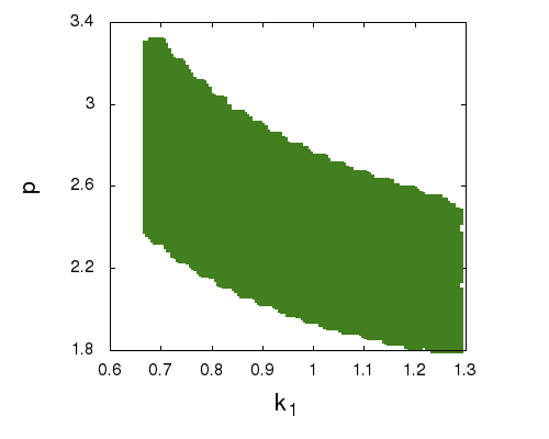
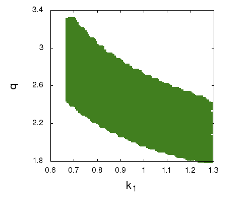
We first consider Category A,B for which the neutrino mass matrix is given in Eqn.(6.3). The parameter ϵitalic-ϵ\epsilon is varied freely to fit the extant data and it is constrained as 0.04<ϵ<0.70.04italic-ϵ0.70.04<\epsilon<0.7. However, to keep the ansatz breaking effect small we restrict the value of ϵitalic-ϵ\epsilon only upto 0.1. For this range of ϵitalic-ϵ\epsilon (0<ϵ<0.10italic-ϵ0.10<\epsilon<0.1) under consideration the parameter spaces are obtained as 1.78<p<3.401.78𝑝3.401.78<p<3.40, 1.76<q<3.421.76𝑞3.421.76<q<3.42 and 0.66<k1<1.30.66subscript𝑘11.30.66<k_{1}<1.3. It is interesting to note a typical feature of this category is that the Dirac CP phase δCPsubscript𝛿𝐶𝑃\delta_{CP} comes out too tiny and thereby generating almost vanishing value of JCPsubscript𝐽𝐶𝑃J_{CP} (106absentsuperscript106\approx 10^{-6}) while the range of the only Majorana phase in this category is obtained as 77o<αM<90osuperscript77𝑜subscript𝛼𝑀superscript90𝑜77^{o}<\alpha_{M}<90^{o}.

Refer to caption
Refer to caption
Figure 1: Plot of p𝑝p vs k1subscript𝑘1k_{1} (left), q𝑞q vs k1subscript𝑘1k_{1} (right) for the Category A,B with ϵ=0.1.italic-ϵ0.1\epsilon=0.1.
Refer to caption
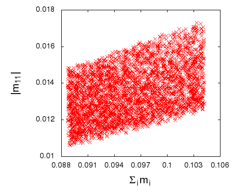
Figure 2: Plot of |m11|subscript𝑚11|m_{11}| vs ΣimisubscriptΣ𝑖subscript𝑚𝑖\Sigma_{i}m_{i} for Category A,B with ϵ=0.1italic-ϵ0.1\epsilon=0.1.

As one of the eigenvalue m3=0subscript𝑚30m_{3}=0 therefore, the hierarchy of the masses is clearly inverted in this category. The sum of the three neutrino masses Σimi(=m1+m2+m3)annotatedsubscriptΣ𝑖subscript𝑚𝑖absentsubscript𝑚1subscript𝑚2subscript𝑚3\Sigma_{i}m_{i}(=m_{1}+m_{2}+m_{3}) and |m11|subscript𝑚11|m_{11}| are obtained as 0.088 eV <Σimi<absentsubscriptΣ𝑖subscript𝑚𝑖absent<\Sigma_{i}m_{i}< 0.104 eV and 0.0102 eV <|m11|<absentsubscript𝑚11absent<|m_{11}|< 0.0181 eV which predict the value of the two quantities below the present experimental upper bounds. To illustrate the nature of variation, in figure 1 we plot p𝑝p vs k1subscript𝑘1k_{1} and q𝑞q vs k1subscript𝑘1k_{1} while in figure 2 a correlation plot of ΣimisubscriptΣ𝑖subscript𝑚𝑖\Sigma_{i}m_{i} with |m11|subscript𝑚11|m_{11}| is shown for ϵ=0.1italic-ϵ0.1\epsilon=0.1 and it is also seen from figure 1 and 2 that the ranges of the parameters do not differ much compare to the values obtained for the whole range of ϵitalic-ϵ\epsilon parameter.

In brief, distinguishable characteristics of this category are i) tiny JCPsubscript𝐽𝐶𝑃J_{CP} and δCPsubscript𝛿𝐶𝑃\delta_{CP} ii) inverted hierarchy of the neutrino masses. At the end of this section we will further discuss the experimental testability of these quantities for all the categories.

6.2.2 Category C

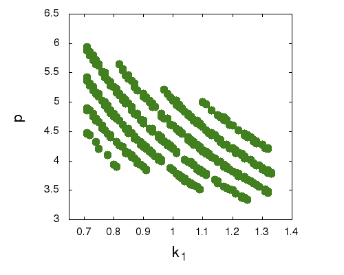
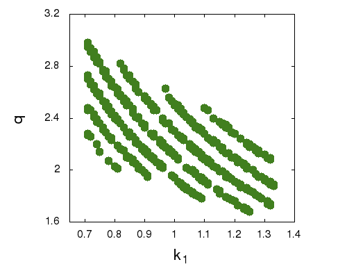
In this case it is found that a small breaking of ϵitalic-ϵ\epsilon (0.02<ϵ<0.090.02italic-ϵ0.090.02<\epsilon<0.09) is sufficient to accommodate all the oscillation data. We explore the parameter space and the ranges obtained as 3.42<p<6.073.42𝑝6.073.42<p<6.07, 1.68<q<3.021.68𝑞3.021.68<q<3.02 and 0.7<k1<1.320.7subscript𝑘11.320.7<k_{1}<1.32. The hierarchy obtained in this case is also inverted due to the vanishing value of m3subscript𝑚3m_{3}.

Refer to caption
Refer to caption
Figure 3: Plot of p𝑝p vs k1subscript𝑘1k_{1} (left), q𝑞q vs k1subscript𝑘1k_{1} (right) for the Category C with ϵ=0.09.italic-ϵ0.09\epsilon=0.09.

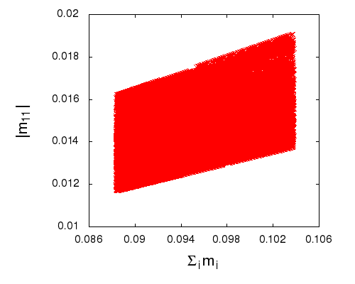
The other two quantities ΣimisubscriptΣ𝑖subscript𝑚𝑖\Sigma_{i}m_{i} and |m11|subscript𝑚11|m_{11}| come out as 0.0118 eV <|m11|<absentsubscript𝑚11absent<|m_{11}|< 0.019 eV and 0.088 eV <Σimi<absentsubscriptΣ𝑖subscript𝑚𝑖absent<\Sigma_{i}m_{i}< 0.105 eV. Similar to the previous category JCPsubscript𝐽𝐶𝑃J_{CP} is vanishingly small due to low value of δCPsubscript𝛿𝐶𝑃\delta_{CP}. The range of the Majorana phase αMsubscript𝛼𝑀\alpha_{M} is obtained as 81o<αM<89osuperscript81𝑜subscript𝛼𝑀superscript89𝑜81^{o}<\alpha_{M}<89^{o}. In figure 3 we plot k1subscript𝑘1k_{1} vs p𝑝p and k1subscript𝑘1k_{1} vs q𝑞q for ϵ=0.09italic-ϵ0.09\epsilon=0.09 that predicts almost the same ranges of the parameters (p𝑝p, q𝑞q and k1subscript𝑘1k_{1}) and all other quantities (|m11|subscript𝑚11|m_{11}|, ΣimisubscriptΣ𝑖subscript𝑚𝑖\Sigma_{i}m_{i}, αMsubscript𝛼𝑀\alpha_{M} and JCPsubscript𝐽𝐶𝑃J_{CP}) as obtained from the whole range of ϵitalic-ϵ\epsilon. We present a correlation plot of ΣimisubscriptΣ𝑖subscript𝑚𝑖\Sigma_{i}m_{i} with |m11|subscript𝑚11|m_{11}| in figure 4.

Refer to caption
Figure 4: Plot of |m11|subscript𝑚11|m_{11}| vs ΣimisubscriptΣ𝑖subscript𝑚𝑖\Sigma_{i}m_{i} for Category C with ϵ=0.09.italic-ϵ0.09\epsilon=0.09.

6.2.3 Category D

In case of Category D, although a priori it is not possible to rule out mνDϵsuperscriptsubscript𝑚𝜈𝐷italic-ϵm_{\nu}^{\prime D\epsilon} without going into the detailed numerical analysis, however in this case even if with ϵ=1italic-ϵ1\epsilon=1 it is not possible to accommodate the neutrino oscillation data. Specifically, the value of θ13subscript𝜃13\theta_{13} is always beyond the reach of the parameter space. Exactly for the same reason the mνsubscript𝑚𝜈m_{\nu} matrix of type A3subscript𝐴3A_{3} in Eqn.(2.5) is phenomenologically ruled out.

6.3 Breaking in Dirac+Majorana sector

In this section we focus on the phenomenology of the neutrino mass matrix where the scaling ansatz is broken in both the sectors. This type of breaking is only relevant for Category A since in this case mDsubscript𝑚𝐷m_{D} is nonsingular after breaking of the ansatz and the resultant mνsubscript𝑚𝜈m_{\nu} gives rise to nonzero θ13subscript𝜃13\theta_{13} along with m30subscript𝑚30m_{3}\neq 0. In all the other categories due to the singular nature of mDsubscript𝑚𝐷m_{D}, inclusion of symmetry breaking in the Majorana sector will not generate m30subscript𝑚30m_{3}\neq 0. Thus we consider only Category A under this scheme.

We consider the breaking in mDsubscript𝑚𝐷m_{D} as mentioned in Eqn.(6.1) and the ansatz broken texture of μ14superscriptsubscript𝜇14\mu_{1}^{4} matrix is given by

μ14superscriptsubscript𝜇14\displaystyle\mu_{1}^{4} =\displaystyle= (r1000k22s3k2(1+ϵ)s30k2(1+ϵ)s3s3)matrixsubscript𝑟1000superscriptsubscript𝑘22subscript𝑠3subscript𝑘21superscriptitalic-ϵsubscript𝑠30subscript𝑘21superscriptitalic-ϵsubscript𝑠3subscript𝑠3\displaystyle\begin{pmatrix}r_{1}&0&0\\ 0&k_{2}^{2}s_{3}&k_{2}(1+\epsilon^{\prime})s_{3}\\ 0&k_{2}(1+\epsilon^{\prime})s_{3}&s_{3}\\ \end{pmatrix} (6.16)

where ϵsuperscriptitalic-ϵ\epsilon^{\prime} is a dimensionless real parameter. The effective neutrino mass matrix mνsubscript𝑚𝜈m_{\nu} comes out as

mνϵAϵ=m0(1k1ppk1pk12(q2eiθ+p2)k1(q2eiθ+p2)pk1(q2eiθ+p2)(q2eiθ+p2))+m0ϵ(00002k12q2eiθk1q2eiθ0k1q2eiθ0)superscriptsubscript𝑚𝜈superscriptitalic-ϵ𝐴italic-ϵsubscript𝑚0matrix1subscript𝑘1𝑝𝑝subscript𝑘1𝑝superscriptsubscript𝑘12superscript𝑞2superscript𝑒𝑖𝜃superscript𝑝2subscript𝑘1superscript𝑞2superscript𝑒𝑖𝜃superscript𝑝2𝑝subscript𝑘1superscript𝑞2superscript𝑒𝑖𝜃superscript𝑝2superscript𝑞2superscript𝑒𝑖𝜃superscript𝑝2subscript𝑚0italic-ϵmatrix00002superscriptsubscript𝑘12superscript𝑞2superscript𝑒𝑖𝜃subscript𝑘1superscript𝑞2superscript𝑒𝑖𝜃0subscript𝑘1superscript𝑞2superscript𝑒𝑖𝜃0\displaystyle m_{\nu\epsilon^{\prime}}^{\prime A\epsilon}=m_{0}\begin{pmatrix}1&k_{1}p&p\\ k_{1}p&k_{1}^{2}(q^{2}e^{i\theta}+p^{2})&k_{1}(q^{2}e^{i\theta}+p^{2})\\ p&k_{1}(q^{2}e^{i\theta}+p^{2})&(q^{2}e^{i\theta}+p^{2})\end{pmatrix}+m_{0}\epsilon\begin{pmatrix}0&0&0\\ 0&2k_{1}^{2}q^{2}e^{i\theta}&k_{1}q^{2}e^{i\theta}\\ 0&k_{1}q^{2}e^{i\theta}&0\\ \end{pmatrix}
+m0ϵ(0k1ppk1p00p00).subscript𝑚0superscriptitalic-ϵmatrix0subscript𝑘1𝑝𝑝subscript𝑘1𝑝00𝑝00\displaystyle+m_{0}\epsilon^{\prime}\begin{pmatrix}0&k_{1}p&p\\ k_{1}p&0&0\\ p&0&0\end{pmatrix}. (6.17)

6.3.1 Numerical results

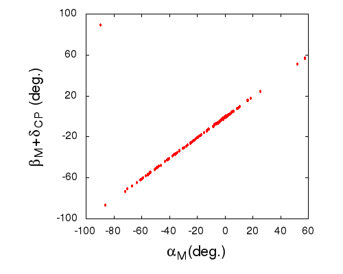
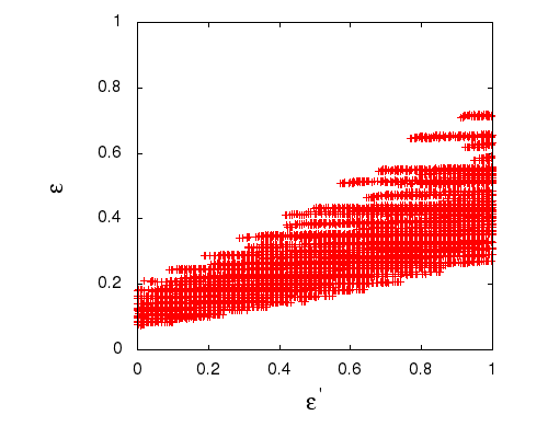
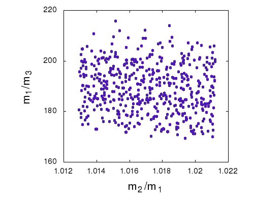
As mentioned above, ϵ=0superscriptitalic-ϵ0\epsilon^{\prime}=0 leads to inverted hierarchy with m3=0subscript𝑚30m_{3}=0 and thus to generate nonzero m3subscript𝑚3m_{3} a small value of ϵsuperscriptitalic-ϵ\epsilon^{\prime} is needed. Similar to the previous cases two breaking parameters ϵitalic-ϵ\epsilon and ϵsuperscriptitalic-ϵ\epsilon^{\prime} can be varied freely through the ranges that are sensitive to the oscillation data and are obtained as 0.06<ϵ<0.680.06italic-ϵ0.680.06<\epsilon<0.68 and 0<ϵ<10superscriptitalic-ϵ10<\epsilon^{\prime}<1. It is to be noted that although the ϵitalic-ϵ\epsilon parameter is restricted due to θ13subscript𝜃13\theta_{13} value, ϵsuperscriptitalic-ϵ\epsilon^{\prime} is almost insensitive to θ13subscript𝜃13\theta_{13} and it can vary within a wide range as 0<ϵ<10superscriptitalic-ϵ10<\epsilon^{\prime}<1. A correlation plot of ϵitalic-ϵ\epsilon with ϵsuperscriptitalic-ϵ\epsilon^{\prime} is shown in figure 5. However, as mentioned earlier, the effect of the breaking term should be smaller than the unbroken one, therefore, to obtain the parameter space for this category we consider breaking of the scaling ansatz in both the sectors only upto 10 % and consequently for all combinatorial values of ϵitalic-ϵ\epsilon and ϵsuperscriptitalic-ϵ\epsilon^{\prime} the parameters p𝑝p, q𝑞q and k1subscript𝑘1k_{1} vary within the ranges as 1.07<p<3.101.07𝑝3.101.07<p<3.10, 1.03<q<3.121.03𝑞3.121.03<q<3.12 and 0.67<k1<1.310.67subscript𝑘11.310.67<k_{1}<1.31. Interestingly, although all the eigenvalues are nonzero in this case, the hierarchy is still inverted. JCPsubscript𝐽𝐶𝑃J_{CP} is found to be tiny (106absentsuperscript106\approx 10^{-6}) again due to small value of δCPsubscript𝛿𝐶𝑃\delta_{CP}. The Majorana phases are obtained as 96o<αM<74osuperscript96𝑜subscript𝛼𝑀superscript74𝑜-96^{o}<\alpha_{M}<74^{o} and 1000<βM+δCP<102osuperscript1000subscript𝛽𝑀subscript𝛿𝐶𝑃superscript102𝑜-100^{0}<\beta_{M}+\delta_{CP}<102^{o} followed by the bounds on ΣimisubscriptΣ𝑖subscript𝑚𝑖\Sigma_{i}m_{i} and |m11|subscript𝑚11|m_{11}| as 0.088 eV <Σimi<absentsubscriptΣ𝑖subscript𝑚𝑖absent<\Sigma_{i}m_{i}< 0.11 eV and 0.010 eV <|m11|<absentsubscript𝑚11absent<|m_{11}|< 0.022 eV which are well below the present experimental upper bounds. In figure 6 we demonstrate the above predictions for ϵ=ϵ=0.1italic-ϵsuperscriptitalic-ϵ0.1\epsilon=\epsilon^{\prime}=0.1. In the left panel of figure 6 the inverted hierarchical nature is shown and in the right panel variation of the Majorana phases is demonstrated.
Refer to caption
Figure 5: Correlated plot of ϵitalic-ϵ\epsilon with ϵsuperscriptitalic-ϵ\epsilon^{\prime}.
Refer to caption
Refer to caption
Figure 6: Plot of (m1/m3)subscript𝑚1subscript𝑚3(m_{1}/m_{3}) vs (m2/m1)subscript𝑚2subscript𝑚1(m_{2}/m_{1}) (left) and βM+δCPsubscript𝛽𝑀subscript𝛿𝐶𝑃\beta_{M}+\delta_{CP} vs αMsubscript𝛼𝑀\alpha_{M} (right) after breaking of the scaling ansatz in both the sectors of Category A for a representative value of ϵ=ϵ=0.1italic-ϵsuperscriptitalic-ϵ0.1\epsilon=\epsilon^{\prime}=0.1.

Some comments are in order regarding predictions of the present scheme:
1. After precise determination of θ13subscript𝜃13\theta_{13} taking full account of reactor neutrino experimental data, it is shown that the hierarchy of the light neutrino masses can be probed through combined utilization of NOν𝜈\nuA and T2K[49] neutrino oscillation experimental results in near future. Thus the speculation of hierarchy in the present scheme will be clearly verified. Moreover, taking the difference of probabilities between P(νμνe)𝑃subscript𝜈𝜇subscript𝜈𝑒P(\nu_{\mu}\rightarrow\nu_{e}) and P(νμ¯νe¯)𝑃¯subscript𝜈𝜇¯subscript𝜈𝑒P(\bar{\nu_{\mu}}\rightarrow\bar{\nu_{e}}) information on the value of JCPsubscript𝐽𝐶𝑃J_{CP} can be obtained using neutrino and anti neutrino beams.
2. More precise estimation of the sum of the three light neutrino masses will be obtained utilizing a combined analysis with PLANCK data[50] and other cosmological and astrophysical experiments[51] such as, Baryon oscillation spectroscopic survey, The Dark energy survey, Large Synoptic Survey Telescope or the Euclid satellite data[52] etc. Such type of analysis will push Σimi0.1similar-tosubscriptΣ𝑖subscript𝑚𝑖0.1\Sigma_{i}m_{i}\sim 0.1 eV (at the 4σ4𝜎4\sigma level for inverted ordering) and Σimi0.05similar-tosubscriptΣ𝑖subscript𝑚𝑖0.05\Sigma_{i}m_{i}\sim 0.05 eV (at the 2σ2𝜎2\sigma level for normal ordering). Thus the prediction of the value of ΣimisubscriptΣ𝑖subscript𝑚𝑖\Sigma_{i}m_{i} in the different categories discussed in the present work will also be tested in the near future. Furthermore, the NEXT-100[53] will probe the value of |m11|subscript𝑚11|m_{11}| up to 0.10.10.1 eV which is a more precise value than the EXO-200[54] experimental range (0.14-0.38 eV).

7 Summary and conclusion

In this work we explore the phenomenology of neutrino mass matrix obtained due to inverse seesaw mechanism adhering i) Scaling ansatz, ii) Texture zeros within the framework of SU(2)L×U(1)Y𝑆𝑈subscript2𝐿𝑈subscript1𝑌SU(2)_{L}\times U(1)_{Y} model with three right handed neutrinos and three left chiral singlet fermions. Throughout our analysis we choose a basis in which the charged lepton mass matrix (mEsubscript𝑚𝐸m_{E}) and the MRSsubscript𝑀𝑅𝑆M_{RS} matrix (appeared in inverse seesaw mechanism due to the coupling of νRsubscript𝜈𝑅\nu_{R} and SLsubscript𝑆𝐿S_{L}) are diagonal. It is found that four is the maximum number of zeros that can be allowed in mDsubscript𝑚𝐷m_{D} and μ𝜇\mu matrices to obtain viable phenomenology. We classify different four zero textures in four different categories depending upon their generic form. Since scaling ansatz invariance always gives rise to θ13=0subscript𝜃130\theta_{13}=0, we have to break such ansatz. We consider breaking in mDsubscript𝑚𝐷m_{D} and also in μ𝜇\mu matrices. We explore the parameter space and it is seen that one category (Category D) is ruled out phenomenologically. The hierarchy obtained in all the cases is inverted and it is interesting to note that all such categories give rise to tiny CP𝐶𝑃CP violation measure JCPsubscript𝐽𝐶𝑃J_{CP} due to small value of δCPsubscript𝛿𝐶𝑃\delta_{CP}. In conclusion, further observation of hierarchy of neutrino masses and CP violation in the leptonic sector in the forthcoming experiments will conclusively refute or admit all these categories obtained in the present scheme.


Acknowledgement
We thank Mainak Chakraborty for discussion and computational help.

References

  • [1] R. N. Mohapatra and J. W. F. Valle, Phys. Rev. D 34, 1642 (1986).
  • [2] J. Bernabeu, A. Santamaria, J. Vidal, A. Mendez and J. W. F. Valle, Phys. Lett. B 187, 303 (1987).
  • [3] R. N. Mohapatra, Phys. Rev. Lett.  56, 561 (1986).
  • [4] J. Schechter and J. W. F. Valle, Phys. Rev. D 25, 774 (1982).
  • [5] A. Palcu, arXiv:1408.6518 [hep-ph].
  • [6] J. Schechter and J. W. F. Valle, Phys. Rev. D 22, 2227 (1980).
  • [7] S. Fraser, E. Ma and O. Popov, Phys. Lett. B 737, 280 (2014) [arXiv:1408.4785 [hep-ph]].
  • [8] H. Hettmansperger, M. Lindner and W. Rodejohann, JHEP 1104, 123 (2011) [arXiv:1102.3432 [hep-ph]].
  • [9] B. Adhikary, A. Ghosal and P. Roy, Indian J. Phys.  88, 979 (2014) [arXiv:1311.6746 [hep-ph]].
  • [10] S. S. C. Law and K. L. McDonald, Phys. Rev. D 87, no. 11, 113003 (2013) [arXiv:1303.4887 [hep-ph]].
  • [11] P. S. B. Dev and A. Pilaftsis, Phys. Rev. D 86, 113001 (2012) [arXiv:1209.4051 [hep-ph]].
  • [12] M. Malinsky, PoS EPS -HEP2009, 288 (2009) [arXiv:0909.1953 [hep-ph]].
  • [13] M. Hirsch, S. Morisi and J. W. F. Valle, Phys. Lett. B 679, 454 (2009) [arXiv:0905.3056 [hep-ph]].
  • [14] D. V. Forero, M. Tortola and J. W. F. Valle, arXiv:1405.7540 [hep-ph].
  • [15] M. C. Gonzalez-Garcia, M. Maltoni, J. Salvado and T. Schwetz, JHEP 1212, 123 (2012) [arXiv:1209.3023 [hep-ph]].
  • [16] D. V. Forero, M. Tortola and J. W. F. Valle, Phys. Rev. D 86 (2012) 073012 [arXiv:1205.4018 [hep-ph]].
  • [17] A. S. Joshipura and W. Rodejohann, Phys. Lett. B 678 (2009) 276 [arXiv:0905.2126 [hep-ph]].
  • [18] R. N. Mohapatra and W. Rodejohann, Phys. Lett. B 644 (2007) 59 [hep-ph/0608111].
  • [19] A. Blum, R. N. Mohapatra and W. Rodejohann, Phys. Rev. D 76, 053003 (2007) [arXiv:0706.3801 [hep-ph]].
  • [20] M. Obara, arXiv:0712.2628 [hep-ph].
  • [21] A. Damanik, M. Satriawan, Muslim and P. Anggraita, arXiv:0705.3290 [hep-ph].
  • [22] S. Goswami and A. Watanabe, Phys. Rev. D 79, 033004 (2009) [arXiv:0807.3438 [hep-ph]].
  • [23] W. Grimus and L. Lavoura, J. Phys. G G 31, 683 (2005) [hep-ph/0410279].
  • [24] M. S. Berger and S. Santana, Phys. Rev. D 74, 113007 (2006) [hep-ph/0609176].
  • [25] S. Goswami, S. Khan and W. Rodejohann, Phys. Lett. B 680 (2009) 255 [arXiv:0905.2739 [hep-ph]].
  • [26] S. Dev, R. R. Gautam and L. Singh, Phys. Rev. D 89, no. 1, 013006 (2014) [arXiv:1309.4219 [hep-ph]].
  • [27] B. Adhikary, M. Chakraborty and A. Ghosal, Phys. Rev. D 86, 013015 (2012) [arXiv:1205.1355 [hep-ph]].
  • [28] P. H. Frampton, S. L. Glashow and D. Marfatia, Phys. Lett. B 536, 79 (2002) [hep-ph/0201008].
  • [29] K. Whisnant, J. Liao and D. Marfatia, AIP Conf. Proc.  1604, 273 (2014).
  • [30] P. O. Ludl and W. Grimus, JHEP 1407, 090 (2014) [arXiv:1406.3546 [hep-ph]].
  • [31] W. Grimus and P. O. Ludl, PoS EPS -HEP2013, 075 (2013) [arXiv:1309.7883 [hep-ph]].
  • [32] J. Liao, D. Marfatia and K. Whisnant, JHEP 1409, 013 (2014) [arXiv:1311.2639 [hep-ph]].
  • [33] H. Fritzsch, Z. z. Xing and S. Zhou, JHEP 1109, 083 (2011) [arXiv:1108.4534 [hep-ph]].
  • [34] A. Merle and W. Rodejohann, Phys. Rev. D 73, 073012 (2006) [hep-ph/0603111].
  • [35] W. Wang, Eur. Phys. J. C 73, 2551 (2013) [arXiv:1306.3556 [hep-ph]].
  • [36] W. Wang, Phys. Lett. B 733, 320 (2014) [Erratum-ibid. B 738, 524 (2014)] [arXiv:1401.3949 [hep-ph]].
  • [37] L. Lavoura, Phys. Lett. B 609, 317 (2005) [hep-ph/0411232].
  • [38] A. Kageyama, S. Kaneko, N. Shimoyama and M. Tanimoto, Phys. Lett. B 538, 96 (2002) [hep-ph/0204291].
  • [39] W. Wang, Phys. Rev. D 90, 033014 (2014) [arXiv:1402.6808 [hep-ph]].
  • [40] G. C. Branco, D. Emmanuel-Costa, M. N. Rebelo and P. Roy, Phys. Rev. D 77 (2008) 053011 [arXiv:0712.0774 [hep-ph]].
  • [41] S. Choubey, W. Rodejohann and P. Roy, Nucl. Phys. B 808, 272 (2009) [Erratum-ibid.  818, 136 (2009)] [arXiv:0807.4289 [hep-ph]].
  • [42] M. Chakraborty, H. Z. Devi and A. Ghosal, Phys. Lett. B 741, 210 (2015) arXiv:1410.3276 [hep-ph].
  • [43] B. Adhikary, A. Ghosal and P. Roy, JHEP 0910 (2009) 040 [arXiv:0908.2686 [hep-ph]].
  • [44] B. Adhikary, A. Ghosal and P. Roy, JCAP 1101 (2011) 025 [arXiv:1009.2635 [hep-ph]].
  • [45] B. Adhikary, A. Ghosal and P. Roy, Mod. Phys. Lett. A 26 (2011) 2427 [arXiv:1103.0665 [hep-ph]].
  • [46] W. Grimus, A. S. Joshipura, L. Lavoura and M. Tanimoto, Eur. Phys. J. C 36, 227 (2004) [hep-ph/0405016].
  • [47] B. Adhikary, M. Chakraborty and A. Ghosal, JHEP 1310, 043 (2013) [Erratum-ibid.  1409, 180 (2014)] [arXiv:1307.0988 [hep-ph]].
  • [48] J. Beringer et al. [Particle Data Group Collaboration], Phys. Rev. D 86, 010001 (2012).
  • [49] K. Ieki, T2K-THESIS-040.
  • [50] P. A. R. Ade et al. [Planck Collaboration], Astron. Astrophys.  571, A16 (2014) [arXiv:1303.5076 [astro-ph.CO]].
  • [51] J. Lesgourgues and S. Pastor, New J. Phys.  16, 065002 (2014) [arXiv:1404.1740 [hep-ph]].
  • [52] Audren B, Lesgourgues J, Bird S, Haehnelt M G and Viel M 2013 J. Cosmol. Astropart. Phys. JCAP01(2013)026
  • [53] D. Lorca [ David Lorca for the NEXT Collaboration], arXiv:1411.0475 [physics.ins-det].
  • [54] M. Auger et al. [EXO Collaboration], Phys. Rev. Lett.  109, 032505 (2012) [arXiv:1205.5608 [hep-ex]].