Six–vertex model with domain wall boundary conditions in the Bethe–Peierls approximation

Abstract

We use the Bethe–Peierls method combined with the belief propagation algorithm to study the arctic curves in the six vertex model on a square lattice with domain-wall boundary conditions, and the six vertex model on a rectangular lattice with partial domain-wall boundary conditions. We show that this rather simple approximation yields results that are remarkably close to the exact ones when these are known, and allows one to estimate the location of the phase boundaries with relative little effort in cases in which exact results are not available.

1 Introduction

Usually, boundary conditions have no effect on the equilibrium properties of statistical models in the thermodynamic limit. Still, boundary conditions may affect the equilibrium behaviour of strongly constrained models and, in particular, they may impose the macroscopic separation of phases. In such cases, the boundary between an internal spatial region, in which the configuration is typical of equilibrium with the bulk parameters, and an external spatial region, frozen by the boundary conditions is named the arctic curve. The external region is called arctic (for frozen) and the internal region is called temperate (for fluctuating). The arctic curve first appeared in the study of domino tilings of Aztec diamonds [1, 2, 3, 4], then in lozenge tilings of large hexagons [5, 6], and later in more general dimer [7] and vertex models [3, 4, 8, 9, 10, 11, 12]. In these systems phase separation exists for a wide choice of fixed boundary conditions.

The six vertex model was first introduced to model ferroelectricity [13, 14, 15, 16, 17], and it has links with the models mentioned above. It is commonly defined on a square lattice with $N\times N$ vertices. (We will consider here the extension to rectangular systems with $N\times M$ vertices as well.) Arrows are placed along the links, with two possible orientations for each. The six vertex rule imposes that two arrows should point in and two should point out of each vertex. Energies and, consequently, statistical weights are assigned to each vertex. If complete arrow reversal symmetry is assumed, three parameters, $a$, $b$, $c$, characterise these weights, with the two first ones associated to local ferroelectric order and the last one linked to antiferroelectric order (see Fig. 1).

The solution to the most general six vertex model with periodic boundary conditions, in the form of its bulk free-energy density, was given by Sutherland [18] who extended Lieb’s treatment with the Bethe Ansatz technique to generic values of the vertex weights. The value taken by the following parameter (see Fig. 1)

$$\Delta=\frac{a^{2}+b^{2}-c^{2}}{2ab}$$ (1.1)

distinguishes the three phases of the model: for $\Delta>1$ the equilibrium state has ferroelectric (FE) order, for $\Delta<-1$ it has antiferroelectric (AF) order, and for $|\Delta|<1$ it is disordered (D). The D-FE phase transition is first-order while the D-AF transition is characterized by an essential singularity reminiscent of the Kosterlitz-Thouless type.

The six vertex model with domain wall boundary conditions was introduced in [19] to study correlation functions in exactly solvable models [20]. In a few words, domain-wall boundary conditions correspond to all arrows on the bottom and top boundaries being incoming while all arrows on the left and right boundaries being outgoing, see Fig. 2 (or vice versa). More recently, the interest in this model has been pushed by its connection with algebraic combinatorics and the enumeration of alternating sign matrices. The partition function satisfies a recurrence relation [21, 19], that leads to a determinant formula [21], exploited by Korepin and P. Zinn-Justin (see also [22]) to derive exact expressions for the free-energy densities in the disordered and ferroelectric phases [23]. The antiferroelectric free-energy density was obtained in [24] by using a matrix model representation of the determinant. Although the phase diagram remains unaltered, and still given by the case with $|\Delta|=1$, the free-energy densities in the disordered and antiferromagnetic phases, are different from the ones found with periodic boundary conditions, even in the thermodynamic limit. Curiously enough, the free-energies take much simpler expressions as functions of the parameters $a,b,c$ under the domain-wall boundary conditions. The D-FE transition becomes continuous while the D-AF remains of infinite order.

The six vertex model can be mapped onto the problem of domino tilings on Aztec diamonds [17, 16] for a particular choice of vertex weights [19] and, in consequence, it also admits an arctic curve separating an external finite density boundary with ferroelectric order from an internal region that is either disordered or antiferroelectrically ordered for $|\Delta|<1$ or $\Delta<-1$, respectively. On the free-fermion point ($\Delta=0$) with $a=b$ the arctic curve is a circle [3, 4]. On the less restrictive free-fermion cases with $a\neq b$ the arctic curves are ellipses [8]. Numerical evidence for the existence of an arctic curve for general values of the parameters was presented in [25, 26]. Various analytic, though not yet proven to be exact (except for $\Delta=0$ where the derivation is rigorous), methods have been employed to determine the arctic curves in the disordered phase with $\Delta\neq 0$ [9, 10] and even in the antiferroelectric phase [11].

As mentioned above, very powerful and interesting analytic methods allow one to understand the statics of the six vertex model, and the phase separation induced by special boundary conditions. A summary of modern methods applied to this problem can be found in [27] and a review on arctic curves in the six vertex model is given in [12]. Still, as soon as one lifts the integrability conditions satisfied by the six (and eight) vertex model, these techniques are no longer useful. Approximate methods, such as the Bethe–Peierls approximation [28] and its modern versions, like the cavity method and the belief propagation algorithm [29, 30, 31, 32], can then be of great help to obtain the phaser diagram and equilibrium properties of generic vertex models. This method was applied in [33, 34] to analyse the sixteen vertex model with parameters close to the ones of artificial spin-ice samples [35, 36]. Surprisingly enough, the method gave very accurate, sometimes even exact, results when applied to the integrable six and eight vertex cases. Moreover, cluster generalizations have been used to obtain phase diagrams and thermodynamical properties of vertex models with a much larger state space [37, 38, 39, 40, 41, 42], both in two and three dimensions.

The work in [33, 34] concerned homogeneous systems (except for distinguishing between two different sublattices, when necessary) with periodic boundary conditions. Here we aim at extending this work to inhomogeneous systems, making it possible to describe the phase separation phenomenon induced by domain–wall boundary conditions. This will imply an increase in the computational complexity by a factor $N\times M$ which, even in the large $N$ and $M$ limit, can be dealt with thanks to the belief propagation (BP) algorithm, which is particularly efficient at finding minima of a Bethe–Peierls free-energy even in inhomogeneous systems. As an example of results that we obtain in this work, for which there are no rigourous predictions, there is the behavior of the interface separating the disordered region from the AF phase in the case of parameters corresponding to the AF bulk phase.

We end this introductory section by stating that domain wall boundary conditions could be easily imposed experimentally in artificial spin-ice samples [35, 36]. A possible way to do this would be to fabricate an array where the edge islands are different in some way (larger, or from a different magnetic material) in order to make them more stable. Modern visualization experimental methods [43, 44, 45, 46] should then allow one to see the phase separating curves in the lab.

The paper is organised as follows. In Sec. 2 we recall the definition of the six vertex model and the properties that are of interest to our work. Section 3 is devoted to a short description of the belief propagation method as applied to the six vertex model with domain wall boundary conditions. In Sec. 4 we present our results. In Sec. 5 we discuss several lines for future work.

2 The six vertex model and its arctic curve

2.1 Definition, phases and free-energies

The six vertices defining the model together with their statistical weights are shown in Fig. 1.

Figure 1: The six vertices in the six vertex model and their Boltzmann weights, $\omega_{1},\dots,\omega_{6}$.

An alternative parametrisation of the Boltzmann weights is

$$a=\sin(\lambda+\eta)\qquad\;\;\;b=\sin(\lambda-\eta)\qquad\;\;\;c=\sin 2\eta$$ (2.1)

with $\lambda$ the ‘rapidity’ variable and $\eta$ the ‘crossing’ parameter. The parameter $\Delta=\cos 2\eta$ serves to locate the phase transitions.

In the disordered (D) phase $|\Delta|=|\cos 2\eta|<1$ and the parameters $\lambda$ and $\eta$ are constrained to $\eta\leq\lambda\leq\pi-\eta$ and $0<\eta<\pi/2$. In the free-fermion case $\Delta=0$ and $\eta=\pi/4$. In the free-fermion and symmetric $a=b$ case, $\Delta=0$, $\eta=\pi/4$ and $\lambda=\pi/2$. In the spin-ice case $a=b=c$ implies $\Delta=1/2$, $\eta=\pi/6$ and $\lambda=\pi/2$.

Let us first focus on the square lattice model. The domain-wall boundary conditions (DWBC) are sketched in Fig. 2. The free-energy density per site in the disordered phase with these boundary conditions is [19, 23]

$$f^{D}_{DW}=-\ln\left(\frac{\alpha\sin(\lambda+\eta)\sin(\lambda-\eta)}{\sin[\alpha(\lambda-\eta)]}\right)\qquad\mbox{with}\qquad\alpha=\frac{\pi}{\pi-2\eta}\;.$$ (2.2)

When compared to the (much more involved) expression for periodic boundary conditions [18] one finds $f^{D}_{DW}>f^{D}_{P}$. The extension of this analysis to the antiferroelectric (AF) and ferroelectric (FE) phases shows that $f^{AF}_{DW}>f^{AF}_{P}$ in the AF phase [24] while $f^{FE}_{DW}=f^{FE}_{P}$ in the FE one [19, 23]. The macroscopic phase separation is intimately linked to the difference between the free-energies for different boundary conditions. The D-FE phase transition is continuous and the D-AF transition is of infinite order under DWBC.

Figure 2: An example of domain wall boundary conditions.

2.2 The arctic curve

The arctic curve(s) delimiting the spatial regions with different ordering properties is (are) defined in the scaling limit in which the number of lines in each direction, $N$ on a $NxN$ square lattice, tends to infinity while the lattice spacing, $\delta$, vanishes keeping the two linear size of the lattice fixed.

In the case in which the bulk parameters select a disordered state, the phase separation induces five spatial regions in the sample: four external ferroelectric ones, close to the four corners and an internal one, that is the disordered region $D$.

In the case in which the bulk parameters select the AF state, the phase separation occurs in two steps, in the sense that an intermediate disordered spatial region separates the external FE region fixed by the boundaries, and the internal AF region fixed by the bulk parameters. There is therefore one arctic curve and one temperate (between D and AF regions) curve in this problem.

Some analytic expressions for the interface between frozen and temperate regions in the six vertex model on a square lattice are known and we summarise them below.

2.2.1 Boundary between the FE and the D phase.

Colomo and Pronko used boundary correlation functions to get a closed expression for the coordinates of the contact points between the arctic curve and the system’s boundaries [10]

$$\kappa=\frac{\alpha\cot[\alpha(\lambda-\eta)]-\cot(\lambda+\eta)}{\cot(\lambda-\eta)-\cot(\lambda+\eta)}$$ (2.3)

for generic $|\Delta|<1$. In particular, for $\lambda=\pi/2$ one finds $\kappa=1/2$ for all $\eta$.

The form of the arctic curve linking these points is highly non-trivial and for generic $\eta$ non-algebraic. Some special cases have been known for more than a decade.

Jockusch et al [4] proved the arctic circle theorem for the free-fermion case $\Delta=0$ with $a=b$ in which the arctic curve is just a circle,

$$\left(x-\frac{1}{2}\right)^{2}+\left(y-\frac{1}{2}\right)^{2}=\frac{1}{4}\;.$$ (2.4)

In the free fermion case, $\Delta=0$ and $\eta=\pi/4$, the arctic curve can be computed exactly for $a\neq b$ and it is an ellipse tangent to the four sides of the square

$$(1+t^{2})(x+y-1)^{2}+t^{2}(1+t^{2})(x-y)^{2}=t^{2}$$ (2.5)

with

$$t=\frac{b}{a}=\tanh\left(\lambda-\frac{\pi}{4}\right)\;.$$ (2.6)

For $t=1$ one recovers the article circle.

With the emptiness correlation function, and a conjecture on its behavior, Colomo and Pronko obtained an implicit expression for the arctic curve in the general $\Delta\neq 0$ case [9, 10, 47]. In section 6.3 in [10], eqs. (6.17)-(6.19) present a parametric representation of this curve. In general, the curve is a transcendental function. For special values of $\Delta$, that correspond to what are called the roots-of-unity in the quantum group context, the curve becomes algebraic [10, 12]. In particular, at the spin-ice point ($a=b=c$ and $\Delta=1/2$) the arctic curve is given by the portion of the ellipse

$$(x+y-2)^{2}+3(x-y)^{2}-3=0$$ (2.7)

in which $x,y\in[0,1/2]$. The contact points in the lower left quadrant are $(1/2,0)$ and $(0,1/2)$, in other words, $\kappa=1/2$.

2.2.2 Boundary between the FE and AF phases.

Colomo, Pronko and Zinn-Justin [11] used the emptiness correlation function method to estimate the arctic curve between the external frozen region and an intermediate disordered region that separates it from the bulk with AF order. As far as we know, there is no prediction for the internal boundary between the D and AF regions.

3 Method

In this section we introduce the key ideas and equations of the belief propagation (BP) algorithm, which are needed to apply the method to the present problem.

We label the lattice edges $i,j,k,\ldots$ and the vertices $a,b,c,\ldots$ (not to be confused with the vertex weight parameters used above). If an edge $i$ is incident on a vertex $a$ we say that the edge belongs to the vertex and we write $i\in a$. In the language of probabilistic graphical models (see e.g. [31] and refs. therein for the relationship between these models and statistical mechanics), edges (respectively, vertices) are variable nodes (resp. factor nodes) in a factor graph. In this notation the full Boltzmann weight can be written as

$$\psi=\prod_{a}\psi_{a}(s_{a}),$$ (3.1)

where $s_{a}=\{s_{i},i\in a\}$ and $s_{i}$ represents the orientation of edge $i$, say, positive towards the right (up) for horizontal (vertical) links, as in [25].

The BP algorithm is a message–passing algorithm for finding the minima of an approximate (mean–field–like) variational free-energy (a generalization of the Bethe–Peierls one) which can be obtained by truncating the cumulant expansion of the entropy of the model, by keeping only edge and vertex contributions or, in other words, the free-energy of the cluster variational method (see [31] for a recent review) with vertices as maximal clusters:

$${\cal F} = \sum_{a}\sum_{s_{a}}H_{a}(s_{a})p_{a}(s_{a})+$$ (3.2)

$$+k_{B}T\left[\sum_{a}\sum_{s_{a}}p_{a}(s_{a})\ln p_{a}(s_{a})-\sum_{i}\sum_{s_{i}}p_{i}(s_{i})\ln p_{i}(s_{i})\right],$$

where $H_{a}(s_{a})=-k_{B}T\ln\psi_{a}(s_{a})$ is the contribution of vertex $a$ to the model Hamiltonian and $p_{a}(s_{a})$ (respectively $p_{i}(s_{i})$) is the probability distribution of vertex $a$ (resp. edge $i$). The above variational free-energy has to be minimized with respect to the vertex and edge probability distributions, subject to the constraints of normalization

$$\sum_{s_{a}}p_{a}(s_{a})=1,\quad\forall a\qquad\sum_{s_{i}}p_{i}(s_{i})=1,\quad\forall i$$ (3.3)

and marginalization

$$\sum_{s_{a\setminus i}}p_{a}(s_{a})=p_{i}(s_{i}),\quad\forall a,\quad\forall i\in a,$$ (3.4)

where $s_{a\setminus i}=\{s_{j},j\in a,j\neq i\}$.

Minima of the variational free-energy correspond [30, 31] to fixed points of the BP algorithm. In the latter picture, a vertex $a$ sends a message $m_{a\to i}(s_{i})$ to an edge $i\in a$, which depends on the edge orientation. Up to a normalization constant, the edge and vertex probability distributions can be written as functions of the messages as

$$p_{i}(s_{i})\propto\prod_{a\ni i}m_{a\to i}(s_{i}),\qquad\qquad p_{a}(s_{a})\propto\psi_{a}(s_{a})\prod_{i\in a}\prod_{b\ni i}^{b\neq a}m_{b\to i}(s_{i}).$$ (3.5)

Rewriting the marginalization condition Eq. (3.4) in terms of messages one obtains, again up to a normalization constant,

$$m_{a\to i}(s_{i})\propto\sum_{s_{a\setminus i}}\psi_{a}(s_{a})\prod_{j\in a}^{j\neq i}\prod_{b\ni j}^{b\neq a}m_{b\to j}(s_{j}),$$ (3.6)

the main iterative equation of the BP algorithm, the fixed point of which gives the message values at equilibrium, to be used in the computation of the edge and vertex probability distributions, Eq. (3.5), and of the free-energy, Eq. (3.2). In the following we shall often refer to the free-energy density $f={\cal F}/(NM)$.

Domain–wall boundary conditions are easily represented in this scheme, by introducing boundary messages, sent by auxiliary vertices to boundary edges which vanish if and only if the edge orientation differs from the one imposed by the boundary conditions. In more detail, what we mean by this is the following. Consider a boundary edge $i$ and assume that it is horizontal, on the right boundary of the lattice. This edge belongs to a single vertex $a$, which sits on its left side. Introduce the auxiliary vertex $b$, sitting on the right of the edge $i$. Since the polarization of $i$ is constrained to be rightward ($+1$ in our representation), we set $m_{b\to i}(-1)=0$.

4 Results

In this Section we present the results that we obtained by using the BP algorithm explained in Sec. 3.

4.1 Square lattice

We first study the model on a square lattice for which analytic expressions for the interfaces are known.

4.1.1 The free-energy.

In [33] the Bethe-Peierls approximation was used to study the equilibrium properties of the sixteen and, in particular, the six vertex model with periodic boundary conditions. Defining the six vertex model on a tree, the exact FE free-energy density was found, while in the D and AF phases very good approximations to the exact expressions, that get better and better far from the transition, were derived. Although the free-energy densities obtained with the Bethe-Peierls approximation in the infinite size limit (that in the homogeneous case can be treated analytically) are not exact, the location of the different transition lines (between D and FE, and D and AF, phases) are.

First, we check that the BP free-energy densities of the six-vertex model with DWBC satisfies $f_{DW}>f_{P}$ for a square lattice system. In Fig. 3 we show the approach to the thermodynamic limit of the free-energy density at the spin-ice point $a=b=c=1$ ($\Delta=1/2$). The numerical data are fitted with the form

$$f_{DW}^{D}(N)\simeq f_{DW}^{D}(N\to\infty)+cN^{-\psi}\;.$$ (4.1)

We find $\psi\simeq 1.6-1.7$ and $f_{DW}^{D}(N\to\infty)\simeq-0.246$. The estimate for the free-energy density in the thermodynamic limit is larger than the one for periodic boundary conditions, $f_{P}^{D}=-\ln(3/2)\simeq-0.404$, that is Pauling’s result also found on the tree. We note that the free-energy-density for domain-wall boundary conditions on the tree is slightly larger than the exact result, $f_{DW}^{D}=-\ln(3\sqrt{3}/4)\simeq-0.262$ [23]. The fact that the BP approximation slightly over-estimates the free-energy (with respect to the exact result) was also found for periodic boundary conditions [33].

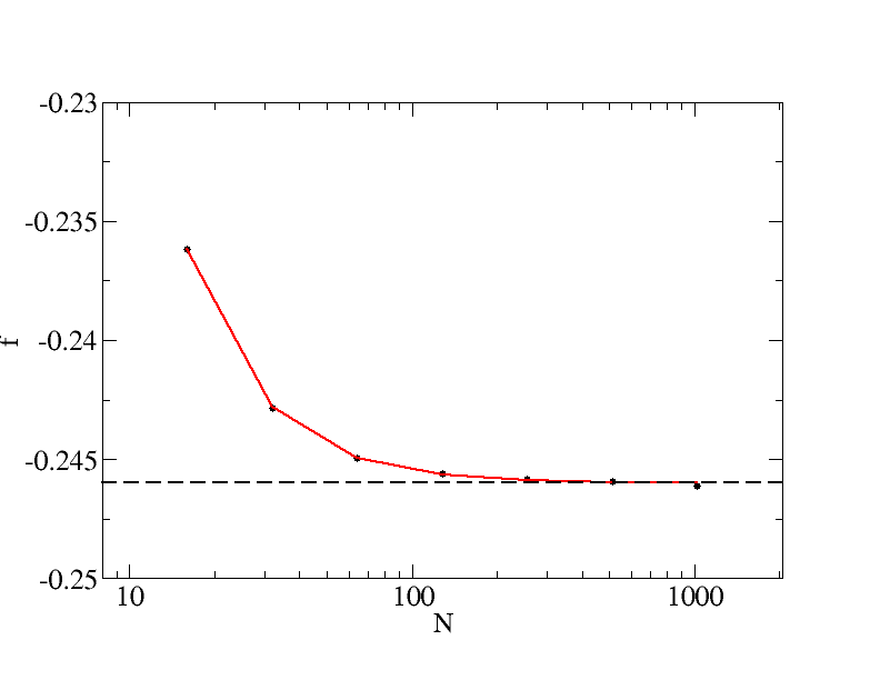
Figure 3: BP free-energy density vs. lattice size $N$ for the six vertex model on a square lattice with domain-wall boundary conditions at the spin–ice point, $a=b=c=1$ (data points joined by straight lines). The asymptotic estimate, $f_{DW}^{D}\simeq-0.246$, is shown with a dotted horizontal lines. The exact value, $f^{D}_{DW}\simeq-0.262$, lies beyond the vertical range of variation of this graph.

In Fig. 4 we compare our free-energy density with the exact one [23], in the D and FE phases. In particular we consider a square lattice with $N=32$, we set $b=c=1$ and vary $a$ in the range $[1,3]$. Notice that $a=1$ corresponds to the spin–ice point $\Delta=1/2$, while at $a=2$ ($\Delta=1$) the system is expected to undergo (in the thermodynamical limit) a continuous phase transition between the D and FE phases. Our finite size analysis shows instead a continuous variation from a D bulk behaviour for $a<2$ to an FE bulk behaviour for $a>2$. In agreement with data reported in Fig. 3, the corrections to our free-energy density that we obtain upon increasing $N$ from 32 to 1000 are of order $10^{-3}$, hence not resolvable on the scale of Fig. 4.

The exact FE free-energy of the two-dimensional model in the $N\to\infty$ limit is $f^{FE}_{DW}=f^{FE}_{P}=-\ln a$ and it is shown with a blue line in Fig. 4. The BP algorithm should also give this result in the infinite size limit. We ascribe the deviation from of the black curve in Fig. 4 from the asymptotic limit to finite size effects.

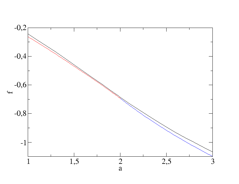
Figure 4: Free-energy density vs. $a$ for the six vertex model on a square lattice with parameters $b=c=1$ and under domain-wall boundary conditions. The BP data for a system with linear size $N=32$ (black line) should be compared to the exact result [23] in the thermodynamical limit (red line: D phase, blue line: FE phase).

A similar analysis is shown in Fig. 5 in the D and AF phases (for the exact free-energy density in the AF phase see [24]). We set $N=32$, $a=b=1$ and vary $c$ in the range $[1,3]$. Again $c=1$ corresponds to the spin–ice point $\Delta=1/2$, while at $c=2$ ($\Delta=-1$) the system is expected to undergo (in the thermodynamical limit) a continuous phase transition between the D and AF phases. Here our finite size results show a reminiscence of the infinite size phase transition. For $c\in[2.08,2.13]$ we find both a (stable) AF phase and a (metastable) D phase (the difference in free-energy density between these two phases is $\sim 10^{-4}$, not resolvable on the scale of Fig. 5), while for $c<2.08$ we have only the D phase and for $c>2.13$ only the AF phase is found. This allows us to locate a finite size phase transition at $c\simeq 2.08$. Upon increasing $N$ the transition point seems to tend towards $c=2$, but it is hard to prove that the transition line is captured exactly as $N\to\infty$.

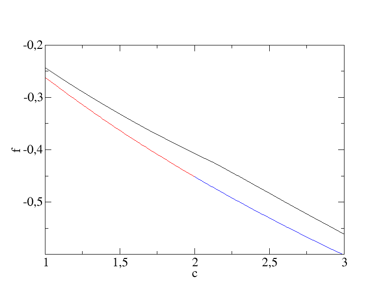
Figure 5: Free-energy density vs. $c$ for the six vertex model on a square lattice with parameters $a=b=1$ and under domain-wall boundary conditions. The BP data for a system with linear size $N=32$ (black line) should be compared to the exact result [23, 24] in the thermodynamical limit (red line: D phase, blue line: AF phase).

4.1.2 Arctic circle.

We work out the case $\Delta=0$ and $a=b$ in which the arctic curve should be a circle. In Fig. 6 we plot the polarization $\langle s_{i}\rangle$ of the horizontal edges for a $1024\times 1024$ lattice, with (following the convention introduced in Sec. 3 above) $s_{i}=+1$ (respectively, $-1$) for a rightward (resp. leftward) edge. The exactly known arctic circle is drawn as a white solid line. The agreement is remarkable, considering that we are applying a mean–field like technique to a system in its critical state. The temperate region is slightly overestimated by the BP approximation, though this might be just a finite size effect. This is better observed in Fig. 7, where we plot the polarization (from now on, the polarization of the horizontal edge at position $(x,y)$ will be denoted by $p_{x}(x,y)$) of the horizontal edges at a fixed vertical coordinate $y=1/8$, for different lattice sizes, together with the left intersection of the exact arctic circle with $y=1/8$.

Figure 6: BP polarization of the horizontal edges for the free-fermion case, $\Delta=0$, with $a=b$, on a square lattice with $1024\times 1024$ lattice vertices. The white line is the exact arctic circle.

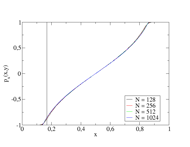
Figure 7: BP polarization of the horizontal edges for the free-fermion case, $\Delta=0$, with $a=b$, for $y=1/8$ and different system sizes $N$. The vertical line denotes the left intersection of the exact arctic circle with $y=1/8$.

Given that the system is critical, we expect simple power–laws for the scaling of its observables. We denote by $x_{0}(y)$ the (exactly known) arctic curve. Observing that in the frozen regions on the right of Fig. 6 the polarization $p_{x}(x,y)$ tends to 1, we have considered the deviation $1-p_{x}(x,y)$ as a function of $N^{\alpha}(x-x_{0}(y))$ for fixed $y$ and $x>1/2$ and looked for data collapse. The best results have been obtained with $\alpha\simeq 1/6$ and the corresponding plot is reported in Fig. 8, with the vertical axis both in linear (left panel) and log (right panel) scale. A good collapse is obtained for $x\gtrsim x_{0}(y)$ suggesting that our estimate of the arctic curve is very close to the exact one and that the scaling law holds in the frozen phase only.

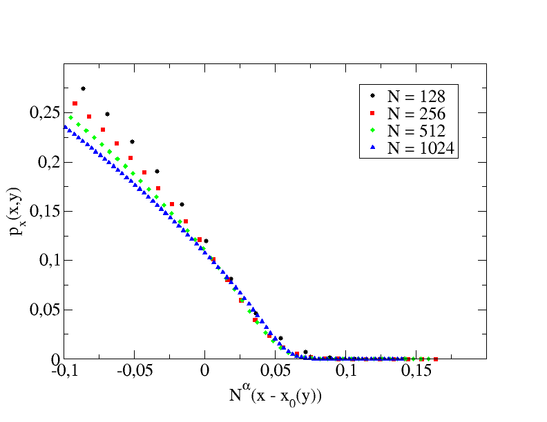
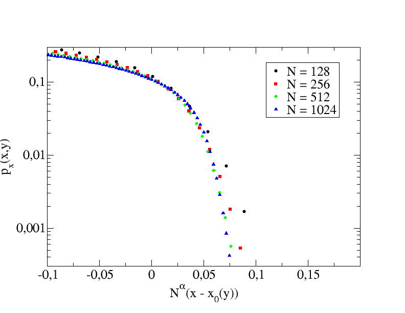
Figure 8: BP polarization (deviation from the value in the frozen phase) of the horizontal edges vs. $N^{\alpha}(x-x_{0}(y))$ for the free-fermion case, $\Delta=0$, with $a=b$, for $y=3/4$, $\alpha=1/6$ and different system sizes $N$. Vertical axis in linear (left panel) and log (right panel) scale.

4.1.3 Arctic ellipses.

We now work out the case $\Delta=1/2$ and $a=b=c$ in which the arctic curve should be an ellipse. In Fig. 9 we plot, as in the previous subsection, the polarization of the horizontal edges and the exactly known arctic ellipse. The agreement is still remarkable. Our numerical data are consistent with the exact $\kappa=1/2$ values for the contact points. However, also in this case the temperate region seems slightly overestimated by the BP approximation. Indeed, in Fig. 10. we display the polarisation of the horizontal edges as a function of the horizontal coordinate for a cut at constant vertical coordinate, $y=1/8$. The right panel shows a zoom close to the $x$ value where the exact article curve lies. One sees that the finite $N$ curves obtained with the BP algorithm suggest a location of the sharp boundary at a value of $x$ that will be closer to the edge of the system than the exact one.

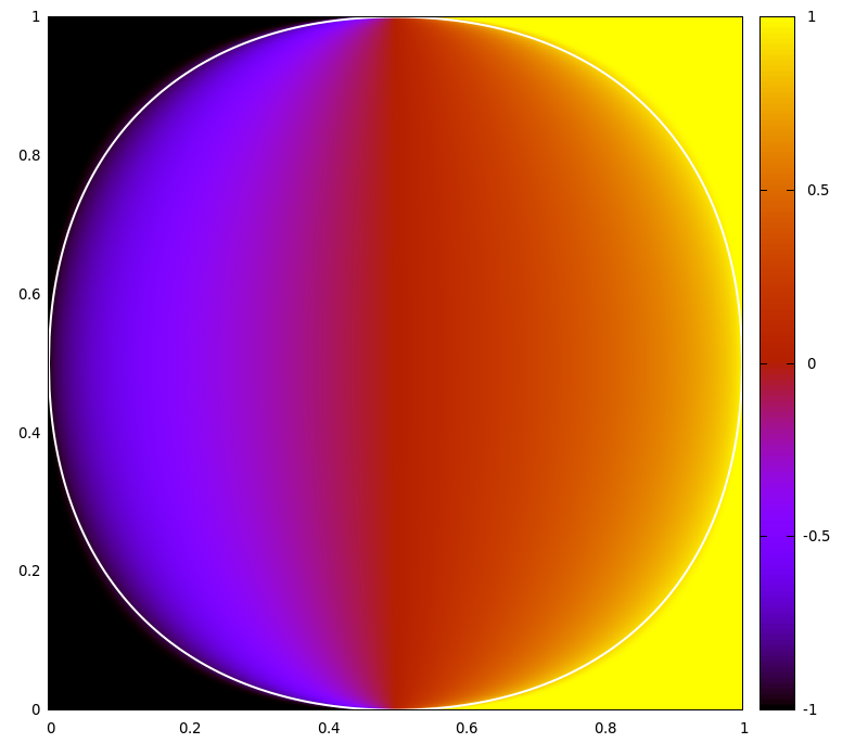
Figure 9: BP polarization of the horizontal edges at the spin–ice point, $a=b=c$, $\Delta=1/2$.

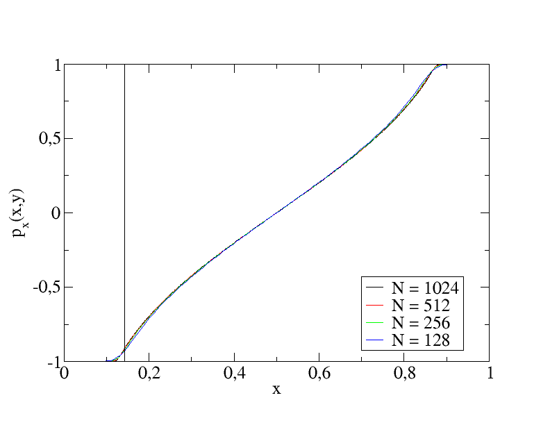
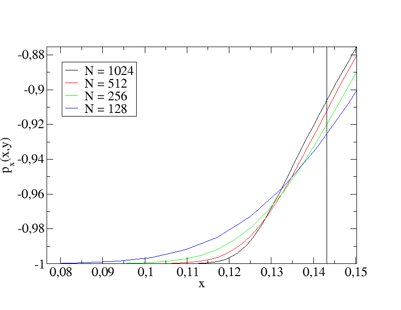
Figure 10: Left panel: BP polarization of the horizontal edges at the spin–ice point, $a=b=c$, $\Delta=1/2$, for $y=1/8$ and different system sizes $N$. The vertical line denotes the left intersection of the exact arctic ellipse with $y=1/8$. Right panel: magnification close to the arctic ellipse.

4.1.4 Double interfaces in the AF phase.

For bulk parameters such that the system is in the AF phase, the domain wall boundary conditions impose a frozen external region, an intermediate disordered ‘buffer’ and an internal region with AF order. This is shown in Fig. 11 for different values of $c>2$ and $a=b=1$ (the phase transition between the bulk D and AF phases is located at $c=2$).

The shrinking of the internal AF region as $c$ decreases towards 2 suggests a continuous transition: indeed, this transition is known to be continuous, and in particular of infinite order [24] (a feature which of course cannot be reproduced by our mean–field–like approach).

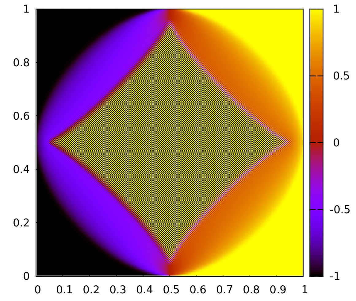
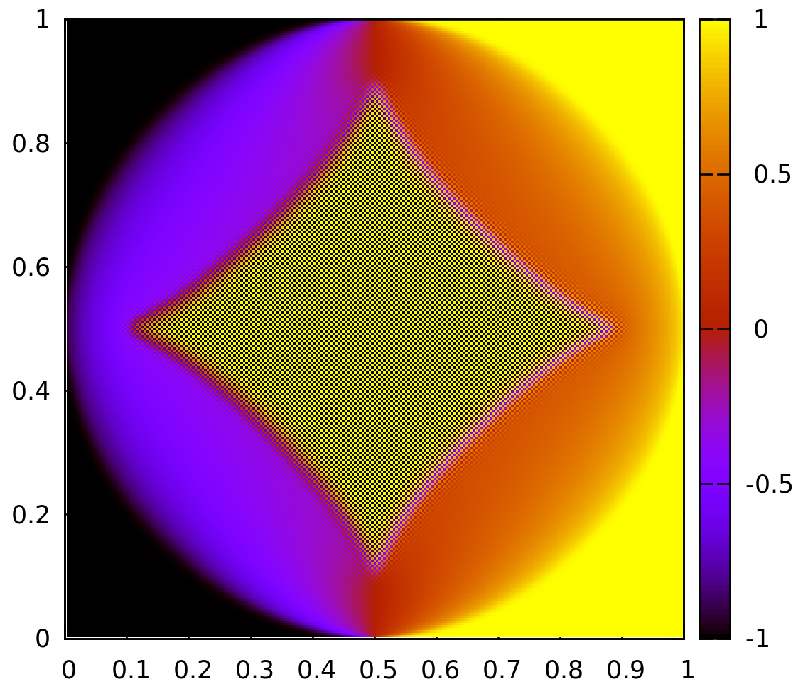
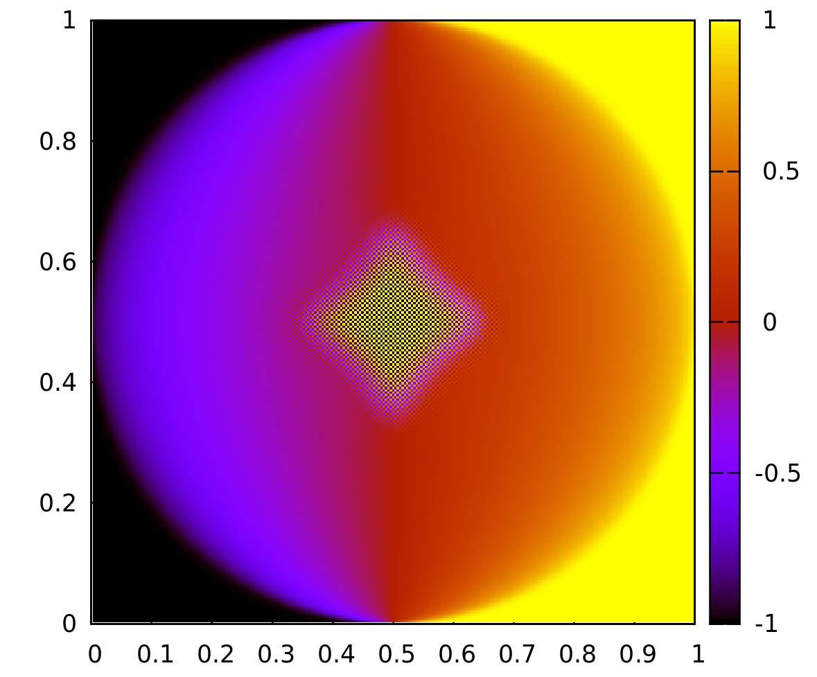
Figure 11: BP polarization of the horizontal edges for $\Delta<-1$ with $a=b=1$ and $c=3,2.5,2.05$ from left to right. The system size is $N=256$.

While the variation of the AF–D boundary with $c$ is evident from Fig. 11, it is not the same for the D–frozen boundary (the arctic curve). We can however understand its trend from Fig. 12, where we have plotted the polarization of the horizontal edges at a fixed height $y=1/8$ for various values of $c$. Looking at the points where the polarization saturates it is now evident that the arctic curve gets larger as $c$ decreases, both for $c>2$ (bulk AF phase, curves characterized by oscillations in the center) and for $c<2$ (bulk D phase, smooth curves).

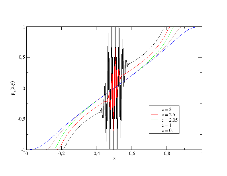
Figure 12: BP polarization of the horizontal edges at $a=b=1$ meaning $\Delta=(2-c^{2})/2$, system size $N=256$, and $y=1/8$, for different $c$ values. For $c=3,\ 2.5,\ 2.05$, $\Delta<-1$ and the system prefers the AF configuration in the bulk. For $c=1,\ 0.1$, $0<\Delta<1$ and the system prefers the D configuration in the bulk.

4.2 Rectangular systems with partial domain wall boundary conditions

In the framework of the BP algorithm it is straightforward to consider rectangular lattices and different types of boundary conditions. In order to illustrate this, in the present Section we discuss the six vertex model on rectangular lattices, with partial domain wall boundary conditions (pDWBC). These are a generalization of DWBC to rectangular systems [48, 49]. Consider a rectangular lattice with $N\times M$ vertices (in the following we shall assume $N>M$ to fix ideas) and impose DWBC–like boundary conditions on three sides of the lattice, leaving the $4^{\rm th}$ side free. Following the convention we have set up in Fig. 2 we will have inward–pointing edges on the bottom side and outward–pointing edges on the left and right sides. The ice rule then implies that on the top side we must have $M$ inward–pointing edges and $N-M$ outward–pointing edges (hence for $M=N$ DWBC are recovered). The condition that the top side is left free is equivalent to sum over all possible distributions of its $M$ inward–pointing edges.

The effect of pDWBC is illustrated in Fig. 13 with a $48\times 32$ system and different values of the parameters, corresponding to the FE, D and AF phases from left to right.

Figure 13: BP polarization of the horizontal edges for a $48\times 32$ rectangular system and $(a,b,c)=(3,1,1)$ (FE phase, left panel), (1,1,1) (D phase, center panel) and (1,1,2.5) (AF phase, right panel).

In the FE phase the effect of pDWBC is trivial: the interface between the two symmetric homogeneous phases remains at $45^{\circ}$ with respect to the lattice boundary, and the $M$ inward–pointing edges of the top side are, in the most probable arrangement, placed on the right. In the D and AF phase the phase separation phenomena and the arctic line are still observed, although with a different geometry which, qualitatively, can be thought of as obtained by cutting the top 16 rows of a square $48\times 48$ lattice.

The most interesting phenomena are observed by varying the aspect ratio in the AF phase, as shown in Fig. 14.

Figure 14: BP polarization of the horizontal edges in the AF phase for $a=b=1$, $c=2.5$ for rectangular systems of size $64\times 32$ (left panel), $96\times 32$ (center panel) and $128\times 32$ (right panel).

As the aspect ratio decreases the inner AF region is first split in 2 regions, which then get farther from each other and eventually disappear.

5 Outlook

We studied the spatial organisation of vertices in the six vertex model with domain wall boundary conditions by using an approximate method, the belief propagation or Bethe-Peierls technique. We found that, although the method is not expected to give exact results for the location of the various arctic and temperate curves, the forms obtained are remarkably close to the analytic ones, when these are known. The advantage of this method is that it is quite simple to implement and that it can be applied to situations in which the various exact methods used in the literature do not necessarily apply. For instance, any other type of fixed boundary conditions [50], or asymmetric weights ($\omega_{1}\neq\omega_{2}$, $\omega_{3}\neq\omega_{4}$, $\omega_{5}\neq\omega_{6}$) could be easily dealt with using the same technique.

Our study has been static. It would be interesting to analyse the dynamics of formation of such structures allowing for the presence of a small density of defects, e.g. along the lines in [51, 52, 53, 54], and with protocols as the ones used experimentally [55, 56, 57]. The analysis of finite size systems with various aspect ratios will be especially relevant to compare with experiments.

Artificial spin-ice samples can be imaged in real space with various magnetic microscopy such as Lorentz microscopy [43], photoelectron emission microscopy [44, 45] and magnetic force microscopy [46]. With these techniques one could access the spatial structures that we discussed in this work.

Acknowledgements. We thank C. H. Marrows for exchanges on the possible experimental realisation of domain wall boundary conditions in artificial two dimensional spin-ice samples. We warmly thank F. Colomo, A. Sportiello and P. Zinn-Justin for very useful discussions. L. F. C. is a member of Institut Universitaire de France.

References

References

- [1] Elkies N, Kuperberg G, Larsen M and Propp J 1992 J. Algebraic Combin.— 1 111
- [2] Elkies N, Kuperberg G, Larsen M and Propp J 1992 J. Algebraic Combin.— 1 219
- [3] Cohn H, Elkies N and Propp J 1996 Duke Math. J. 85 117
- [4] Jockusch W, Propp J and Shor P Random domino tilings and the arctic circle theorem arXiv:math.CO/9801088
- [5] Cohn H, Marsen L and Propp J 1998 New York J. Math 4 137
- [6] Borodin A, Gorin V and Rains E M 2010 Selecta Math. (N.S.) 16 731
- [7] Kenyon R 2008 Lectures on dimers Exact methods in low dimensional statistical physics and quantum computing Les Houches Summer School 89 ed Jacobsen J, Ouvry S, Pasquier V, Serban D and Cugliandolo L F (Oxford University Press)
- [8] Colomo F and Pronko A G 2008 The arctic curve revisited Conference on Integrable Systems, Random Matrices, and Applications (Contemporary Mathematics vol 458) ed Baik J, Kriecherbauer T, Li L and et al p 361
- [9] Colomo F and Pronko A G 2010 SIAM J. Discrete Mathematics 24 1558
- [10] Colomo F and Pronko A G 2010 J. Stat. Phys. 138 662
- [11] Colomo F, Pronko A G and Zinn-Justin P 2010 J. Stat. Mech. L03002
- [12] Colomo F, Noferini V and Pronko A G 2011 J. Phys. A: Math. Theor. 44 195201
- [13] Lieb E H 1967 Phys. Rev. Lett. 18 692
- [14] Lieb E H 1967 Phys. Rev. Lett. 18 1046
- [15] Lieb E H 1967 Phys. Rev. Lett. 19 108
- [16] Lieb E H and Wu F Y 1972 Two dimensional ferroelectric models Phase Transitions and Critical Phenomena ed Domb C and Green M (Academic Press)
- [17] Baxter R J 1982 Exactly Solved Models in Statistical Mechanics (Dover)
- [18] Sutherland B 1967 Phys. Rev. Lett. 19 103
- [19] Korepin V 1982 Sov. Phys. Dokl. 27 612
- [20] Korepin V E, Bogoliubov N M and Izergin A G 1993 Quantum inverse scattering method and correlation functions (Cambridge University Press)
- [21] Izergin A 1987 Sov. Phys. Dokl. 32 878
- [22] Kuperberg G 1996 Int. Math. Res. Not. 3 139
- [23] Korepin V and Zinn-Justin P 2000 J. Phys. A 33 7053
- [24] Zinn-Justin P 2000 Phys. Rev. E 62 3411
- [25] Syljuåsen O and Zvonarev M 2004 Phys. Rev. E 70 016118
- [26] Allison D and Reshetikhin N 2005 Annales de l’Institut Fourier 55
- [27] Reshetikhin N 2008 Lectures on the integrability of the six vertex model Exact methods in low dimensional statistical physics and quantum computing Les Houches Summer School 89 ed Jacobsen J, Ouvry S, Pasquier V, Serban D and Cugliandolo L F (Oxford University Press)
- [28] Bethe H A 1935 Proc. Roy. Soc. London A 150 552
- [29] Pearl J 1988 Probabilistic Reasoning in Intelligent Systems (San Francisco, CA, USA: Morgan Kaufmann Publishers Inc.)
- [30] Yedidia J S, Freeman W T and Weiss Y 2003 Understanding belief propagation and its generalizations Exploring Artificial Intelligence in the New Millennium ed Lakemeyer G and Nebel B (San Francisco, CA, USA: Morgan Kaufmann Publishers Inc.) pp 239–269
- [31] Pelizzola A 2005 Journal of Physics A: Mathematical and General 38 R309–R339
- [32] Mézard M and Montanari A 2009 Information, Physics, and Computation (Oxford Graduate Texts) (Oxford University Press, USA)
- [33] Foini L, Levis D, Tarzia M and Cugliandolo L F 2013 J. Stat. Mech P02026
- [34] Levis D, Cugliandolo L F, Foini L and Tarzia M 2013 Phys. Rev. Lett. 110 207206
- [35] Heyderman L J and Stamps R L 2013 J. Phys. Cond. Matt. 25 363201
- [36] Nisoli C, Moessner R and Schiffer P 2013 Rev. Mod. Phys. 85 1473
- [37] Cirillo E, Gonnella G and Pelizzola A 1996 Phys. Rev. E 53 1479
- [38] Cirillo E, Gonnella G and Pelizzola A 1996 Phys. Rev. E 53 3253
- [39] Cirillo E, Gonnella G and Pelizzola A 1997 Phys. Rev. E 55 R17
- [40] Cirillo E, Gonnella G, Johnston D and Pelizzola A 1997 Phys. Lett. A 226 59
- [41] Cirillo E, Gonnella G and Pelizzola A 2000 Nucl. Phys. B 583 584
- [42] Cirillo E, Gonnella G and Pelizzola A 2012 Nucl. Phys. B 862 821
- [43] Phatak C, Petford-Long A K, Heinonen O, Tanase M and De Graef M 2011 Phys. Rev. B 83 174431
- [44] Mengotti E, Heyderman L J, Fraile Rodríguez A, Bisig A, Le Guyader L, Nolting F and Braun H B 2008 Phys. Rev. B 78 144402
- [45] Farhan A, Derlet P M, Kleibert A, Balan A, Chopdekar R V, Wyss M, Perron J, Scholl A, Nolting F and Heyderman L J 2013 Phys. Rev. Lett. 111 057204
- [46] Ladak S, Read D, Perkins G, Cohen L and Branford W 2010 Nat. Phys. 6 359
- [47] Colomo F and Sportiello A unpublished
- [48] Foda O and Wheeler M 2012 JHEP 07 186
- [49] Bleher P and Liechty K Six-vertex model with partial domain wall boundary conditions: ferroelectric phase arXiv:1407.8483
- [50] Zinn-Justin P 2002 The influence of boundary conditions in the six-vertex model (Preprint arXiv:cond-mat/0205192)
- [51] Budrikis Z, Politi P and Stamps R L 2010 Phys. Rev. Lett. 105 017201
- [52] Levis D and Cugliandolo L F 2012 EPL 97 30002
- [53] Budrikis Z, Livesey K L, Morgan J P, Akerman J, Stein A, Langridge S, Marrows C H and Stamps R L 2012 New J. Phys. 14 035014
- [54] Levis D and Cugliandolo L F 2013 Phys. Rev. B 87 214302
- [55] Nisoli C, Li J, Ke X, Garand D, Schiffer P and Crespi V H 2010 Phys. Rev. Lett. 105 1
- [56] Morgan J P, Stein A, Langridge S and Marrows C H 2011 Nature Phys. 7 75
- [57] Morgan J P, Akerman J, Stein A, Phatak C, Evans R M L, Langridge S and Marrows C H 2013 Phys. Rev. B 87 024405