Could the $X(3915)$ and the $X(3930)$ Be the Same Tensor State?

Abstract

By using a combined amplitude analysis of the $\gamma\gamma\rightarrow D\bar{D}$ and $\gamma\gamma\rightarrow J/\psi\omega$ data, we demonstrate that the $X(3915)$, which is quoted as a $J^{PC}=0^{++}$ state in the Particle Data Group table, is favored by the data to be a $J^{PC}=2^{++}$ state appearing in both channels, which means that the $X(3915)$ and the $X(3930)$ can be regarded as the same $J^{PC}=2^{++}$ state. Meanwhile, the data also prefer a large helicity-0 contribution of this tensor resonance to the amplitudes instead of the helicity-2 dominance assumed by BABAR, which may indicate a sizable portion of non-$q\bar{q}$ components in this state. Identifying the $X(3915)$ with the $X(3930)$ and abandoning the helicity-2 dominance for this tensor state are helpful for the further understandings of the properties of this state and also of the mysterious “$XYZ$” charmoniumlike resonances.

In recent years, more than a dozen new charmoniumlike “$XYZ$” states above open-charm thresholds have been observed from experiments Olive et al. (2014). However, these newly observed states seem to deviate from the predictions of the quark potential models (see Ref. Godfrey and Isgur (1985) for example) which prove successful in describing the states below the open-charm thresholds. The difficulties aroused theorists’ attention on the coupled-channel effects, tetraquarks, mesonic molecules, quark-gluon hybrids, and other interpretations (see, e.g., Brambilla et al. (2011) and the references therein). The common consensus in these approaches is that many of these states can hardly be accommodated in a conventional quarkonium description.

Among these $XYZ$ states, the $X(3915)$ was reported by Belle as a narrow resonance in the two-photon fusion process $\gamma\gamma\rightarrow J/\psi\omega$ Uehara et al. (2010), in which both assignments of $J^{PC}=0^{++}$ and $2^{++}$ are acceptable. Soon after, this state was suggested to be the $\chi_{c0}(2P)$ state in Ref. Liu et al. (2010). BABAR confirmed the existence of the $X(3915)$ and also suggested that its $J^{PC}$ is $0^{++}$ by studying the angular distributions among the final leptons and pions of $J/\psi$ and $\omega$ Lees et al. (2012). In the Particle Data Group (PDG) table Olive et al. (2014), this state is quoted as $\chi_{c0}(2P)$ now. However, this assignment is questioned in Ref. Guo and Meissner (2012) for the reason that the properties of $X(3915)$ are far beyond the common expectations to $\chi_{c0}(2P)$. They suggested that the broad structure around 3.83GeV , treated as backgrounds by Belle and BABAR, is contributed by a $\chi_{c0}(2P)$ candidate, whose mass coincides with the predictions of the coupled-channel models Pennington and Wilson (2007); Zhou and Xiao (2014); Danilkin and Simonov (2010). The $\chi_{c0}(2P)$ assignment to $X(3915)$ is also challenged by Ref.Olsen (2015), in which the author pointed out that this assignment implies a confliction between the branching fractions ${\cal B}[\chi_{c0}(2P)\rightarrow J/\psi\omega]$ obtained from $\gamma\gamma\to J/\psi\omega$ and $B\to K\,X(3915)$. Moreover, the dominant decay mode of $\chi_{c0}(2P)$ is $\chi_{c0}(2P)\to D\bar{D}$, which is the Okubo-Zweig-Iizuka allowed channel; therefore, some signal of $X(3915)$ in this channel is expected. There does exist a peak around $3.93$GeV, dubbed the $X(3930)$, in the mass distributions of the $\gamma\gamma\rightarrow D\bar{D}$ process from both Belle and BABAR, but the assignment of $2^{++}$ quantum numbers to the resonance is consistent with the data Uehara et al. (2006); Aubert et al. (2010). By a closer examination of BABAR’s analysis against the assignment of $2^{++}$ to $X(3915)$, one finds that the argument is based on the helicity-2 dominance assumption which originally comes from the quark model calculations on the decay of a quarkonium to two massless vector particles Krammer and Krasemann (1978); Li et al. (1991). However, if the $X(3915)$ is not composed solely of quarkonium and has non-$q\bar{q}$ components as discussed in Pennington and Wilson (2007); Zhou and Xiao (2014); Danilkin and Simonov (2010), this assumption may fail and the helicity-0 contribution may also be sizable. In fact, whether the helicity-2 contribution is dominant or not should be determined by the experiment.

In this Letter, assuming a broad $0^{++}$ resonance around $3.83$GeV and a narrow $2^{++}$ resonance around $3.93$GeV, we first examine the $\gamma\gamma\rightarrow D\bar{D}$ mass and angular distributions to see whether these data are stringent enough to determine that the helicity-2 dominance assumption is indispensable, and we find that the answer is negative. Then by abandoning this assumption and assuming the same $2^{++}$ resonance around $3.93$GeV in both $\gamma\gamma\rightarrow D\bar{D}$ and $J/\psi\omega$ processes, we incorporate in our analysis also the angular distribution data of the $\gamma\gamma\rightarrow J/\psi\omega$ process from BABAR which they used in determining the quantum number of $X(3915)$. We find that the assignment of $2^{++}$ to $X(3915)$ is more consistent with the data than BABAR’s original assignment. Furthermore, our results also demonstrate that there is a large helicity-0 contribution from the tensor resonance to the amplitude. Regarding $X(3915)$ and $X(3930)$ to be the same state and abandoning the helicity-2 dominance for this state are important for the further theoretical and experimental studies on this state and are helpful in understanding the properties of the mysterious $XYZ$ quarkonium-like states.

We first introduce our theoretical framework. The differential cross section of $\gamma\gamma\rightarrow D\bar{D}$ could be represented by two independent helicity amplitudes $\mathcal{M}_{+\pm}$ as

$$\frac{d\sigma}{d\Omega}=\frac{1}{64\pi^{2}\rho(s)s}(|\mathcal{M}_{++}|^{2}+|\mathcal{M}_{+-}|^{2}),$$ (1)

where $\rho(s)=\sqrt{(s-4m_{D}^{2})/s}$. The partial-wave expansions of $\mathcal{M}_{+\pm}$ are Collins (1977)

$$\mathcal{M}_{++}(s,\mathrm{cos}\theta)=16\pi\sum_{J\geq 0}(2J+1)F_{J0}(s)d^{J}_{0,0}(\mathrm{cos}\theta),$$

$$\mathcal{M}_{+-}(s,\mathrm{cos}\theta)=16\pi\sum_{J\geq 2}(2J+1)F_{J2}(s)d^{J}_{2,0}(\mathrm{cos}\theta),$$ (2)

in which $F_{J,0}$ and $F_{J,2}$ are the partial-wave amplitudes for helicity-0 and helicity-2 with vanishing odd-$J$ partial waves. The $d$ functions are Wigner $d$-functions. So the cross section for a certain partial wave with helicity $\lambda$ is $\sigma_{J\lambda}=\frac{16\pi(2J+1)}{(\rho(s)s)}|F_{J\lambda}(s)|^{2}$. As a result of the coupled channel unitarity Au et al. (1987), when the energy region reaches above the $J/\psi\omega$ threshold, the partial-wave amplitudes could be expressed as

$$F_{J\lambda}(\gamma\gamma\rightarrow D\bar{D};s) = \alpha_{1;J\lambda}(s)T_{J}(D\bar{D}\rightarrow D\bar{D};s)$$

$$+ \alpha_{2;J\lambda}(s)T_{J}(J/\psi\omega\rightarrow D\bar{D};s),$$

$$F_{J\lambda}(\gamma\gamma\rightarrow J/\psi\omega;s) = \alpha_{1;J\lambda}(s)T_{J}(D\bar{D}\rightarrow J/\psi\omega;s)$$ (3)

$$+\alpha_{2;J\lambda}(s)T_{J}(J/\psi\omega\rightarrow J/\psi\omega;s),$$

where $T_{J}$ is the corresponding hadronic partial-wave amplitude. The coupling functions, $\alpha_{i;J\lambda}$, being smooth real functions in the physical region, only contain the left-hand cut contributions Dai and Pennington (2014); Au et al. (1987). Under the pole dominance assumption, if the pole’s couplings to the two channels are parameterized by $g_{D\bar{D}}$ and $g_{J/\psi\omega}$, respectively, one can easily find that the ratios $F_{J0}/F_{J2}$ in the two channels are equal at the pole position. Because of the lack of enough data, we could not make a close-to-model-independent analysis as the discussion of $\gamma\gamma\rightarrow\pi\pi,K\bar{K}$ in Refs. Morgan and Pennington (1987); Dai and Pennington (2014) but make an analysis phenomenologically. If a certain $L$-th partial-wave amplitude is mainly contributed through a resonance, one can just write the hadronic scattering amplitude in an elastic relativistic Breit-Wigner form as used in experimental analyses :

$$T_{L}(s)=\frac{M\Gamma(s)}{M^{2}-s-iM\Gamma(s)},\,\,\Gamma(s)=\Gamma\left(\frac{p}{p_{0}}\right)^{2L+1}\frac{M}{\sqrt{s}}F_{L}^{2}(s),$$

with $M$ the nominal mass of the resonance and $\Gamma$ its total width. The three-momentum of an outgoing $D$ meson in the $D\bar{D}$ center of mass frame is denoted by $p$, and $p_{0}$ is the corresponding value for $\sqrt{s}=M$. The Blatt-Weisskopf factor $F_{0}=1$ and $F_{2}=\frac{\sqrt{9+3(p_{0}R)^{2}+(p_{0}R)^{4}}}{\sqrt{9+3(pR)^{2}+(pR)^{4}}}$, with $R=1.5\,\mathrm{GeV}^{-1}$ as used in Ref. Aubert et al. (2010).

We assume that the lowest two partial waves, the S wave and D wave, are contributed by a $0^{++}$ resonance and a $2^{++}$ one, respectively, dominating the $\gamma\gamma\rightarrow D\bar{D}$ process below $4.2\,\mathrm{GeV}$. The $0^{++}$ resonance contributes through the S wave of helicity-0 amplitude, while the $2^{++}$ resonance contributes to both helicity-0 and helicity-2 amplitudes. For simplicity, we parameterize every $\alpha_{i,J\lambda}(s)$ function by one parameter instead of by nonsingular polynomials with more free parameters, and for the lack of information about the $D\bar{D}\rightarrow J/\psi\omega$ scattering amplitude, the relative strength and phase between the S wave and D wave of helicity-0 amplitude are parametrized by a complex number as $\beta e^{i\phi}$.

Thus, the helicity amplitudes of $\gamma\gamma\rightarrow D\bar{D}$ are represented phenomenologically as

$$\mathcal{M}_{++} = 16\pi[\mathcal{A}_{0}(s)+\beta_{1}e^{i\phi_{1}}\mathcal{A}_{2}(s)\times 5\times d^{2}_{0,0}(\mathrm{cos}\theta)],$$

$$\mathcal{M}_{+-} = 16\pi[\beta_{2}e^{i\phi_{2}}\mathcal{B}_{2}(s)\times 5\times d^{2}_{2,0}(\mathrm{cos}\theta)],$$ (4)

where $\mathcal{A}_{0}(s)=\frac{M_{\chi_{c0^{\prime}}}\Gamma_{\chi_{c0^{\prime}}}(s)}{M_{\chi_{c0^{\prime}}}^{2}-s-iM_{\chi_{c0^{\prime}}}\Gamma_{\chi_{c0^{\prime}}}(s)}$ and $\mathcal{A}_{2}(s)=\mathcal{B}_{2}(s)=\frac{M_{\chi_{c2^{\prime}}}\Gamma_{\chi_{c2^{\prime}}}(s)}{M_{\chi_{c2^{\prime}}}^{2}-s-iM_{\chi_{c2^{\prime}}}\Gamma_{\chi_{c2^{\prime}}}(s)}$. One could use these amplitudes to fit the $\gamma\gamma\rightarrow D\bar{D}$ mass distributions and the angular distribution simultaneously. The parameters are $M_{\chi_{c0^{\prime}}}$, $\Gamma_{\chi_{c0^{\prime}}}$, $M_{\chi_{c2^{\prime}}}$, $\Gamma_{\chi_{c2^{\prime}}}$, $\beta_{1}$, $\phi_{1}$, and $\beta_{2}$. The phase $\phi_{2}$ will not be determined in the fit, and is not important in our discussion indeed. There are other two normalization parameters to rescale the mass and angular distribution events respectively.

Table 1: The fitted parameters for Belle Uehara et al. (2006) and BABAR Aubert et al. (2010) data.

Parameters	“Fit Belle 1”	“Fit Belle 2”	“Fit Belle 3”		“Fit BABAR 1”	“Fit BABAR 2”	“Fit BABAR 3”
$\chi^{2}/{\mathrm{d}.o.f}$	44.8/(47+10$-$9)	45.2/(47+10$-$7)	55.5/(47+10$-$8)		71.9/(47+10$-$9)	73.7/(47+10$-$7)	73.1/(47+10$-$8)
$M_{\chi_{c0^{\prime}}}(\mathrm{\mathrm{GeV}})$	$3.817\pm 0.009$	$3.814\pm 0.006$	$3.820\pm 0.009$		$3.853\pm 0.009$	$3.851\pm 0.009$	$3.853\pm 0.009$
$\Gamma_{\chi_{c0^{\prime}}}(\mathrm{\mathrm{GeV}})$	$0.163\pm 0.033$	$0.155\pm 0.020$	$0.201\pm 0.019$		$0.229\pm 0.031$	$0.227\pm 0.032$	$0.233\pm 0.030$
$M_{\chi_{c2^{\prime}}}(\mathrm{\mathrm{GeV}})$	$3.925\pm 0.003$	$3.925\pm 0.005$	$3.924\pm 0.009$		$3.932\pm 0.001$	$3.932\pm 0.001$	$3.932\pm 0.001$
$\Gamma_{\chi_{c2^{\prime}}}(\mathrm{\mathrm{GeV}})$	$0.035\pm 0.005$	$0.036\pm 0.005$	$0.031\pm 0.005$		$0.021\pm 0.004$	$0.021\pm 0.005$	$0.020\pm 0.004$
$\beta_{1}$	$0.147\pm 0.201$	$0$	$0.5$		$0.290\pm 0.237$	$0$	$0.5$
$\phi_{1}(\mathrm{rad})$	$2.850\pm 0.513$		$3.653\pm 0.389$		$3.713\pm 1.326$		$3.700\pm 0.597$
$\beta_{2}$	$0.559\pm 0.077$	$0.586\pm 0.051$	$0.388\pm 0.086$		$0.514\pm 0.151$	$0.599\pm 0.056$	$0.330\pm 0.101$

As a test of our formulas and assumptions, we made a fit to the mass distribution data below $4.2\,\mathrm{GeV}$ and angular distribution data in the range of $3.91\,\mathrm{GeV}<\sqrt{s}<3.95\,\mathrm{GeV}$ from Belle and BABAR, respectively, with all parameters free. The fit results are shown in the fit Belle 1 and fit BABAR 1 columns of the corresponding data sets in Table 1. The parameters of the $J=2$ narrow resonance are close to the values presented by Belle Uehara et al. (2006) and BABAR Aubert et al. (2010), while those of the broad $J=0$ resonance are similar to the values in Ref. Guo and Meissner (2012). Although we fit the total mass distributions, the separate mass distributions for $|\cos\theta|>0.5$ and $|\cos\theta|<0.5$ can also be reproduced automatically as shown in Figs. 1(c) and 1(d), which also demonstrates the reasonability of our method.

The ratio $\mathcal{R}=(\beta_{1}/\beta_{2})^{2}$ denotes the relative strength between the helicity-0 and the helicity-2 contributions from the tensor resonance. In both fit results, $\beta_{1}$ parameters have large errors, which means that the experimental data of $\gamma\gamma\to D\bar{D}$ do not impose a strong constraint on the helicity-0 component from the tensor resonance and may allow for a large helicity-0 contribution comparable to or even larger than the helicity-2 contribution. In order to test the necessity of the helicity-2 dominance, we perform another two fits to each data set, by fixing $\beta_{1}=0$ and $0.5$, respectively. Both fit results, shown in Table.1, present acceptable qualities as shown in Figs. 1 and 2. Although the $\chi^{2}/{\rm d.o.f}$ for fit Belle 3 is $1.12$, which deviates a little farther from $1$ than $0.93$ for the all-free fit, it is still acceptable. The fit BABAR 3 result gives almost the same $\chi^{2}/{\rm d.o.f.}$ as the one for the all-free fit. Anyway, all these fits demonstrate that the helicity-2 dominance assumption is not necessary in determining the $X(3930)$. So, we will abandon this assumption in the following discussion.

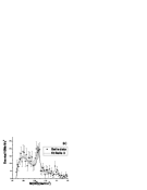
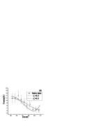
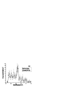
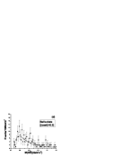
Figure 1: (a)The $M(D\bar{D})$ distribution in $\gamma\gamma\rightarrow D\bar{D}$ of Belle data compared with the result of fit Belle 3. (b) The angular distributions of Belle data compared with fit Belle 2 and fit Belle 3. (c) and (d) are the typical reproduced mass distributions for $|\cos\theta|<0.5$ and $|\cos\theta|>0.5$, respectively, for three fits.

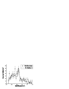
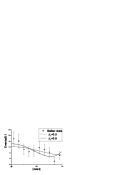
Figure 2: (a)The $M(D\bar{D})$ distribution in $\gamma\gamma\rightarrow D\bar{D}$ of BABAR data compared with the result of fit BABAR 3. (b)The angular distribution of BABAR data compared with the results of fit BABAR 2 and fit BABAR 3.

Without the helicity-2 dominance assumption, we can reexamine the quantum numbers of the $X(3915)$ by incorporating the data for $X\rightarrow J/\psi(\rightarrow l^{+}l^{-})\omega(\rightarrow\pi^{+}\pi^{-}\pi^{0})$ from BABAR. Because of the degeneracy of the $X(3915)$ and the $X(3930)$, we assume that the $X(3915)$ and the $X(3930)$ are the same tensor state and check whether it is consistent with the angular distribution data used by BABAR in determining the quantum numbers of the $X(3915)$.

Let us recall some basic definitions and results from Ref. Rosner (2004). $\theta^{*}_{l}$ is defined as the angle between the momentum of the positively charged lepton from $J/\psi$ decay ($l^{+}$) and the $\gamma\gamma$ axis in the $J/\psi\omega$ rest frame. $\theta^{*}_{n}$ is defined as the angle between the normal to the decay plane of the $\omega$ (defined as $\vec{n}$) and the $\gamma\gamma$ axis in the $J/\psi\omega$ rest frame. $\theta_{ln}$ is the angle between the lepton $l^{+}$ from $J/\psi$ decay and the normal of the $\omega$ decay plane, $\vec{n}$ Lees et al. (2012). The $\theta^{*}_{l}$ and $\theta^{*}_{n}$ angular distributions in $X\rightarrow J/\psi(\rightarrow l^{+}l^{-})\omega(\rightarrow\pi^{+}\pi^{-}\pi^{0})$ for a $2^{++}$ $X$ state produced in a $\gamma\gamma$ collision read

$$\frac{d\Gamma}{d\mathrm{cos}\theta^{*}_{l}} = \frac{1}{8}[6|A_{\pm 2}|^{2}(1+\mathrm{cos}^{2}\theta^{*}_{l})+|A_{0}|^{2}(5-3\mathrm{cos}^{2}\theta^{*}_{l})],$$

$$\frac{d\Gamma}{d\mathrm{cos}\theta^{*}_{n}} = \frac{1}{4}[6|A_{\pm 2}|^{2}(1-\mathrm{cos}^{2}\theta^{*}_{n})+|A_{0}|^{2}(1+3\mathrm{cos}^{2}\theta^{*}_{n})],$$

with the helicity amplitudes $A_{0}$ and $A_{\pm 2}$ suitably normalized, while the $\theta_{ln}$ angular distribution for the decay of a $2^{++}$ $X$ state produced in a $\gamma\gamma$ collision is $\frac{1}{\Gamma}\frac{d\Gamma}{d\mathrm{cos}\theta_{ln}}=\frac{3}{40}[7-\cos^{2}\theta_{ln}]$. The angular distributions of lepton or pion for a $0^{++}$ state do not show any dependence on the angles of $\theta^{*}_{l}$ or $\theta^{*}_{n}$, and the angular dependence for a $0^{++}$ state on $\theta_{ln}$ is $\frac{1}{\Gamma}\frac{d\Gamma}{d\mathrm{cos}\theta_{ln}}=\frac{3}{4}\mathrm{sin}^{2}\theta_{ln}.$

The ratios ${\cal R}$ of the $2^{++}$ intermediate state in $\gamma\gamma\rightarrow J/\psi\omega,D\bar{D}$ are the same according to Eq.(Could the $X(3915)$ and the $X(3930)$ Be the Same Tensor State?) and the pole dominance assumption. We then perform another fit combining the previous $\gamma\gamma\to D\bar{D}$ data and the above three angular-distribution data from $\gamma\gamma\to J/\psi\omega$, setting all the parameters free. Since Belle has no angular-distribution data for $\gamma\gamma\to J/\psi\omega$ channel, we use only BABAR’s data for both channels for consistency. In the combined fit, the $\chi^{2}$ contributed by $\gamma\gamma\to D\bar{D}$ data is $74.7$ which is almost the same as the one for fit BABAR 1. The $\chi^{2}$ for the $\cos\theta_{l}^{*}$ distribution in Fig. 3(a) is improved from 11.2 for $0^{++}$ assignment to 10.1 for $2^{++}$ assignment and the one for $\cos\theta_{n}^{*}$ distribution in Fig. 3(b) is improved from 6.9 to 4.5. In BABAR’s argument, it is just because of the much better $\chi^{2}$ of the dashed line than the dotted line in the second graph that they strongly suggest the $0^{++}$ assignment to $X(3915)$. So, their reasoning is not convincing any more. The angular distribution of the $\cos\theta_{ln}$ does not depend on the helicity since it averages different moving directions of $X(3915)$. The curves in Fig. 3(c) are not fits but predictions. However, the analysis based on these data for $\cos\theta_{ln}$ distribution is not quite reliable. In principle, the distribution must be symmetric with respect to $\cos\theta_{ln}=0$, but in the experimental data in the region $0.6<\cos\theta_{ln}<0.8$ there is no events, while in the mirror region, $-0.8<\cos\theta_{ln}<-0.6$, there are around nine events detected. This clearly demonstrates that the statistics is still too low to produce a good $\cos\theta_{ln}$ distribution. Furthermore, the $\chi^{2}$ also strongly depends on the missing events in Fig. 3(c). In BABAR’s analysis, by setting the data in the region of $0.6<\cos\theta_{ln}<0.8$ to be zero, they obtained that the $\chi^{2}$ for $\cos\theta_{ln}$ in Fig. 3(c) is 18.0 for the $2^{++}$ assignment, worse than 12.5 for the $0^{++}$ assignment. However, as a reasonable assumption, if the data in this region are the same as that of $-0.8<\cos\theta_{ln}<-0.6$ due to the symmetry, the $\chi^{2}$ of $\cos\theta_{ln}$ distribution will be significantly reduced to 10.7 for $2^{++}$ vs 9.2 for $0^{++}$. Because of the apparent poor quality of the $\cos\theta_{ln}$ distribution data, they cannot be used to distinguish which assignment is better. Thus, the total $\chi^{2}/{\rm d.o.f}$ in our analysis improves from $1.50$ for the fit BABAR 1 to about $1.27$, which demonstrates that the experimental data favor the $2^{++}$ assignment of $X(3915)$.

Figure 3: The angular distributions for (a) $\mathrm{cos}\theta^{*}_{l}$, (b) $\mathrm{cos}\theta^{*}_{n}$, and (c) $\mathrm{cos}\theta_{ln}$ of $X(3915)$. Dashed line: intermediate $0^{++}$ resonance; solid line: $2^{++}$ resonance in the combined fit; dotted line : $2^{++}$ resonance with helicity-2 dominance used by BABAR in Ref. Lees et al. (2012).

With the tensor assignment, the $X(3915)$ could be the same state as the $X(3930)$ due to the degeneracies of their masses and widths. Since the global fit automatically produces $\beta_{1}:\beta_{2}\simeq 0.48:0.31$ for the tensor assignment, our result is sufficient to illustrate that, the experimental data prefer a sizable helicity-0 contribution which may even be larger than the helicity-2 contribution. As stated before, the helicity-2 dominance is a consequence of assuming that $X(3915)/X(3930)$ is a quarkonium state Krammer and Krasemann (1978); Li et al. (1991). The large helicity-0 contribution in our scenario means that $X(3915)/X(3930)$ might not be a pure $q\bar{q}$ quarkonium state, but with a significant non-$q\bar{q}$ component. Actually, most charmoniumlike states above the open-charm threshold can hardly be understood as conventional quarkonium states, but can be described well in the spirit of coupled-channel effects Eichten et al. (1978, 1980); Heikkila et al. (1984); van Beveren et al. (1983); Pennington and Wilson (2007); Zhou and Xiao (2014); Danilkin and Simonov (2010) or as molecular states Liang et al. (2010), in which the states contain a significant portion of non-$q\bar{q}$ components.

In conclusion, in this Letter, we present that the $\gamma\gamma\rightarrow D\bar{D},J/\psi\omega$ data favor a possibility that the $X(3915)$, listed in the PDG table as the $\chi_{c0}(2P)$ state, is just the $2^{++}$ state $X(3930)$. The data also prefer that this tensor state has a sizable helicity-0 contribution in the $\gamma\gamma\rightarrow D\bar{D},J/\psi\omega$ amplitudes, comparable to or maybe larger than the helicity-2 contribution. This is a hint of a sizable non-$q\bar{q}$ component in the state. Our results of identifying the $X(3915)$ with the $X(3930)$ and abandoning the helicity-2 dominance may inspire further theoretical and experimental explorations on the properties of the charmoniumlike states.