Relativistic extended coupled cluster method for magnetic hyperfine structure constant

Abstract

The article deals with the general implementation of 4-component spinor relativistic extended coupled cluster (ECC) method to calculate first order property of atoms and molecules in their open-shell ground state configuration. The implemented relativistic ECC is employed to calculate hyperfine structure (HFS) constant of alkali metals (Li, Na, K, Rb and Cs), singly charged alkaline earth metal atoms (Be⁺, Mg⁺, Ca⁺ and Sr⁺) and molecules (BeH, MgF and CaH). We have compared our ECC results with the calculations based on restricted active space configuration interaction (RAS-CI) method. Our results are in better agreement with the available experimental values than those of the RAS-CI values.

I Introduction

The interaction of nuclear moment with the internally generated electromagnetic field by electrons causes small shift and splitting in the energy levels of atom, molecule or ion. This interaction is known as hyperfine structure (HFS) lindgren_book , which plays a key role in atomic clock and laser experiments. A variety of applications including telecommunications, global positioning system, very-long-baseline interferometry telescopes vlbi and test of fundamental concepts of physics fund_phys demand very precise measurement of time, which can be given by an atomic clock, where the unit of time is defined in terms of frequency at which an atom absorbs or emits photon during a particular transition. The laser cooling and atom trapping experiments require the knowledge of HFS as it influences the optical selection rule and the transfer of momentum from photon to the atom. In particular, as the line width of transition of laser is much smaller than the energy difference between two hyperfine labels, the frequency of repumping laser depends on the separation of hyperfine labels Phillips_1998 .

The standard model (SM) of particle physics predicts either a zero or a very small (less than 10^-38 e.cm) electric dipole moment (EDM) of an electron. Therefore, a measurable non-zero EDM of an electron can explore the physics beyond SM. The violation of time reversal (T) or equivalently charge conjugation (C) and spatial parity (P) symmetry of an atomic/molecular system is responsible for the non zero EDM of an electron. Unfortunately, the accuracy of the theoretically estimated P,T -odd interaction constants cannot be mapped with the experiment as there are no corresponding experimental observables. However, the accuracy of theoretically obtained P,T -odd interaction constants can be estimated by comparing theoretically obtained HFS constants with the experimental values as the calculation of both requires an accurate wave function in the nuclear region and the operator forms are more or less similar.

Hyperfine structure as its name suggest, causes very small shift and splitting in the energy levels and thus, the treatment of it requires simultaneous inclusion of both relativistic effects and electron correlation as they are non-additive in nature. The best way to include relativistic effect in a single determinant theory is to solve the Dirac-Hartree-Fock (DHF) Hamiltonian, whereas single reference coupled cluster (SRCC) method is known to be the most efficient to include the dynamic part of the electron correlation bartlett_2007 ; pal_1989 . The SRCC method can be solved either by method of variation or by non-variation. The non-variational solution of SRCC method is the most familiar, known as normal CC (NCC). The NCC, being non-variational, does not have the upper bound property of energy. The generalized Hellmann-Feynman (GHF) theorem and (2n+1) rule, which states that (2n+1)^th order energy derivative can be obtained with the knowledge upto n^th order amplitude derivatives, are not satisfied monkhorst_1977 ; bartlett_1984 . The implication of these theorems save enormous computational effort for the calculation of higher order properties, which clearly a lack in the NCC. However, the energy derivatives within the NCC can be obtained by Z-vector approach zvector_cc or Lagrange multiplier method of Helgaker et al jorgensen_helgaker . However, the GHF theorem and the (2n+1) rule are automatically satisfied in the variational CC (VCC). Among the various VCC methods, expectation value CC (XCC), unitary CC (UCC) and extended CC (ECC) are the most fimiliar in literature. The XCC and UCC use Euler type of functional where the left vector is complex conjugate of the right vector. The detailed discussion on various variational coupled cluster methods can be found in reference rod_xcc1995 . The ECC functional proposed by Arponen and coworkers arponen ; arponen_bishop can bypass all the problems associated with the Euler type of functional by assuming an energy functional which deals with the dual space of both right and left vector in a double linked form. This double linking ensures that the energy and its all order derivatives are size extensive. As the left and right vectors of the ECC functional are not complex conjugates, it contains relatively large variational space as compared to corresponding Euler type functional. The linearized version of ECC, in which the left vector is linear, leads to the equations of NCC pal_lecc . Thus, it can be inferred that ECC wavefunction, which spans more correlated determinantal space than the NCC, eventually improves the correlation energy as well as energy derivatives.

The manuscript is organized as follows. A brief overview of the ECC method including concise details of magnetic HFS constant are described in Sec. II. Computational details are given in Sec. III. We presented our calculated results and discuss about those in Sec. IV before making our concluding remark. We are consistent with atomic unit unless stated.

II Theory

II.1 ECC functional

The ECC functional can be derived by parameterizing both bra and ket states. The parametrization is done by a double similarity transformation that leads to an alternative approach of many body problem where the functional is biorthogonal in nature. It is pertinent to note that the double similarity transformed Hamiltonian is no longer Hermitian as the similarity transformations are not unitary. The ECC functional of an arbitrary operator (A) is given by

$$\langle A\rangle=\frac{\langle\Phi_{0}|e^{\Sigma^{\prime}}Ae^{\Sigma}|\Phi_{0}\rangle}{\langle\Phi_{0}|e^{\Sigma^{\prime}}e^{\Sigma}|\Phi_{0}\rangle},$$ (1)

where $|\Phi_{0}\rangle$ is the DHF reference determinant and $\Sigma^{\prime}$, $\Sigma$ are hole-particle (h-p) destruction and creation operator respectively. Arponen proved that $\langle\Phi_{0}|e^{\Sigma^{\prime}}e^{\Sigma}/\langle\Phi_{0}|e^{\Sigma^{\prime}}e^{\Sigma}|\Phi_{0}\rangle$ can be written as $\langle\Phi_{0}|e^{\Sigma^{\prime{\prime}}}$, where $\Sigma^{\prime{\prime}}$ is h-p destruction operator. Therefore, the ECC functional for the operator becomes

$$\langle A\rangle=\langle\Phi_{0}|e^{\Sigma^{\prime{\prime}}}e^{-\Sigma}Ae^{\Sigma}|\Phi_{0}\rangle.$$ (2)

The diagrammatic structure of $e^{-\Sigma}Ae^{\Sigma}$, which can also be written as $(Ae^{\Sigma})_{c}$ (where c stands for connected), leads to a terminating series. However, the diagrams in which $\Sigma^{\prime{\prime}}$ is solely connected to a single $\Sigma$ leads to disconnected term in the amplitude equation. To avoid this problem, Arponen has defined two sets of amplitudes, $s$ and $t$, with which the functional can be written as

$$\langle A\rangle=\langle\Phi_{0}|e^{S}(Ae^{T})_{L}|\Phi_{0}\rangle_{DL},$$ (3)

where $L$ means that the $T$ operators right side of $A$ are linked to $A$ vertex and $DL$ denotes that a $S$ operator must be connected to either $A$ or at least two $T$ operators. The form of the $S$ and $T$ operators are given by

$$X=\sum\limits_{\stackrel{{\scriptstyle q_{1}<q_{2}\dots}}{{p_{1}<p_{2}\dots}}}t_{p_{1}p_{2}\dots}^{q_{1}q_{2}\dots}{a_{q_{1}}^{\dagger}a_{q_{2}}^{\dagger}\dots a_{p_{2}}a_{p_{1}}},$$ (4)

where X is T when $p$($q$) are hole(particle) index and X is S when $p$($q$) are particle(hole) index.

The analytic energy derivatives can be calculated by using the ECC functional given in equation 3 where the operator is replaced by a perturbed Hamiltonian. The field dependent perturbed Hamiltonian is given by

$$H(\lambda)=H+\lambda O=f+v+\lambda O,$$ (5)

where $H$ is the field independent Hamiltonian, $O$ is an external field and $\lambda$ indicates the strength of the field. $f$ and $v$ are one electron and two electron part of the field independent Hamiltonian respectively. Pal and co-workers pal_ecc_prop have shown that the ECC analytic derivatives can be obtained by expanding the ECC functional as a power series of $\lambda$ and making the functional stationary with respect to cluster amplitudes in progressive orders of $\lambda$. The zeroth order $k$-body cluster amplitudes, which are sufficient to get the first order derivative of energy (which is nothing but the expectation value in the light of GHF theorem), can be obtained by using the following conditions

$$\frac{\delta E^{(0)}}{\delta t_{k}^{(0)}}=0, \,\frac{\delta E^{(0)}}{\delta s_{k}^{(0)}}=0.$$ (6)

Although ECC functional is a terminating series, the natural truncation in the single and double model leads to computationally very costly terms. To avoid the costly terms, we have used the truncation scheme as proposed by Vaval et al, vaval_2013 where the right exponential of the functional is full within the coupled cluster single and double (CCSD) approximation and all the higher order double linked terms within the CCSD approximation are taken in left exponent. The detailed algebraic expression and diagrammatic of the amplitude equations and first order energy derivative are given in Appendix A and Appendix B, including the nuclear magnetic moment $(\mu)$ and spin quantum number (I) of the atoms (in table 4 of Appendix C) and the experimental bond length of molecules used (in table 5 of Appendix C) in our calculation.

Table 1: Magnetic hyperfine structure constant (A) of ground state (${}^{2}S_{1/2}$) of atoms in MHz

Atom	This work		Others	Experiment	$\delta\%$
	RAS-CI	ECC
6Li	148.5	149.3	152.1 yerokhin_2008	152.1 beckmann_1974	1.9
7Li	392.1	394.3	401.7 yerokhin_2008	401.7 beckmann_1974	1.9
23Na	812.1	861.8	888.3 safranova_1999	885.8 beckmann_1974	2.8
39K	188.8	223.5	228.6 safranova_1999	230.8 beckmann_1974	3.3
40K	-234.7	-277.9		-285.7 eisinger_1952	2.8
41K	103.6	122.7		127.0 beckmann_1974	3.5
85Rb	782.3	972.5	1011.1 safranova_1999	1011.9 vanier_1974	4.0
87Rb	2651.0	3295.7		3417.3 essen_1961	3.7
133Cs		2179.1	2278.5 safranova_1999	2298.1 arimondo_1977	5.5
9Be+	-613.7	-614.6	-625.4 yerokhin_2008	-625.0 wineland_1983	1.7
25Mg+	-568.7	-581.6	-593.0 sur_2005	-596.2 itano_1981	2.5
43Ca+	-733.3	-794.9	-805.3 yu_2004	-806.4 arbes_1994	1.4
87Sr+	-872.1	-969.9	-1003.2 yu_2004	-1000.5(1.0)buchinger_1990	3.1

Table 2: Parallel ($A_{\|}$) and perpendicular ($A_{\perp}$) magnetic hyperfine structure constant of molecules in MHz

		A∥					A⟂
Molecule	Atom	This work			Experiment	$\delta\%$	This work			Experiment	$\delta\%$
		SCF	RAS-CI	ECC	weltner_book		SCF	RAS-CI	ECC	weltner_book
BeH	1H	84.2	177.2	204.1	201(1) knight_1972	1.5	65.8	158.7	185.6	190.8(3) knight_1972	2.8
	9Be	-182.7	-203.3	-200.6	-208(1) knight_1972	3.7	-169.4	-188.9	-186.0	-194.8(3) knight_1972	4.7
MgF	19F	168.0	255.4	320.9	331(3) knight_1971a	3.1	99.8	139.4	153.3	143(3) knight_1971a	6.7
	25Mg	-249.2	-272.4	-282.6			-239.4	-260.3	-270.4
CaH	1H	41.1	74.6	146.4	138(1) knight_1971b	5.7	37.5	70.9	141.9	134(1) knight_1971b	5.6
	43Ca	-259.5	-307.9	-321.6			-242.7	-284.6	-295.7

II.2 Magnetic hyperfine interaction constant

The interaction of nuclear magnetic moment with the angular momentum of electrons is responsible for the magnetic HFS. Thus, it can be viewed as a one body interaction from the point of view of the electronic structure theory lindgren_book . The magnetic vector potential $(\vec{A})$ at a distance $\vec{r}$ due to a nucleus $K$ of an atom is

$$\vec{A}=\frac{\vec{\mu}_{k}\times\vec{r}}{r^{3}},$$ (7)

where $\vec{\mu}_{k}$ is the magnetic moment of nucleus $K$. The perturbed HFS Hamiltonian of an atom due to $\vec{A}$ in the Dirac theory is given by $H_{hyp}=\sum_{i}^{n}\alpha_{i}\cdot\vec{A_{i}}$, where $n$ is the total no of electrons and $\alpha_{i}$ denotes the Dirac $\alpha$ matrices for the i^th electron. Now the magnetic hyperfine constant $(A_{J})$ of the $J^{th}$ electronic state of an atom is given by

$$A_{J}=\frac{1}{IJ}\langle\Psi_{J}|H_{hyp}|\Psi_{J}\rangle=\frac{\vec{\mu_{k}}}{IJ}\cdot\langle\Psi_{J}|\sum_{i}^{n}\left(\frac{\vec{\alpha}_{i}\times\vec{r}_{i}}{r_{i}^{3}}\right)|\Psi_{J}\rangle,$$ (8)

where $|\Psi_{J}\rangle$ is the wavefunction of the $J^{th}$ electronic state and $I$ is the nuclear spin quantum number. For a diatomic molecule, the parallel ($A_{\|}$) and perpendicular ($A_{\perp}$) magnetic hyperfine constant can be written as

$$A_{\|(\perp)}=\frac{\vec{\mu_{k}}}{I\Omega}\cdot\langle\Psi_{\Omega}|\sum_{i}^{n}\left(\frac{\vec{\alpha}_{i}\times\vec{r}_{i}}{r_{i}^{3}}\right)_{z(x/y)}|\Psi_{\Omega(-\Omega)}\rangle,$$ (9)

where $\Omega$ represents the z component of the total angular momentum of the diatomic molecule and it takes the value of +1/2 in all the considered cases in this manuscript. It is clear from the above equation that the $A_{\|}$ is proportional to the diagonal matrix elements of $\left(\frac{\vec{\alpha}\times\vec{r}}{r^{3}}\right)_{z}$ but $A_{\perp}$ is proportional to the nondiagonal matrix elements of $\left(\frac{\vec{\alpha}\times\vec{r}}{r^{3}}\right)_{x/y}$ between two different states (+$\Omega$ and -$\Omega$). However, $\Omega$ = +1/2 and -1/2 states are degenerate and their corresponding determinants differ by only one spin up or spin down electron. Thus, the cluster amplitudes are of same magnitude for both $\Omega$ = +1/2 and -1/2 states. So, for each system, cluster amplitudes are evaluated once and they are used to calculate both $A_{\|}$ and $A_{\perp}$ with their corresponding property integrals. However, the rearrangement of the one electron property matrix of $A_{\perp}$ is necessary in the contraction between individual matrix element and proper cluster amplitude.

III Computational details

The DIRAC10 dirac10 package is used to solve the DC Hamiltonian and to obtain one-electron hyperfine integrals. Finite size of nucleus with Gaussian charge distribution is considered as the nuclear model. The nuclear parameters for the Gaussian charge distribution are taken as default values in DIRAC10. Aug-cc-pCVQZ basis aug_ccpcvqz_LiNe ; aug_ccpcvqz_NaMg is used for Li, Be, Na, Mg, F atoms and aug-cc-pCV5Z aug_ccpcvqz_LiNe is used for H atom. We have used dyall.cv4z dyall_4s7s basis for K, Ca and Cs atoms and dyall.cv3z dyall_4s7s basis for Rb and Sr atoms. All the occupied orbitals are taken in our calculations. The virtual orbitals whose energy exceed a certain threshold (see in table 6 of Appendix C) are not taken into account in our calculations as the contribution of high energy virtual orbitals is negligible in the correlation calculation. Restricted active space configuration interaction (RAS-CI) calculations are done using a locally modified version of DIRAC10 package and the detailed description of RAS configuration is compiled in table 6 of Appendix C.

IV Results and discussion

The numerical results of our calculations of HFS constant using 4-component spinor ECC method, capable of treating ground state open-shell configuartion are presented. We also present results using RAS-CI method. The RAS-CI calculations are done using DIRAC10 package.

In Table 1, we present the HFS constant values of alkali metal atoms starting from Li to Cs and singly charged alkaline earth metal atoms (Be⁺ to Sr⁺). Our results are compared with the available experimental values and the values calculated using RAS-CI method. The deviation of our ECC values from the experimental values are presented as $\delta\%$. Our ECC results are in good agreement with the experimental results ($\delta\%$ $<$ 6$\%$). It is observed that the deviations increase as we go down both in the alkali metal and in alkaline earth metal group of the periodic table except for the Ca⁺ ion in the series. The deviations of RAS-CI and ECC values with the experimental values are presented in Fig 1.

Table 3: HFS constant of ${}^{1}H$ of CaH molecule in RAS-CI method.

Basis			A∥ (MHz)				A⟂ (MHz)
Ca	H	Spinor	SCF	Correlation	Total	Experiment	SCF	Correlation	Total	Experiment
dyall.v3z	cc-pVTZ	192	38.9	35.3	74.2	×	35.3	35.4	70.7	×
dyall.cv3z	aug-cc-pCV5Z	274	41.2	33.4	74.6	138(1) weltner_book ; knight_1971a	37.5	33.4	70.9	134(1) weltner_book ; knight_1971a
dyall.cv3z	aug-cc-pCV5Z	318	41.2	34.0	75.2	×	37.5	34.1	71.6	×

It is clear that the deviations of RAC-CI are always greater than ECC and it is expected as the coupled cluster is a better correlated theory than the truncated CI theory. It is interesting to note that the deviations in RAS-CI increase much faster rate compared to ECC as we go down the groups. This reflect the fact that truncated CI is not size extensive and thus it does not scale properly with the increasing number of electrons. It should be noted that the ratio of theoretically estimated HFS constant of different isotopes must be the ratio of their nuclear g factor for point nuclear model. Different isotopes are treated by changing the nuclear magnetic moment $(\mu)$ of the atom but nuclear parameters for each isotopes are same which is by default of the most stable isotopes in DIRAC10. This causes difference in $\delta\%$ of different isotopes.

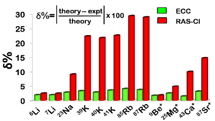
Figure 1: Comparison of relative deviations between ECC and RAS-CI values of our calculations.

In Table 2, we present the parallel and perpendicular HFS constant of ground state of BeH, MgF and CaH molecules obtained from RAS-CI and ECC theory. We have compared our ECC results with the available experimental values and the deviations are reported as $\delta\%$. Our calculated results within the ECC framework show good agreement with the experimental values. The highest deviation for parallel HFS constant is in the case of ¹H of CaH where the ECC value differs only $\sim$ 8.5 MHz. This is also better than the RAS-CI values where the deviation is too off ($\sim$ 63.5 MHz) from the experimental values. However, for ⁹Be in BeH and ¹⁹F in MgF, RAS-CI yields marginally better results ($\sim$ 10 MHz) as compared to ECC.

Like the RAS-CI parallel HFS constant values of ¹H of CaH, the perpendicular HFS constant is very off from the experimental values. To investigate this, we have calculated the HFS of CaH with more number of virtual orbitals in the same as well as with a different basis. The results are presented in table 3. It is clear from Table 3 that for this system RAS-CI gives very bad estimation of HFS constant. A possible explanation is as follows, according to Kutzelnigg’s error analysis kutzelnigg_1991 the comparative error in CI energy can be written as [O($\delta$ + O(S²))]² where $e^{S}$ is the wave operator of NCC method and $\delta$ is the error of the wave operator. Although the comparative error analysis of CI by Kutzelnigg is with respect to NCC but we expect a similar expression will be hold for ECC also. From Table 3, it is clear that the DHF (SCF) contribution to the energy derivative is significantly less whereas the correlation contribution for ECC to the energy derivative is very large as compared to SCF contribution which is evident from table 2. Therefore, the DHF ground state is very poor reference for this system and for ECC, the wave operator must be large enough. Thus, it associates considerably large error in the CI energy as the error in CI energy is proportional to the quartic of wave operator of CC wave function.

It is interesting to see that both the parallel and perpendicular HFS of ¹H decrease as we go from BeH to CaH. This indicates that the spin density near ¹H nucleus of CaH is less than that of BeH. This explains the ionicity of the bond in CaH is greater than the bond in BeH.

We have done series of calculations to estimate uncertainty in our calculations by comparing our ECC results with FCI results taking example of ⁷Li, ⁹Be and BeH. Details of the these calculations are included in Appendix D. We believe that the uncertainty in our calculations with respect to full CI results for the atomic systems are well within 5% and 10% for the molecular systems considering all possible sources of error in our calculations.

V Conclusion

We have successfully implemented the relativistic ECC method using 4-component Dirac spinors to calculate first order energy derivatives of atoms and molecules in their open-shell ground state configuration. We applied this method to calculate the magnetic HFS constant of Li, Na, K, Rb, Cs, Be⁺, Mg⁺, Ca⁺ and Sr⁺ along with parallel and perpendicular magnetic HFS constant of BaH, MgF and CaH molecules. We also present RAS-CI results to show the effect of correlation in the calculation of HFS constant. Our ECC results are in good agreement with the experiment. We have found some anomalies in RAS-CI results of CaH and given a possible explanation.

Appendix A Algebraic expression of ECC energy and cluster amplitude equation

The zeroth order ECC energy functional within the approximation stated in the manuscript is

$$\begin{split}E^{(0)}=&\langle\Phi_{0}|\Big{[}vt_{2}^{(0)}+s_{2}^{(0)}v+s_{1}^{(0)}ft_{1}^{(0)}+s_{2}^{(0)}ft_{2}^{(0)}+s_{1}^{(0)}vt_{1}^{(0)}+s_{2}^{(0)}vt_{2}^{(0)}+s_{2}^{(0)}vt_{1}^{(0)}+s_{1}^{(0)}vt_{2}^{(0)}+\frac{1}{2!}vt_{1}^{(0)}t_{1}^{(0)}\\ &+\frac{1}{2!}s_{1}^{(0)}s_{1}^{(0)}v+\frac{1}{2!}s_{1}^{(0)}vt_{1}^{(0)}t_{1}^{(0)}+\frac{1}{2!}s_{1}^{(0)}s_{1}^{(0)}vt_{1}^{(0)}+s_{1}^{(0)}vt_{1}^{(0)}t_{2}^{(0)}+s_{2}^{(0)}vt_{1}^{(0)}t_{2}^{(0)}+\frac{1}{2!}s_{2}^{(0)}vt_{2}^{(0)}t_{2}^{(0)}\\ &+s_{1}^{(0)}s_{2}^{(0)}vt_{2}^{(0)}+\frac{1}{3!}s_{2}^{(0)}v(t_{1}^{(0)})^{3}+\frac{1}{2!}s_{2}^{(0)}vt_{2}^{(0)}(t_{1}^{(0)})^{2}+\frac{1}{4!}s_{2}^{(0)}v(t_{1}^{(0)})^{4}+\frac{1}{3!}(s_{1}^{(0)})^{3}vt_{2}^{(0)}+ft_{1}^{(0)}\\ &+s_{1}^{(0)}f+\frac{1}{2!}s_{1}^{(0)}f(t_{1}^{(0)})^{2}+s_{2}^{(0)}ft_{1}^{(0)}t_{2}^{(0)}+\frac{1}{3!}s_{1}^{(0)}v(t_{1}^{(0)})^{3}\Big{]}|\Phi_{0}\rangle.\end{split}$$ (10)

Equation for $s_{1}^{(0)}[\delta E^{(0)}/\delta t_{1}^{(0)}=0]$ is given by

$$\begin{split}\langle\Phi_{0}|\Big{[}&vt_{1}^{(0)}+s_{1}^{(0)}(f+v)+s_{2}^{(0)}v+s_{1}^{(0)}vt_{1}^{(0)}+s_{1}^{(0)}vt_{2}^{(0)}+s_{2}^{(0)}vt_{1}^{(0)}+s_{2}^{(0)}vt_{2}^{(0)}+\frac{1}{2!}s_{1}^{(0)}s_{1}^{(0)}v+s_{2}^{(0)}vt_{2}^{(0)}t_{1}^{(0)}\\ &+\frac{1}{2!}s_{2}^{(0)}vt_{1}^{(0)}t_{1}^{(0)}+\frac{1}{3!}s_{2}^{(0)}v(t_{1}^{(0)})^{3}+f+s_{1}^{(0)}ft_{1}^{(0)}+s_{2}^{(0)}ft_{2}^{(0)}+\frac{1}{2!}s_{1}^{(0)}vt_{1}^{(0)}t_{1}^{(0)}\Big{]}|\Phi_{i}^{a}\rangle=0.\end{split}$$ (11)

Equation for $s_{2}^{(0)}[\delta E^{(0)}/\delta t_{2}^{(0)}=0]$ is given by

$$\begin{split}\langle\Phi_{0}|\Big{[}&v+s_{1}^{(0)}v+s_{2}^{(0)}(f+v)+\frac{1}{2!}s_{1}^{(0)}s_{1}^{(0)}v+s_{1}^{(0)}s_{2}^{(0)}v+s_{1}^{(0)}vt_{1}^{(0)}+s_{2}^{(0)}vt_{1}^{(0)}+s_{2}^{(0)}vt_{2}^{(0)}+\frac{1}{2!}s_{2}^{(0)}vt_{1}^{(0)}t_{1}^{(0)}\\ &+\frac{1}{3!}(s_{1}^{(0)})^{3}v+s_{2}^{(0)}ft_{1}^{(0)}\Big{]}|\Phi_{ij}^{ab}\rangle=0.\end{split}$$ (12)

Equation for $t_{1}^{(0)}[\delta E^{(0)}/\delta s_{1}^{(0)}=0]$ is given by

$$\begin{split}\langle\Phi_{i}^{a}|\Big{[}&(f+v)t_{1}^{(0)}+vt_{2}^{(0)}+\frac{1}{2!}vt_{1}^{(0)}t_{1}^{(0)}+vt_{1}^{(0)}t_{2}^{(0)}+s_{1}^{(0)}v+s_{1}^{(0)}vt_{1}^{(0)}+s_{1}^{(0)}vt_{2}^{(0)}+s_{2}^{(0)}vt_{2}^{(0)}+s_{1}^{(0)}s_{1}^{(0)}vt_{2}^{(0)}\\ &+f+\frac{1}{2!}ft_{1}^{(0)}t_{1}^{(0)}+\frac{1}{3!}v(t_{1}^{(0)})^{3}\Big{]}|\Phi_{0}\rangle=0.\end{split}$$ (13)

Equation for $t_{2}^{(0)}[\delta E^{(0)}/\delta s_{2}^{(0)}=0]$ is given by

$$\begin{split}\langle\Phi_{ij}^{ab}|\Big{[}&v+vt_{1}^{(0)}+(f+v)t_{2}^{(0)}+\frac{1}{2!}vt_{1}^{(0)}t_{1}^{(0)}+vt_{1}^{(0)}t_{2}^{(0)}+\frac{1}{2!}vt_{2}^{(0)}t_{2}^{(0)}+\frac{1}{2!}vt_{2}^{(0)}t_{1}^{(0)}t_{1}^{(0)}+\frac{1}{3!}v(t_{1}^{(0)})^{3}+\frac{1}{4!}v(t_{1}^{(0)})^{4}\\ &+ft_{1}^{(0)}t_{2}^{(0)}+s_{1}^{(0)}vt_{2}^{(0)}\Big{]}|\Phi_{0}\rangle=0.\end{split}$$ (14)

Equation for $E^{(1)}$ is given by

$$\begin{split}E^{(1)}=&\langle\Phi_{0}|\Big{[}Ot_{1}^{(0)}+s_{1}^{(0)}O+s_{1}^{(0)}Ot_{1}^{(0)}+s_{2}^{(0)}Ot_{2}^{(0)}+\frac{1}{2!}s_{1}^{(0)}Ot_{1}^{(0)}t_{1}^{(0)}+s_{2}^{(0)}Ot_{1}^{(0)}t_{2}^{(0)}\Big{]}|\Phi_{0}\rangle.\end{split}$$ (15)

Appendix B Diagrammatic of amplitude equation and energy derivative of ECC

In Fig. 2, Fig. 3, Fig. 4 and Fig. 5, we present all the necessary diagrams required to construct the equations for s₁, s₂, t₁ and t₂ amplitudes respectively. The diagrams required for first order energy derivative (E⁽¹⁾) are given in Fig. 6.

Figure 2: Diagrams for s₁ amplitude

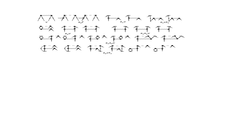
Figure 3: Diagrams for s₂ amplitude

Figure 4: Diagrams for t₁ amplitude

Figure 5: Diagrams for t₂ amplitude

Figure 6: Diagrams for first order energy derivative (E⁽¹⁾)

Appendix C Nuclear parameters of the atoms, bond length of the molecules, RAS-CI configuration and threshold energy of atoms and molecules

The nuclear magnetic moment $(\mu)$ and nuclear spin quantum number of atoms used in our calculations are presented in table 4. The experimental bond length for the molecular system are presented in table 5. RAS-CI configuration and threshold energy for the correlation calculation of the atomic and molecular system are compiled in table 6.

Table 4: Nuclear magnetic moment ($\mu$) and nuclear spin quantum no (I) of atoms mu_I .

Atom

1H

2D

6Li

7Li

9Be

19F

23Na

25Mg

39K

40K

41K

43Ca

85Rb

87Rb

87Sr

I

1/2

1

1

3/2

3/2

1/2

3/2

5/2

3/2

4

3/2

7/2

5/2

3/2

9/2

$\mu/\mu_{N}$

2.7928

0.8574

0.8220

3.2564

-1.1779

2.6288

2.2175

-0.8554

0.3914

-1.2981

0.2149

-1.3172

1.3530

2.7512

-1.0928

Table 5: Bond length of the molecules in Å

Molecule	Bond length bondlen
BeH	1.343
MgF	1.750
CaH	2.003

Table 6: RAS-CI configuration and threshold energy of atoms and molecules

Atom/Molecule	RAS Configurationa		Threshold energyb
×	RAS I	RAS II	(a.u.)
Li	2, 1	3, 4	$\infty$
Na	6, 5	3, 4	$\infty$
K	10, 9	3, 4	500
Rb	19, 18	3, 4	500
Cs	×	×	60
Be+	2, 1	3, 4	$\infty$
Mg+	6, 5	3, 4	$\infty$
Ca+	10, 9	3, 4	500
Sr+	19, 18	3, 4	100
BeH	3, 2	3, 4	$\infty$
MgF	11, 10	3, 4	10
CaH	11, 10	5, 6	15

^a In each RAS configuration spin up and spin down spinors are seperated by comma.
Maximum number of holes in RAS I is 2. Maximum number of electrons in RAS III is 2.
^b $\infty$ value means all the spinors are considered in the correlation calculation.

Appendix D Comparison of full CI and ECC HFS constant values

The comparison of full CI and ECC HFS constant values of ⁷Li and ⁹Be⁺ is presented in table 7 and table 8 respectively. The comparison of parallel and perpendicular component of full CI and ECC HFS constant values of BeH is compiled in table 9.

Table 7: Comparison of full CI and ECC HFS values (in MHz) of ⁷Li

Basis	Full CI	ECC
aug-cc-pCVDZ	384.1	383.9
aug-cc-pCVTZ	402.0	401.5
aug-cc-pCVQZa	386.0	385.5

^a Considering 3 electrons and 189 virtual orbitals

Table 8: Comparison of full CI and ECC HFS values (in MHz) of ⁹Be⁺

Basis	Full CI	ECC
aug-cc-pCVDZ	-586.6	-586.5
aug-cc-pCVTZ	-615.7	-615.6
aug-cc-pCVQZa	-613.0	-612.8

^a Considering 3 electrons and 183 virtual orbitals

Table 9: Comparison of full CI and ECC HFS values (in MHz) of BeH.

Basis	Atom	$A_{\|}$		$A_{\perp}$
×	×	Full CI	ECC	Full CI	ECC
cc-pVDZ	9Be	-158.7	-159.3	-145.9	-146.6
×	1H	189.9	187.6	174.5	172.2
aug-cc-pVDZ	9Be	-165.5	-166.1	-152.6	-153.2
×	1H	188.7	186.2	172.1	169.7

References

- (1) I. Lindgren and J. Morrison, Atomic Many-Body Theory (Springer-Verlag, New York).
- (2) D. Normile and D. Clery, Science 333, 1820 (2011).
- (3) T. Rosenband et al, Science 319, 1808 (2008).
- (4) W. D. Phillips, Reviews of Modern Physics 70, 721 (1998).
- (5) R. J. Bartlett and M. Musiał, Rev. Mod. Phys. 79, 291 (2007).
- (6) D. Mukherjee and S. Pal, Adv. Quantum Chem. 20, 291 (1989).
- (7) J. H. Monkhorst, Int. J. Quantum Chem. 12, 421 (1977).
- (8) H. Sekino and R. J. Bartlett, Int. J. Quantum Chem. 26, 255 (1984).
- (9) E. A. Salter, G. W. Trucks, and R. J. Bartlett, J. Chem. Phys. 90, 1752 (1989).
- (10) H. Koch, J. A. Jensen, P. Jorgensen, T. Helgaker, G. E. Scuseria, and H. F. Schaefer III, J. Chem. Phys. 92, 4952 (1990)
- (11) P. G. Szalay, M. Nooijen, and R. J. Bartlett, J. Chem. Phys. 103, 281 (1995).
- (12) J. Arponen, Ann. Phys. 151, 311 (1983).
- (13) R. Bishop, J. Arponen, and P. Pajanne, Aspects of Many- body Effects in Molecules and Extended Systems , Lecture Notes in Chemistry Vol. 50 (Springer-Verlag, Berlin, 1989)
- (14) S. Pal, Phys. Rev. A 39, 2712 (1989).
- (15) N. Vaval, K. B. Ghose, and S. Pal, J. Chem. Phys. 101, 4914 (1994).
- (16) S. P. Joshi and N. Vaval, Chem. Phys. Letters, 568, 170 (2013).
- (17) DIRAC, a relativistic ab initio electronic structure program, Release DIRAC10 (2010), written by T. Saue, L. Visscher and H. J. Aa. Jensen, with contributions from R. Bast, K. G. Dyall, U. Ekström, E. Eliav, T. Enevoldsen, T. Fleig, A. S. P. Gomes, J. Henriksson, M. Iliaš, Ch. R. Jacob, S. Knecht, H. S. Nataraj, P. Norman, J. Olsen, M. Pernpointner, K. Ruud, B. Schimmelpfennig, J. Sikkema, A. Thorvaldsen, J. Thyssen, S. Villaume, and S. Yamamoto. (see http://dirac.chem.vu.nl).
- (18) T. H. Dunning, Jr, J. Chem. Phys. 90, 1007 (1989).
- (19) D. E. Woon and T. H. Dunning, Jr. (to be published).
- (20) K.G. Dyall, J. Phys. Chem. A, 113, 12638 (2009).
- (21) V. A. Yerokhin, Phys. Rev. A 78, 012513 (2008).
- (22) A. Beckmann, K. D. Böklen, and D. Elke, Z. Phys. 270, 173 (1974).
- (23) M. S. Safronova, W. R. Johnson, and A. Derevianko, Phys. Rev. A 60, 4476 (1999).
- (24) J. T. Eisinger, B. Bederson, and B. T. Feld, Phys. Rev. 86, 73 (1952).
- (25) J. Vanier, J. F. Simard, and J. S. Boulanger, Phys. Rev. A 9, 1031 (1974).
- (26) L. Essen, E. G. Hope, and D. Sutcliffe, Nature 189, 298 (1961).
- (27) E. Arimondo, M. Inguscio, and P. Violino, Rev. Mod. Phys. 49, 31 (1977).
- (28) D. J. Wineland, J. J. Bollinger, and W. M. Itano, Phys. Rev. Lett. 50, 628 (1983).
- (29) C. Sur, B.K. Sahoo, R.K. Chaudhuri, B.P. Das, and D. Mukherjee, Eur. Phys. J. D 32, 25 (2005).
- (30) W. M. Itano and D.J. Wineland, Phys. Rev. A 24, 1364 (1981).
- (31) K. Z. Yu, L. J. Wu, B. C. Gou, and T. Y. Shi, Phys. Rev. A 70, 012506 (2004).
- (32) F. Arbes, M. Benzing, Th. Gudjons, F. Kurth, and G. Werth, Z. Phys. D 31, 27 (1994).
- (33) F. Buchinger et al, Phys. Rev. C 41, 2883 (1990).
- (34) W. Weltner, Magnetic Atoms and Molecules (Dover Publications Inc., New York, 1983).
- (35) L. B. Knight, Jr., J. M. Brom, Jr., and W. Weltner, Jr., J. Chem. Phys. 56, 1152 (1972).
- (36) L. B. Knight, Jr., W. C. Easley, W. Weltner Jr., and M. Wilson, J. Chem. Phys. 54, 322 (1971)
- (37) L. B. Knight, Jr. and William Weltner, Jr., J. Chem. Phys. 54, 3875 (1971).
- (38) W. Kutzelnigg, Theor. Chim. Acta 80, 349 (1991).
- (39) http://www.webelements.com/isotopes.html
- (40) http://ccbdb.nist.gov/