Fast forward feature selection for the nonlinear classification of hyperspectral images

Abstract

A fast forward feature selection algorithm is presented in this paper. It is based on a Gaussian mixture model (GMM) classifier. GMM are used for classifying hyperspectral images. The algorithm selects iteratively spectral features that maximizes an estimation of the classification rate. The estimation is done using the k-fold cross validation. In order to perform fast in terms of computing time, an efficient implementation is proposed. First, the GMM can be updated when the estimation of the classification rate is computed, rather than re-estimate the full model. Secondly, using marginalization of the GMM, sub models can be directly obtained from the full model learned with all the spectral features. Experimental results for two real hyperspectral data sets show that the method performs very well in terms of classification accuracy and processing time. Furthermore, the extracted model contains very few spectral channels.

I Introduction

Since the pioneer paper of J. Jimenez and D. Landgrebe [1], it is well known that hyperspectral images need specific processing techniques because conventional ones made for multispectral/panchromatic images do not adapt well to hyperspectral images. Generally speaking, the increasing number of spectral channels poses theoretical and practical problems [2]. In particular, for the purpose of pixel classification, the spectral dimension needs to be handle carefully because of the “Hughes phenomenon” [3]: with a limited training set, beyond a certain number of spectral features, a reliable estimation of the model parameters is not possible.

Many works have been published since the 2000s to address the problem of classifying hyperspectral images. A non-exhaustive list should include techniques from the machine learning theory (Support Vector Machines, Random Forest, neural networks) [4], statistical models [1] and dimension reduction [5]. SVM, and kernel methods in general, have shown remarkable performances on hyperspectral data in terms of classification accuracy [6]. However, these methods may suffer from a high computational load and the interpretation of the model is usually not trivial.

In parallel to the emergence of kernel methods, the reduction of the spectral dimension has received a lot of attention. According to the absence or presence of training set, the dimension reduction can be unsupervised or supervised. The former try to describe the data with a lower number of features that minimize a reconstruction error measure, while the latter try to extract features that maximize the separability of the classes. One of the most used unsupervised feature extraction method is the principal component analysis (PCA) [1]. But it has been demonstrated that PCA is not optimal for the purpose of classification [7]. Supervised method, such as the Fisher discriminant analysis or the non-weighted feature extraction have shown to perform better for the purpose of classification. Other feature extraction techniques, such as independent component analysis [8], have been applied successfully and demonstrate that even SVM can benefits from feature reduction [9, 10]. However, conventional supervised techniques suffer from similar problems than classification algorithms in high dimensional space.

Rather than supervised and unsupervised techniques, one can also distinguish dimension reduction techniques into feature extraction and feature selection. Feature extraction returns a linear/nonlinear combination of the original features, while feature selection returns a subset of the original features. While feature extraction and feature selection both reduce the dimensionality of the data, the latter is much more interpretable for the end-user. The extracted subset corresponds to the most important features for the classification, i.e., the most important wavelengths. For some applications, these spectral channels can be used to infer mineralogical and chemical properties [11].

Feature selection techniques generally need a criterion, that evaluates how the model built with a given subset of features performs, and an optimization procedure that tries to find the subset of features that maximizes/minimizes the criterion [12]. Several methods have been proposed according to that setting. For instance, an entropy measure and a genetic algorithm have been proposed in [13, Chapter 9], but the band selection was done independently of the classifier, i.e., the criterion was not directly related to the classification accuracy. Jeffries Matusita (JM) distance and steepest-ascent like algorithms were proposed in [14]. The method starts with a conventional sequential forward selection algorithm, then the obtained set of features is updated using local search. The method has been extended to take into account spatial variability between features in [15] where a multiobjective criterion was used to take into account the class separability and the spatial variability. JM distance and exhaustive search as well as some refinement techniques have been proposed also in [12]. However rather than extracting spectral features, the algorithm returns the average over a certain bandwidth of contiguous channels, which can make the interpretation difficult and often leads to select a large part of the electromagnetic spectrum. Similarly, spectral intervals selection was proposed in [16], where the criterion used was the square representation error (square error between the approximate spectra and the original spectra) and the optimization problem was solved using dynamic programming. These two methods reduce the dimensionality of the data, but cannot be used to extract spectral variables. Recently, forward selection and genetic algorithm driven by the classification error minimization has been proposed in [17].

Feature selection has been also proposed for kernel methods. A recursive scheme used to remove features that exhibit few influence on the decision function of a nonlinear SVM was discussed in [18]. Alternatively, a shrinkage method based on $\ell_{1}$-norm and linear SVM has been investigated by Tuia et al. [19]. The authors proposed a method where the features are extracted during the training process. However, to make the method tractable in terms of computational load, a linear model is used for the classification, that can limit the discriminating power of the classifier. In [20], a dependence measure between spectral features and thematic classes is proposed using kernel evaluation. The measure has the advantage to apply to multiclass problem making the interpretation of the extracted features easier.

Feature selection usually provides good results in terms of classification accuracy. However, several drawbacks can be identified from the above mentioned literature:

• It can be very time consuming, in particular when nonlinear classification models are used.

• When linear models are used for the selection of features, performances in terms of classification accuracy are not satisfying and therefore another nonlinear classifier should be used after the feature extraction.

• For multiclass problem, it is sometimes difficult to interpret the extracted features when a collection of binary classifiers is used (e.g., SVM).

In this work, it is proposed to use a forward strategy, based on [21], that uses an efficient implementation scheme and allows to process a large amount of data, both in terms of number of samples and variables. The method, called nonlinear parsimonious feature selection (NPFS), selects iteratively a spectral feature from the original set of features and adds it to a pool of selected features. This pool is used to learn a Gaussian mixture model (GMM) and each feature is selected according to a classification rate. The iteration stops when the increased in terms of classification rate is lower than a user defined threshold or when the maximum number of features is reached. In comparison to other feature extraction algorithms, the main contributions of NPFS is the ability to select spectral features through a nonlinear classification model and its high computational efficiency. Furthermore, NPFS usually extracts a very few number of features (lower than 5 % of the original number of spectral features).

The remaining of the paper is organized as follows. Section II presents the algorithm with the Gaussian mixture model and the efficient implementation. Experimental results on three hyperspectral data sets are presented and discussed in Section III. Conclusions and perspectives conclude the paper in Section IV.

II Non linear parsimonious feature selection

The following notations are used in the remaining of the paper. $\mathcal{S}=\big{\{}\mathbf{x}_{i},y_{i}\big{\}}_{i=1}^{n}$ denotes the set of training pixels, where $\mathbf{x}_{i}\in\mathbb{R}^{d}$ is a $d$-dimensional pixel vector, $y_{i}=1,\ldots,C$ is its corresponding class, $C$ the number of classes, $n$ the total number of training pixels and $n_{c}$ the number of training pixels in class $c$.

II-A Gaussian mixture model

For a Gaussian mixture model, it is supposed that the observed pixel is a realization of a $d$-dimensional random vector such as

$$p(\mathbf{x})=\sum_{c=1}^{C}\pi_{c}p(\mathbf{x}|c),$$ (1)

where $\pi_{c}$ is the proportion of class $c$ ($0\leq\pi_{c}\leq 1$ and $\sum_{c=1}^{C}\pi_{c}=1$) and $p(\mathbf{x}|c)$ is a $d$-dimensional Gaussian distribution, i.e.,

$$p(\mathbf{x}|c)=\frac{1}{(2\pi)^{d/2}|\boldsymbol{\Sigma}_{c}|^{1/2}}\exp\left(-\frac{1}{2}(\mathbf{x}-\boldsymbol{\mu}_{c})^{T}\boldsymbol{\Sigma}_{c}^{-1}(\mathbf{x}-\boldsymbol{\mu}_{c})\right).$$

with $\boldsymbol{\mu}_{c}$ being the mean vector of class $c$, $\boldsymbol{\Sigma}_{c}$ being the covariance matrix of class $c$ and $|\boldsymbol{\Sigma}_{c}|$ its determinant. Following the maximum a posteriori rule, a given pixel is classified to the class $c$ if $p(c|\mathbf{x})\geq p(k|\mathbf{x})$ for all $k=1,\ldots,C$. Using the Bayes formula, the posterior probability can be written as

$$p(c|\mathbf{x})=\frac{\pi_{c}p(\mathbf{x}|c)}{\sum_{k=1}^{C}\pi_{k}p(\mathbf{x}|k)}.$$ (2)

Therefore, the maximum a posteriori rule can be written as

$$\mathbf{x}\text{ belongs to }c\Leftrightarrow c=\arg\max_{k=1,\ldots,C}\pi_{k}p(\mathbf{x}|k).$$ (3)

By taking the log of eq. (3) the final decision rule is obtained (also known as quadratic discriminant function)

$$Q_{c}(\mathbf{x})=-(\mathbf{x}-\boldsymbol{\mu}_{c})^{T}\boldsymbol{\Sigma}_{c}^{-1}(\mathbf{x}-\boldsymbol{\mu}_{c})-\ln(|\boldsymbol{\Sigma}_{c}|)+2\ln(\pi_{c}).$$ (4)

Using standard maximization of the log-likelihood, the estimator of the model parameters are given by

$$\hat{\pi}_{c} = \frac{n_{c}}{n},$$ (5)

$$\hat{\boldsymbol{\mu}}_{c} = \frac{1}{n_{c}}\sum_{i=1}^{n_{c}}\mathbf{x}_{i},$$ (6)

$$\hat{\boldsymbol{\Sigma}}_{c} = \frac{1}{n_{c}}\sum_{i=1}^{n_{c}}(\mathbf{x}_{i}-\hat{\boldsymbol{\mu}}_{c})(\mathbf{x}_{i}-\hat{\boldsymbol{\mu}}_{c})^{T}.$$ (7)

with $n_{c}$ is the number of sample of class $c$.

For GMM, the “Hughes phenomenon” is related to the estimation of the covariance matrix. If the number of training samples is not sufficient for a good estimation the computation of the inverse and of the determinant in eq.(4) will be very numerically unstable, leading to poor classification accuracy. For instance for the covariance matrix, the number of parameters to estimate is equal to $d(d+1)/2$: if $d=100$ then $5050$ parameters have to be estimated then the minimum number of training samples for the considered class should be at least $5050$. Note in that case the estimation will be possible but not accurate. Feature selection tackles this problem by allowing the construction of GMM with a reduced number $p$ of variables, with $p<<d$ and $p(p+1)/2<n_{c}$.

II-B Forward feature selection

The forward feature selection works as follow [22, Chapter 3]. It starts with an empty pool of selected features. At each step, the feature that most improves an estimation of the classification rate is added to the pool. The algorithm stops either if the increase of the estimated classification rate is too low or if the maximum number of features is reached.

The $k$-fold cross-validation ($k$-CV) is used in this work to estimate the classification rate. To compute the $k$-CV, a subset is removed from $\mathcal{S}$ and the GMM is learned with the remaining training samples. A test error is computed with the removed training samples used as validation samples. The process is iterated $k$ times and the estimated classification rate is computed as the mean test error over the $k$ subsets of $\mathcal{S}$.

The efficient implementation of the NPFS relies on a fast estimation of the parameters of the GMM when the $k$-CV is computed. In the following, it will be shown that by using update rules of the parameters and the marginalization properties of the Gaussian distribution, it is possible to perform $k$-CV and forward selection quickly. As a consequence, the GMM model is learned only one time during the whole training step. The algorithm 1 presents a pseudo code of the proposed method.

II-B1 Fast estimation of the model on $\mathcal{S}^{n-\nu}$

In this subsection, it is shown that each parameter can be easily updated when a subset is taken off $\mathcal{S}$.

Proposition 1 (Proportion)

The update rule for the proportion is

$$\hat{\pi}_{c}^{n-\nu}=\frac{n\hat{\pi}_{c}^{n}-\nu_{c}}{n-\nu}$$ (8)

where $\hat{\pi}_{c}^{n-\nu}$ and $\hat{\pi}_{c}^{n}$ are the proportions of class $c$ computed over $n-\nu$ and $n$ respectively, $\nu$ is the number of removed samples from $\mathcal{S}$, $\nu_{c}$ is the number of removed samples from class $c$ such as $\sum_{c=1}^{C}\nu_{c}=\nu$.

Proposition 2 (Mean vector)

The update rule for the mean vector is

$$\hat{\boldsymbol{\mu}}_{c}^{n_{c}-\nu_{c}}=\frac{n_{c}\hat{\boldsymbol{\mu}}_{c}^{n_{c}}-\nu_{c}\hat{\boldsymbol{\mu}}_{c}^{\nu_{c}}}{n_{c}-\nu_{c}}$$ (9)

where $\hat{\boldsymbol{\mu}}_{c}^{n_{c}}$ and $\hat{\boldsymbol{\mu}}_{c}^{n_{c}-\nu_{c}}$ are the mean vectors of class $c$ computed over the $n_{c}$ and $n_{c}-\nu_{c}$ training samples respectively, $\hat{\boldsymbol{\mu}}_{c}^{\nu_{c}}$ is the mean vector of the $\nu_{c}$ removed samples from class $c$.

Proposition 3 (Covariance matrix)

The update rule for the covariance matrix is

$$\hat{\boldsymbol{\Sigma}}^{n_{c}-\nu_{c}}_{c}=\frac{n_{c}}{(n_{c}-\nu_{c})}\hat{\boldsymbol{\Sigma}}^{n_{c}}_{c}-\frac{\nu_{c}}{(n_{c}-\nu_{c})}\hat{\boldsymbol{\Sigma}}^{\nu_{c}}_{c}-\frac{n_{c}\nu_{c}}{(n_{c}-\nu_{c})^{2}}\left(\hat{\boldsymbol{\mu}}_{c}^{n_{c}}-\hat{\boldsymbol{\mu}}_{c}^{\nu_{c}}\right)\left(\hat{\boldsymbol{\mu}}_{c}^{n_{c}}-\hat{\boldsymbol{\mu}}_{c}^{\nu_{c}}\right)^{T}$$ (10)

where $\hat{\boldsymbol{\Sigma}}^{n_{c}}_{c}$ and $\hat{\boldsymbol{\Sigma}}^{n_{c}-\nu_{c}}_{c}$ are the covariance matrices of class $c$ computed over the $n_{c}$ and $n_{c}-\nu_{c}$ training samples respectively.

II-B2 Particular case of leave-one-out cross-validation

When very few training samples are available, it is sometimes necessary to resort to leave-one-out cross-validation ($k=n$). Updates rules are still valid, but it is also possible to get a fast update of the decision function. If the removed sample does not belong to class $c$, only the proportion term in eq. (4) change, therefore the updated decision rule can be written as:

$$Q_{c}^{n_{c}-1}(\mathbf{x}_{n})=Q_{c}^{n_{c}}(\mathbf{x}_{n})+2\ln\big{(}\frac{n-1}{n}\big{)}.$$ (11)

where $Q_{c}^{n_{c}}$ and $Q_{c}^{n_{c}-1}$ are the decision rules for class $c$ computed with $n_{c}$ and $n_{c}-1$ samples respectively. If the removed sample $\mathbf{x}_{n}$ belongs to class $c$ then updates rules become:

Proposition 4 (Proportion-loocv)

$$\hat{\pi}_{c}^{n-1}=\frac{n\hat{\pi}_{c}^{n}-1}{n-1}$$ (12)

Proposition 5 (Mean vector-loocv)

$$\hat{\boldsymbol{\mu}}_{c}^{n_{c}-1}=\frac{n_{c}\hat{\boldsymbol{\mu}}_{c}^{n_{c}}-\mathbf{x}_{n}}{n_{c}-1}$$ (13)

Proposition 6 (Covariance matrix-loocv)

$$\begin{array}[]{rcl}\hat{\boldsymbol{\Sigma}}_{c}^{{n_{c}}-1}&=&\dfrac{{n_{c}}}{{n_{c}}-1}\hat{\boldsymbol{\Sigma}}_{c}^{{n_{c}}}-\dfrac{{n_{c}}}{({n_{c}}-1)^{2}}\left(\mathbf{x}_{{n}}-\hat{\boldsymbol{\mu}}_{c}^{n_{c}}\right)\left(\mathbf{x}_{{n}}-\hat{\boldsymbol{\mu}}_{c}^{n_{c}}\right)^{T}.\end{array}$$ (15)

where $n_{c}-1$ denotes that the estimation is done with only $n_{c}-1$ samples rather than the $n_{c}$ samples of the class.

An update rule for the case where the sample belongs the class $c$ can be written by using the Cholesky decomposition of the covariance matrix and rank-one downdate, but the downdate step is not numerically stable and not used here.

II-B3 Marginalization of Gaussian distribution

To get the GMM model over a subset of the original set of features, it is only necessary to drop the non-selected features from the mean vector and the covariance matrix [23]. For instance, let $\mathbf{x}=[\mathbf{x}_{s},\mathbf{x}_{ns}]$ where $\mathbf{x}_{s}$ and $\mathbf{x}_{ns}$ are the selected variables and the non-selected variables respectively, the mean vector can be written as

$$\hat{\boldsymbol{\mu}}=[\boldsymbol{\mu}_{s},\boldsymbol{\mu}_{ns}]^{T}$$ (16)

and the covariance matrix as

$$\boldsymbol{\Sigma}=\left[\begin{array}[]{cc}\boldsymbol{\Sigma}_{s,s}&\boldsymbol{\Sigma}_{s,ns}\\ \boldsymbol{\Sigma}_{ns,s}&\boldsymbol{\Sigma}_{ns,ns}\end{array}\right].$$ (19)

The marginalization over the non-selected variables shows that $\mathbf{x}_{s}$ is also a Gaussian distribution with mean vector $\boldsymbol{\mu}_{s}$ and covariance matrix $\boldsymbol{\Sigma}_{s,s}$. Hence, once the full model is learned, all the sub-models built with a subset of the original variables are available at no computational cost.

Algorithm 1 NPFS pseudo code

0:  $\mathcal{S}$, $k$, delta, maxvariable

1:   Randomly cut $\mathcal{S}$ into $k$ subsets such as $\mathcal{S}_{1}\cup\ldots\cup\mathcal{S}_{k}=\mathcal{S}$ and $\mathcal{S}_{i}\cap\mathcal{S}_{j}=\emptyset$

2:  Learn the full GMM with $\mathcal{S}$

3:  Initialize the set of selected variables $\varphi_{s}$ to empty set ($\left|\varphi_{s}\right|=0$) and available variables $\varphi_{a}$ to the original set of variables ($\left|\varphi_{a}\right|=d$)

4:  while $\left|\varphi_{s}\right|\leq$ maxvariable do

5:     for all $\mathcal{S}_{u}\subset\mathcal{S}$ do

6:        Update the model using eq. (8), (9) and (10) (or their loocv counterparts) according to $\mathcal{S}_{u}$

7:        for all $s\subset\varphi_{a}$ do

8:           Compute the classification rate on $\mathcal{S}_{u}$ for each set of variables $\varphi_{s}\cap s$ using the marginalization properties

9:        end for

10:     end for

11:     Average the classification rate over the $k$-fold

12:     if Improvement in terms of classification rate w.r.t. previous iteration is lower than delta then

13:        break

14:     else

15:        Add the variable $s$ corresponding to the maximum classification rate to $\varphi_{s}$ and remove it from $\varphi_{a}$

16:     end if

17:  end while

III Experimental results

III-A Data

Two data sets have been used in the experiments. The first data set has been acquired in the region surrounding the volcano Hekla in Iceland by the AVIRIS sensor. 157 spectral channels from 400 to 1,840 nm were recorded. 12 classes have been defined for a total of 10,227 referenced pixels. The second data set has been acquired by the ROSIS sensor during a flight campaign over Pavia, nothern Italy. 103 spectral channels were recorded from 430 to 860 nm. 9 classes have been defined for a total of 42776 referenced pixels.

For each data set, 50, 100 and 200 training pixels per class were randomly selected and the remaining referenced pixels were used for the validation. 50 repetitions were done for which a new training set have been generated randomly.

III-B Competitive methods

Several conventional feature selection methods have been used as baseline.

• Recursive Feature Elimination (RFE) for nonlinear SVM [18]. In the experiment, a Gaussian kernel was used.

• Linear SVM with $\ell_{1}$ (SVM${}_{\ell_{1}}$) constraint on the feature vector [19] based on the LIBLINEAR implementation [24].

• To overcome the limitation of the linear model used in LIBLINEAR, an explicit computation of order 2 polynomial feature space has been used together with LIBLINEAR (SVM${}_{\ell_{1}}^{p}$). Formally, a nonlinear transformation $\phi$ has been apply on the original samples:

  $$\mathbb{R}^{d} \to \mathbb{R}^{p}$$

  $$\mathbf{x}=\left[x_{1},\ldots,x_{d}\right] \mapsto \phi(\mathbf{x})=\left[x_{1},\ldots,x_{d},x_{1}^{2},x_{1}x_{2},\ldots,x_{1}x_{d},x_{2}^{2},x_{2}x_{3},\ldots,x_{d}^{2}\right]$$

  with $p=\binom{2+d}{2}$. For Hekla data and University of Pavia data, the dimension $p$ of the projected space is 12561 and 5460, respectively.

For comparison, a SVM with a Gaussian kernel and a order 2 polynomial kernel classifier, based on the LIBSVM [25], with all the variables have been used too.

For the linear/nonlinear SVM, the penalty parameter and the kernel hyperparameters were selected using 5-fold cross-validation. For NPFS, the threshold (delta in Algorithm 1) was set to 0.5% and the maximum number of extracted features was set to 20. The estimation of the error has been computed with a leave-one-out CV ($n$-NPFS) and a 5-fold CV (5-NPFS). Each variable has been standardized before the processing (i.e., zero mean and unit variance).

TABLE I: Classification accuracies for Hekla data set. The results correspond to the mean value and variance of the overall accuracy over the 50 repetitions. The best result for each training setup is reported in bold face. $n$-NPFS and 5-NPFS correspond to the NPFS computed with the leave-one-out and 5-fold cross-validation, respectively. RFE, SVM${}_{\ell_{1}}$ and SVM${}_{\ell_{1}}^{p}$ correspond to the recursive feature extraction SVM, the linear SVM with $\ell_{1}$ constraint and the linear SVM with $\ell_{1}$ with the explicit order 2 polynomial feature space, respectively. SVM${}_{\text{poly}}$ and SVM${}_{\text{gauss}}$ correspond to the conventional nonlinear SVM with a order 2 polynomial kernel and Gaussian kernel, respectively.

$n_{c}$	$n$-NPFS	5-NPFS	RFE	SVM${}_{\ell_{1}}$	SVM${}_{\ell_{1}}^{p}$	SVM${}_{\text{poly}}$	SVM${}_{\text{gauss}}$
50	92.5 $\pm$ 1.2	92.4 $\pm$ 1.2	90.2 $\pm$ 1.8	90.3 $\pm$ 1.0	91.6 $\pm$ 0.6	84.6 $\pm$ 1.6	90.4 $\pm$ 1.6
100	94.8 $\pm$ 0.7	94.6 $\pm$ 0.6	95.6 $\pm$ 0.3	93.9 $\pm$ 0.5	94.8 $\pm$ 0.1	91.4 $\pm$ 0.4	95.6 $\pm$ 0.3
200	95.9 $\pm$ 0.3	95.8 $\pm$ 0.3	96.8 $\pm$ 1.1	95.6 $\pm$ 0.1	96.3 $\pm$ 0.1	95.5 $\pm$ 0.1	96.8 $\pm$ 1.1

TABLE II: Classification accuracies for University of Pavia data set. Same notations than in Table I.

$n_{c}$	$n$-NPFS	5-NPFS	RFE	SVM${}_{\ell_{1}}$	SVM${}_{\ell_{1}}^{p}$	SVM${}_{\text{poly}}$	SVM${}_{\text{gauss}}$
50	82.2 $\pm$ 4.4	83.4 $\pm$ 7.6	84.7 $\pm$ 4.0	75.1 $\pm$ 2.5	81.0 $\pm$ 2.8	82.9 $\pm$ 3.4	84.8 $\pm$ 3.4
100	86.3 $\pm$ 3.2	85.9 $\pm$ 3.1	88.4 $\pm$ 0.9	77.3 $\pm$ 1.4	83.6 $\pm$ 1.3	86.5 $\pm$ 1.6	88.4 $\pm$ 1.4
200	87.7 $\pm$ 3.1	87.9 $\pm$ 1.9	90.8 $\pm$ 0.3	78.5 $\pm$ 0.7	85.5 $\pm$ 0.4	88.8 $\pm$ 0.6	90.8 $\pm$ 0.3

Figure 1: Mean number $\bar{n}_{s}$ of selected features for the different methods for Hekla data set. The red line indicates the original number of spectral features. Projected $\ell_{1}$ SVM is not reported because the mean number of extracted features was too high (e.g., 6531 for $n_{c}$=50).

Figure 2: Mean number $\bar{n}_{s}$ of selected features for the different methods for University of Pavia data set. The red line indicates the original number of spectral features. Projected $\ell_{1}$ SVM is not reported because the mean number of extracted features was too high (e.g., 5110 for $n_{c}$=50).

III-C Results

The mean accuracies and the variance over the 50 runs are reported in Table I and Table II. The mean numbers of extracted features for the different methods are reported in Figure 1 and Figure 2.

From the tables, it can be seen that there is no difference in the results obtained with $n$-NPFS or $5$-NPFS. They perform equally on both data sets in terms of classification accuracy or number of extracted features. However, $5$-NPFS is much faster in terms of computation time.

RFE and SVM${}_{\text{gauss}}$ provide the best results in terms of classification accuracy, except for the Hekla data set and $n_{c}=50$. From the figure, it can be seen that the number of extracted features is almost equal to original number of spectral features, meaning that in these experiments RFE is equivalent to SVM${}_{\text{gauss}}$. Hence, RFE was not able to extract few relevant spectral features.

$\ell_{1}$ SVM applied on the original features or the projected features is not able to extract relevant features. In terms of classification accuracy, the linear SVM does not perform well for the University of Pavia data set. Nonlinear $\ell_{1}$ SVM provides much better results for both data sets. In comparison to the non sparse nonlinear SVM computed with an order 2 polynomial kernel, $\ell_{1}$ nonlinear SVM performs better in terms of classification accuracy for the Hekla data while it performs worst for the University of Pavia data.

In terms of number of extracted features, NPFS provides the best results, by far, with an average number of extracted features equal to 5% of the original number. All the others methods were not able to extract few features without decreasing drastically the overall accuracy. For instance, for the Hekla data set and $n_{c}=50$, only 7 spectral features are used to build the GMM and leads to the best classification accuracy. A discussion on the extracted features is given in the next subsection.

The figure 3 presents the averaged classification rate of 5-NPFS, SVM with a Gaussian kernel and a linear SVM applied on the selected features with 5-NPFS. 20 repetitions have been done on the University data set with $n_{c}$=50. The optimal parameters for SVM and linear SVM have been selected using 5-fold cross-validation. From the figure, it can be seen that the three algorithms have similar trends. When the number of features is relatively low (here lower than 15) GMM performs the best, but when the number of features increases too much, SVM (non linear and linear) performs better in terms of classification accuracy. It is worth noting that such observations are coherent with the literature: SVM are known to perform well in high dimensional space, while GMM is more affected by the dimension. Yet, NPFS is able to select relevant spectral variables, for itself, or for other (possibly) stronger algorithms.

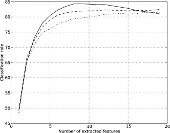
Figure 3: Classification rate in function of the number of extracted features. Continuous line corresponds to 5-NPFS, dashed line to SVM with a Gaussian kernel and dash-doted line to a linear SVM.

The mean processing time for the University of Pavia data set for several training set sizes is reported in Table III. It includes parameter optimization for SVM${}_{\text{gauss}}$ and SVM${}_{\ell_{1}}$. Note that the RFE consists in several SVM${}_{\text{gauss}}$ optimization, one for each feature removed (hence, if 3 features are removed, the mean processing time is approximately multiply by 3). It can be seen that the 5-NPFS method is a little influenced by the size of the training set: what is important is the number of (extracted) variables. For $n_{s}=50$, the processing time is slightly higher because of overload due to parallelization procedure. $n$-NPFS is the more demanding in terms of processing time and thus should be used only when the number of training samples is very limited. Finally, it is important to underline that the NPFS is implemented in Python while SVM used a state of the art implementation in C++ [25].

TABLE III: Mean processing time in second in function of the number of samples per class for the University of Pavia data set. 20 repetitions have been done on laptop with 8Gb of RAM and Intel(R) Core(TM) i7-3667U CPU @ 2.00GHz processor.

$n_{s}$	50	100	200	400
SVM${}_{\text{gauss}}$	11	40	140	505
SVM${}_{\ell_{1}}$	52	115	234	498
$n$-NPFS	242	310	472	883
5-NPFS	35	31	29	43

From these experiments, and from a practical viewpoint, NPFS is a good compromise between high classification accuracy and sparse modeling.

III-D Discussion

The extracted channels by 5-NPFS and $n$-NPFS were compared for one training set of the University of Pavia data set: two channels were the same for both methods, 780nm and 776nm; two channels were very close, 555nm and 847nm for 5-NPFS and 551nm and 855nm for $n$-NPFS; one channel was close, 521nm for 5-NPFS and 501nm for $n$-NPFS. The other channel selected by $n$-NPFS is 772nm. If the process is repeated, the result is terms of selected features by $n$-NPFS and 5-NPFS is similar: on average 35% of the selected features are identical (not necessarily the first ones) and the others selected features are close in terms of wavelength.

The influence of the parameter delta has been investigated on the University of Pavia data set. 20 repetitions have been done with $n_{c}=50$ for several values of delta. Results are reported on figure 4. From the figure, it can be seen that when delta is set to a value larger than approximately 1%, the algorithm stops too early and the number of selected features is too low to perform well. Conversely, setting delta to a small value does not change the classification rate, a plateau being reached for delta lower than 0.5%. In fact, because of the “Hughes phenomenon”, adding spectral features to the GMM will first lead to an increase of the classification rate but then (after a possible plateau) the classification rate will decrease, i.e., the improvement after two iterations of the algorithm will be negative.

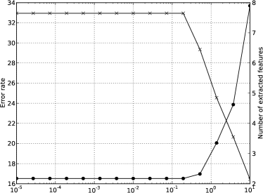
Figure 4: The dotted line and the crossed line represent the mean error rate and the mean number of selected features, respectively, as a function of delta. The simulation was done on the University of Pavia data set, with $n_{c}=50$ and for the 5-NPFS algorithm.

Figure 5 presents the most selected features for the University of Pavia data set. 1000 random repetitions have been done with $n_{c}$=200 and the features shaded in the figure have been selected at least 10% times (i.e., 100 times over 1000) using 5-NPFS. Five spectral domains can be identified, two from the visible range and three from the near infrared range. In particular, it can be seen that spectral channels from the red-edge part are selected. The width of the spectral domain indicates the variability of the selection. The high correlation between adjacent spectral bands makes the variable selection “unstable”, e.g., for a given training set, the channel $t$ would be selected but for another randomly selected training set it might be the channel $t+1$ or $t-1$. It is clearly a limitation of the proposed approach.

To conclude this discussion, similar spectral channels are extracted with $n$-NPFS and 5-NPFS, while the latter is much times faster. Hence, $n$-NPFS should be only used when very limited number of samples is available. A certain variability is observed in the selection of the spectral channels due to the high correlation of adjacent spectral channels and the step-wise nature of the method.

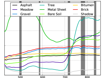
Figure 5: Most selected spectral domain for the University of Pavia data set. Gray bars correspond to the most selected parts of the spectral domain. Horizontal axis corresponds to the wavelength (in nanometers). The mean value of each class is represented in continuous colored lines.

IV Conclusion

A nonlinear parsimonious feature selection algorithm for the classification of hyperspectral images and the selection of spectral variables has been presented. Using a Gaussian mixture model classifier, spectral variables are extracted iteratively based on the cross-validation estimate of the classification rate. An efficient implementation is proposed that takes into account some properties of Gaussian mixture model: a fast update of the model parameters and a fast access to the sub-models. Experimental results show that the proposed method is able to select few relevant features, and outperform standard SVM-based sparse algorithms while reaching similar classification rates to those obtained with SVM. Furthermore, in comparison to SVM based feature selection algorithm, multiclass problem is handled by the GMM making the interpretation of the extracted channels easier.

More investigation are needed to fully understand which features are extracted, since the method is purely statistical. If the red-edge has been identified, the others extracted features are not clearly interpretable. Moreover, small variability has been observed due to the high correlation between adjacent bands and the step-wise procedure. To overcome this limitation, a continuous interval selection strategy, as in [12], will be investigated. Also, a steepest-ascent search strategy could be used to make the final solution more stable.

The python code of the algorithm is available freely for download: https://github.com/mfauvel/FFFS.

V Acknowledgment

The authors would like to thank Professor P. Gamba, University of Pavia, for providing the University of Pavia data set and Professor J.A. Benediktsson, University of Iceland, for providing the Hekla data set. They would like also to thank the reviewers for their many helpful comments.

References

- [1] L. O. Jimenez and D. A. Landgrebe, “Supervised classification in high-dimensional space: geometrical, statistical, and asymptotical properties of multivariate data,” Systems, Man, and Cybernetics, Part C: Applications and Reviews, IEEE Transactions on, vol. 28, no. 1, pp. 39 –54, feb 1998.
- [2] D. L. Donoho, “High-dimensional data analysis: the curses and blessing of dimensionality,” in AMS Mathematical challenges of the 21st century, 2000.
- [3] G. F. Hughes, “On the mean accuracy of statistical pattern recognizers,” IEEE Trans. Inf. Theory, vol. IT-14, pp. 55–63, January 1968.
- [4] M. Fauvel, Y. Tarabalka, J. A. Benediktsson, J. Chanussot, and J. Tilton, “Advances in Spectral-Spatial Classification of Hyperspectral Images,” Proceedings of the IEEE, vol. 101, no. 3, pp. 652–675, Mar. 2013.
- [5] C. J. C. Burges, “Dimension reduction: A guided tour,” Foundations and Trends in Machine Learning, vol. 2, no. 4, pp. 275–365, 2010.
- [6] G. Camps-Valls and L. Bruzzone, Eds., Kernel Methods for Remote Sensing Data Analysis, Wiley, 2009.
- [7] A. Cheriyadat and L. M. Bruce, “Why principal component analysis is not an appropriate feature extraction method for hyperspectral data,” in Geoscience and Remote Sensing Symposium, 2003. Proceedings, July 2003, vol. 6, pp. 3420–3422 vol.6.
- [8] A. Villa, J. A. Benediktsson, J. Chanussot, and C. Jutten, “Hyperspectral image classification with independent component discriminant analysis,” IEEE Trans. Geosci. Remote Sens., vol. 49, no. 12, pp. 4865–4876, Dec 2011.
- [9] M. Fauvel, J. A. Benediktsson, J. Chanussot, and J. R. Sveinsson, “Spectral and Spatial Classification of Hyperspectral Data Using SVMs and Morphological Profiles,” IEEE Trans. Geosci. Remote Sens., vol. 46, no. 11 - part 2, pp. 3804–3814, Oct. 2008.
- [10] F.E. Fassnacht, C. Neumann, M. Forster, H. Buddenbaum, A. Ghosh, A. Clasen, P.K. Joshi, and B. Koch, “Comparison of feature reduction algorithms for classifying tree species with hyperspectral data on three central european test sites,” Selected Topics in Applied Earth Observations and Remote Sensing, IEEE Journal of, vol. 7, no. 6, pp. 2547–2561, June 2014.
- [11] M. Lothode, V. Carrere, and R. Marion, “Identifying industrial processes through vnir-swir reflectance spectroscopy of their waste materials,” in Geoscience and Remote Sensing Symposium (IGARSS), 2014 IEEE International, July 2014, pp. 3288–3291.
- [12] S.B. Serpico and G. Moser, “Extraction of spectral channels from hyperspectral images for classification purposes,” IEEE Trans. Geosci. Remote Sens., vol. 45, no. 2, pp. 484–495, Feb 2007.
- [13] C.-I Chang, Hyperspectral Data Exploitation: Theory and Applications, Wiley, 2007.
- [14] S.B. Serpico and L. Bruzzone, “A new search algorithm for feature selection in hyperspectral remote sensing images,” Geoscience and Remote Sensing, IEEE Transactions on, vol. 39, no. 7, pp. 1360–1367, Jul 2001.
- [15] L. Bruzzone and C. Persello, “A novel approach to the selection of spatially invariant features for the classification of hyperspectral images with improved generalization capability,” Geoscience and Remote Sensing, IEEE Transactions on, vol. 47, no. 9, pp. 3180–3191, Sept 2009.
- [16] A.C. Jensen and R. Solberg, “Fast hyperspectral feature reduction using piecewise constant function approximations,” Geoscience and Remote Sensing Letters, IEEE, vol. 4, no. 4, pp. 547–551, Oct 2007.
- [17] A. Le Bris, N. Chehata, X. Briottet, and N. Paparoditis, “Use intermediate results of wrapper band selection methods : a first stpe toward the optimisation of spectral configuration for land cover classifications,” in Proc. of the IEEE WHISPERS’14, 2014.
- [18] D. Tuia, F. Pacifici, M. Kanevski, and W. J. Emery, “Classification of very high spatial resolution imagery using mathematical morphology and support vector machines,” Geoscience and Remote Sensing, IEEE Transactions on, vol. 47, no. 11, pp. 3866–3879, 2009.
- [19] D. Tuia, M. Volpi, M. Dalla Mura, A. Rakotomamonjy, and R. Flamary, “Automatic feature learning for spatio-spectral image classification with sparse SVM,” IEEE Trans. Geosci. Remote Sens., vol. PP, no. 99, pp. 1–13, 2014.
- [20] G. Camps-Valls, J. Mooij, and Bernhard Scholkopf, “Remote sensing feature selection by kernel dependence measures,” Geoscience and Remote Sensing Letters, IEEE, vol. 7, no. 3, pp. 587–591, July 2010.
- [21] F. Ferraty, P. Hall, and P. Vieu, “Most-predictive design points for functional data predictors,” Biometrika, vol. 97, no. 4, pp. 807–824, 2010.
- [22] T. Hastie, R. Tibshirani, and J. H. Friedman, The Elements of Statistical Learning: Data Mining, Inference, and Prediction, Springer series in statistics. Springer, 2001.
- [23] C. E. Rasmussen and C. K. I. Williams, Gaussian Processes for Machine Learning (Adaptive Computation and Machine Learning), The MIT Press, 2005.
- [24] R.-E. Fan, K.-W. Chang, C.-J. Hsieh, X.-R. Wang, and C.-J. Lin, “LIBLINEAR: A library for large linear classification,” Journal of Machine Learning Research, vol. 9, pp. 1871–1874, 2008.
- [25] Chih-C. Chang and C.-J. Lin, “LIBSVM: A library for support vector machines,” ACM Transactions on Intelligent Systems and Technology, vol. 2, pp. 27:1–27:27, 2011, Software available at http://www.csie.ntu.edu.tw/~cjlin/libsvm.