Stabilization of three-wave vortex beams in the waveguide

Abstract

We consider two-dimensional (2D) localized vortical modes in the three-wave system with the quadratic ($\chi^{(2)}$) nonlinearity, alias nondegenerate second-harmonic-generating system, guided by the isotropic harmonic-oscillator (HO) (alias parabolic) confining potential. In addition to the straightforward realization in optics, the system models mixed atomic-molecular Bose-Einstein condensates (BECs). The main issue is stability of the vortex modes, which is investigated through computation of instability growth rates for eigenmodes of small perturbations, and by means of direct simulations. The threshold of parametric instability for single-color beams, represented solely by the second harmonic (SH) with zero vorticity, is found in an analytical form with the help of the variational approximation (VA). Trapped states with vorticities $\left(+1,-1,0\right)$ in the two fundamental-frequency (FF) components and the SH one [the so-called hidden-vorticity (HV) modes] are completely unstable. Also unstable are semi-vortices (SVs), with component vorticities $\left(1,0,1\right)$. However, full vortices, with charges $\left(1,1,2\right)$, have a well-defined stability region. Unstable full vortices feature regions of robust dynamical behavior, where they periodically split and recombine, keeping their vortical content.

Keywords: vortex, second-harmonic-generation, parametric instability, azimutal instability, quadratic nonlinearity
PACS numbers: 05.45.Yv, 42.65.Tg, 42.65.Lm

1 Introduction

The fundamental significance of the quadratic ($\chi^{(2)}$) nonlinearity in optics, including its use for the creation of solitons, is well known [1]-[4], [5]. In particular, the $\chi^{(2)}$ nonlinearity opens the way to the making of two- and three-dimensional (2D and 3D) solitons, because, unlike the Kerr (cubic) terms, the quadratic ones, which couple the fundamental-frequency (FF) and second-harmonic (SH) components of the optical fields, do not give rise to the collapse in the two- and three-dimensional (2D and 3D) space [8], which is a severe problem for multidimensional solitons in Kerr media [4]. Stable (2+1)D beams propagating in quadratically nonlinear optical media have been demonstrated in the experiment [9], and stable spatiotemporal “light bullets” have been predicted in these media too [10]. In the experiment, fully self-trapped “bullets” have not been reported yet, the closest result being a spatiotemporal soliton self-trapped in the longitudinal and one transverse directions, while the confinement in the additional transverse direction was imposed by the guiding structure [11, 12].

A challenging issue for the (2+1)D setting is the search for conditions securing the stability of vortical solitons. In contrast to their fundamental counterparts, vortex solitons supported by the quadratic instability in the free space are always unstable against azimuthal perturbations, which tend to split the vortex into a set of separating fragments. For the degenerate quadratic system, with a single FF component, the splitting instability was predicted theoretically [14]-[17] and demonstrated in the experiment [18]. The same instability occurs in the framework of the full three-wave system, which includes two distinct FF components, which represent mutually orthogonal polarizations of light [19, 20].

Vortex solitons are also known as solutions of the 2D nonlinear Schrödinger (NLS) equation with the self-focusing cubic term [21]. They too are  subject to the azimuthal instability, which is actually stronger than the collapse instability driven by the cubic nonlinearity [4]. The 2D NLS equation models not only light beams in bulk media with the Kerr nonlinearity, but also the mean-field dynamics of atomic Bose-Einstein condensates (BECs), trapped in the form of “pancakes” by the confining potential [22]; in the latter case, the NLS equation is usually called the Gross-Pitaevskii (GP) equation. In the context of the NLS/GP equation, a practically relevant solution of the instability problem was elaborated: both fundamental and vortical solitons, with topological charge $m=0$ and $1$, respectively, can be stabilized by 2D harmonic-oscillator (HO) confining potentials. It is well known [23]-[29] that the HO potential renders the fundamental solitons stable, against small perturbations, in the entire region of their existence. The vortices with $m=1$, trapped by the same potential, are stabilized in $\simeq 33\%$ of their existence region (in terms of their norm). Additionally, an adjacent region of width $\simeq 10\%$ supports a robust dynamical regime featuring periodic splitting and recombination of the vortices, which keep their topological charge [27]. As concerns the BEC realization, stabilization of self-trapped semi-vortex modes in the free 2D space was recently demonstrated in a two-component system with the Kerr nonlinearity and linear spin-orbit coupling between the components [30].

The effective 2D trapping potential can be also realized in optical waveguides, in the form of the respective profile of the transverse modulation of the local refractive index [5]. This circumstance suggests a natural possibility for the stabilization of (2+1)D vortex solitons in the $\chi^{(2)}$ medium by means of the radial HO potential. For the degenerate (two-wave) $\chi^{(2)}$ system, alias the Type-I second-harmonic-generating interaction [1]-[3], this possibility was demonstrated in Ref. [31], and then extended for 3D spatiotemporal vortex solitons in Ref. [32]. The subject of the present work is to investigate this stabilization mechanism for the nondegenerate three-wave system, with the Type-II quadratic interaction, where the results demonstrate essentially new features in comparison with the degenerate model.

A feasible approach to the making of the optical medium combining a nearly-parabolic profile of the refractive index and $\chi^{(2)}$ nonlinearity is the use of a 2D photonic crystal, which can be readily designed to emulate the required index profile, while the quadratic nonlinearity may be provided by poled material filling voids of the photonic-crystal matrix [6], [7]. In fact, the effective radial potential provides for sufficiently strong localization of the trapped modes, therefore the exact parabolic shape of the radial profile is not crucially important [31].

Essentially the same system of GP equations for atomic and molecular wave functions models the BEC in atomic-molecular mixtures [33]-[36]. In that case, two different components of the atomic wave function pertain to two different atomic states of the same species, while the quadratic nonlinearity accounts for reactions of the merger of two atoms into a molecule, and splitting of the molecules due to collisions with free atoms. Accordingly, the predicted mechanism of the stabilization of three-component vortex solitons trapped in the HO potential can also be realized in the BEC mixture.

The paper is organized as follows. The model, based on the system of three propagation equation coupled by the $\chi^{(2)}$ terms, is introduced in Section II. In Section III, we introduce four types of three-wave modes considered in this work: the SH-only (single-color) one, with zero FF components; modes with the hidden vorticity (HV, which means opposite vorticities, $S=\pm 1$, in the two FF components, and $S=0$ in the SH component); semi-vortices, with $S=0$ in one FF component and $S=1$ in the other one and in the SH wave (cf. the above-mentioned semi-vortices in the two-component system with the cubic nonlinearity and linear spin-orbit coupling between the components [30]); and, finally, full vortices, with $S=1$ in both FF components, and $S=2$ in the SH. In Section IV we report simple but nontrivial analytical results, which predict the threshold of the parametric instability for the fundamental and vortical single-color states by means of the variational approximation (VA). In Section V we formulate the eigenvalue problem for small perturbations around stationary solutions, which determines their stability. The numerical results for modes of all the types are reported in Section VI. First, we identify the stability threshold for the fundamental and vortical single-color trapped modes, and compare these results with the above-mentioned analytical predictions provided by the VA. Next, the results are summarized for the HV and SV modes, which are found to be unstable. Finally, the stability region is presented for the most general three-wave states, with vorticities $1$ in both FF components and $2$ in the SH. In addition, unstable vortices may exist in a quasi-stable dynamical regime, in the form of periodic splitting and recombination of the semi-vortex. The paper is concluded by Section VII.

2 The model

The copropagation of two components of the FF wave, with amplitudes $u\left(x,y,z\right)$ and $v\left(x,y,z\right)$, and the SH wave, with amplitude $w\left(x,z\right)$, in the bulk $\chi^{(2)}$ waveguide obeys the system of three coupled equations written here in the normalized form [2, 3]:

$$iu_{z} = -\frac{1}{2}\nabla^{2}u+v^{\ast}w+\frac{1}{2}\Omega^{2}r^{2}u+Qu,$$ (1)

$$iv_{z} = -\frac{1}{2}\nabla^{2}v+u^{\ast}w+\frac{1}{2}\Omega^{2}r^{2}v-Qv,$$ (2)

$$2iw_{z} = -\frac{1}{2}\nabla^{2}w-qw+uv+2\Omega^{2}r^{2}w,$$ (3)

where $\nabla^{2}\equiv\partial^{2}/\partial x^{2}+\partial^{2}/\partial y^{2}$ is the transverse diffraction operator, the asterisk stands for the complex conjugate, $Q$ is the birefringence coefficient, $q$ is the FF-SH phase mismatch, and $\Omega^{2}$ the strength of the HO trapping potential. In the most general case, stationary vortex solutions of this system, with two independent FF propagation constants $k_{u}$ and $k_{v}$, can be looked for as

$$\left\{u,v\right\} = \left\{U_{0}(r)e^{iS_{u}\theta+ik_{u}z},V_{0}(r)e^{iS_{v}\theta+ik_{v}z}\right\},$$ (4)

$$w = W_{0}(r)e^{i\left(S_{u}+S_{v}\right)+i\left(k_{u}+k_{v}\right)z},$$ (5)

where $S_{u}$ and $S_{v}$ are integer vorticities of the two FF components, and $U_{0}(r)$, $V_{0}(r)$, and $W_{0}(r)$ are real radial functions with asymptotic forms

$$\left\{U_{0}(r),V_{0}(r),W_{0}(r)\right\}\sim r^{\left\{\left|S_{u}\right|,\left|S_{v}\right|,\left|S_{u}+S_{v}\right|\right\}}~{}\ \mathrm{at}~{}~{}r\rightarrow 0,$$

$$\left\{U_{0}(r),V_{0}(r)\right\}\sim\exp\left(-\frac{\Omega}{2}r^{2}\right),~{}W_{0}(r)\sim\exp\left(-\Omega r^{2}\right)\ \mathrm{at}~{}~{}r\rightarrow\infty.$$ (6)

The exact equality of the propagation constant and vorticity of the SH component in Eqs. (4) and (5) to sums of the same constants of the FF components is imposed by the coherent coupling between the FF and SH components in Eqs. (1), (2), and (3).

In this work, the analysis is carried out, chiefly, for $Q=0$, in which case the symmetry between the two FF components suggests to consider three-wave states with $k_{u}=k_{v}$. For $Q\neq 0$, rescaling of Eqs. (1)-(2) makes it possible to fix $Q=1$. Families of three-wave vortices with $Q=1$ are considered too, at the end of the paper.

Equations (1)-(3) can be derived from the Lagrangian,

$$L=\int\int\left\{\frac{i}{2}\left[\left(uu_{z}^{\ast}-u^{\ast}u_{z}\right)+i\left(vv_{z}^{\ast}-v^{\ast}v_{z}\right)+2\left(ww_{z}^{\ast}-w^{\ast}w_{z}\right)\right]\right\}dxdy-H,$$ (7)

where the Hamiltonian is

$$H = \int\int\left[\frac{1}{2}\left(\left|\nabla u\right|^{2}+\left|\nabla u\right|^{2}+\left|\nabla w\right|^{2}\right)+\frac{1}{2}\Omega^{2}r^{2}\left(|u|^{2}+|v|^{2}+4|w|^{2}\right)\right.$$ (8)

$$\left.+Q\left(|u|^{2}-|v|^{2}\right)-q|w|^{2}+\left(uvw^{\ast}+u^{\ast}v^{\ast}w\right)\right]dxdy.$$

The Hamiltonian is the dynamical invariant of Eqs. (1)-(3), along with the total power (field norm),

$$N=\int\int\left(|u|^{2}+|v|^{2}+4|w|^{2}\right)dxdy\equiv N_{u}+N_{v}+N_{w},$$ (9)

and the total angular momentum,

$$M=i\int\int\left[u^{\ast}\left(yu_{x}-xu_{y}\right)+v^{\ast}\left(yv_{x}-xv_{y}\right)+2w^{\ast}\left(yw_{x}-xw_{y}\right)\right]dxdy,$$ (10)

which is a real integral quantity, even if it formally seems complex. (it can be checked by means of the integration by parts that the $M^{*}\equiv M$).

3 Stationary solutions

3.1 Single-color (second-harmonic) states

The simplest stationary state in the present model is the one with unexcited FF components, i.e., $U_{0}=V_{0}=0$ in Eq. (4) and $W_{0}(r)$ from Eq. (5) obeying the linear equation, which follows from Eq. (3):

$$\left(-4k+q\right)W_{0}=-\frac{1}{2}\left(W_{0}^{\prime\prime}+\frac{1}{r}W_{0}^{\prime}-\frac{S_{w}^{2}}{r^{2}}\right)+2\Omega^{2}r^{2}W_{0},$$ (11)

where $S_{w}$ replaces $\left(S_{u}+S_{v}\right)$, see Eq. (5). This equation is tantamount to the radial Schrödinger equation for 2D quantum-mechanical states with azimuthal quantum number $S$ in the HO potential. The respective solutions to Eq. (11) are

$$W_{0}=Br^{|S_{w}|}\exp\left(-\Omega r^{2}\right),$$ (12)

$$k=-\Omega\left(1+|S_{w}|\right)/2+q/4,$$ (13)

where $B$ is an arbitrary constant. The norm (9) of this state is

$$N_{\mathrm{SH}}=\frac{4\pi\left|S_{w}\right|!}{\left(2\Omega\right)^{1+\left|S_{w}\right|}}B^{2}.$$ (14)

3.2 Hidden-vorticity (HV) states

Solutions for 2D HV modes are defined by the vorticity set $\left(S_{u},S_{v},S_{w}\equiv S_{u}+S_{v}\right)=\left(+1,-1,0\right)$ of the three components in Eqs. (4) and (5). Accordingly, the solutions are looked for as

$$\left\{u,v\right\}=\left\{U_{0}(r)e^{iS\theta},V_{0}(r)e^{-iS\theta}\right\}e^{ikz},$$ (15)

$$w=W_{0}(r)e^{2ikz},$$ (16)

where real functions $U_{0},$ $V_{0},$ and $W_{0}$ satisfy the following radial equations (where the birefringence terms are kept, for the time being):

$$-kU_{0} = -\frac{1}{2}\left(U_{0}^{\prime\prime}+\frac{1}{r}U_{0}^{\prime}-\frac{S^{2}}{r^{2}}U_{0}\right)+V_{0}W_{0}+\frac{1}{2}\Omega^{2}r^{2}U_{0}+QU_{0},$$ (17)

$$-kV_{0} = -\frac{1}{2}\left(V_{0}^{\prime\prime}+\frac{1}{r}V_{0}^{\prime}-\frac{S^{2}}{r^{2}}V_{0}\right)+U_{0}W_{0}+\frac{1}{2}\Omega^{2}r^{2}V_{0}-QV_{0},$$ (18)

$$-4kW_{0} = -\frac{1}{2}\left(W_{0}^{\prime\prime}+\frac{1}{r}W_{0}^{\prime}\right)-qW_{0}+U_{0}V_{0}+2\Omega^{2}r^{2}W_{0}.$$ (19)

Previously, the HV concept was realized for the three-wave $\chi^{(2)}$ system in the free space [37], as well as for various systems of coupled continuous [38]-[41] and discrete [42, 43] NLS/GP equations with the cubic nonlinearity, including the system supported by the HO trapping potential [41]. In work [44], it was demonstrated that the HV essentially suppresses the modulational instability of 2D ring solitons in a two-component system with saturable nonlinearity, in comparison with their counterparts carrying explicit vorticity. However, trapped vortical modes with HV were not previously studied in three-wave systems.

3.3 Semi-vortices

The other type of the vortical mode, with zero vorticity in one FF component (hence they are called semi-vortices, as said above), is defined by the set of $\left(S_{u},S_{v},S_{w}\right)=\left(1,0,1\right)$, i.e., solution ansatz (4), (5) reduces to

$$\left\{u,v\right\} = \left\{U_{0}(r)e^{i\theta+ik_{1}z},V_{0}(r)e^{ik_{2}z}\right\},$$ (20)

$$w = W_{0}(r)e^{i\theta+i\left(k_{1}+k_{2}\right)z},$$ (21)

where the real radial amplitudes obey the following equations, cf. Eqs. (17), (18), (19):

$$-k_{1}U_{0} = -\frac{1}{2}\left(U_{0}^{\prime\prime}+\frac{1}{r}U_{0}^{\prime}-\frac{1}{r^{2}}U_{0}\right)+V_{0}W_{0}+\frac{1}{2}\Omega^{2}r^{2}U_{0}+QU_{0},$$

$$-k_{2}V_{0} = -\frac{1}{2}\left(V_{0}^{\prime\prime}+\frac{1}{r}V_{0}^{\prime}\right)+U_{0}W_{0}+\frac{1}{2}\Omega^{2}r^{2}V_{0}-QV_{0},$$ (22)

$$-2\left(k_{1}+k_{2}\right)W_{0} = -\frac{1}{2}\left(W_{0}^{\prime\prime}+\frac{1}{r}W_{0}^{\prime}-\frac{1}{r^{2}}W_{0}\right)-qW_{0}+U_{0}V_{0}+2\Omega^{2}r^{2}W_{0}.$$

In the limit of small amplitudes, solutions of the linearized version of Eqs. (22) can be found in the form of

$$U_{0} = U_{0}^{(0)}r\exp\left(-\Omega r^{2}/2\right),$$

$$V_{0} = W_{0}^{(0)}\exp\left(-\Omega r^{2}/2\right),$$ (23)

$$W_{0} = W_{0}^{(0)}r\exp\left(-\Omega r^{2}\right),$$

where the propagation constant must satisfy, respectively, the following relations for the components $U,V,W$:

$$k_{1} = -2\Omega-Q,$$

$$k_{2} = -\Omega+Q,$$ (24)

$$k_{1}+k_{2} = -2\Omega+q/2,$$

From Eqs. (24) it follows that, in the small-amplitude limit, the semi-vortex mode exists at the single value of the mismatch, $q=-2\Omega$. Below, it is shown that solutions for nonlinear semi-vortex modes lift this constraint.

3.4 Full vortices

In fact, the HV modes and semi-vortices are shown below to be completely unstable (modes of the latter type may be replaced by robust dynamical states which keep the same vortical structure). A stationary topological state which features a well-defined stability region is the full vortex, with the set of $\left(S_{u},S_{v},S_{w}\right)=\left(1,1,2\right)$ in Eqs. (4) and (5). The respective system of stationary equations is [cf. Eqs. (17)-(19) and (22)]:

$$-k_{1}U_{0} = -\frac{1}{2}\left(U_{0}^{\prime\prime}+\frac{1}{r}U_{0}^{\prime}-\frac{1}{r^{2}}U_{0}\right)+V_{0}W_{0}+\frac{1}{2}\Omega^{2}r^{2}U_{0}+QU_{0},$$

$$-k_{2}V_{0} = -\frac{1}{2}\left(V_{0}^{\prime\prime}+\frac{1}{r}V_{0}^{\prime}-\frac{1}{r^{2}}V_{0}\right)+U_{0}W_{0}+\frac{1}{2}\Omega^{2}r^{2}V_{0}-QV_{0},$$ (25)

$$-2\left(k_{1}+k_{2}\right)W_{0} = -\frac{1}{2}\left(W_{0}^{\prime\prime}+\frac{1}{r}W_{0}^{\prime}-\frac{4}{r^{2}}W_{0}\right)-qW_{0}+U_{0}V_{0}+2\Omega^{2}r^{2}W_{0}.$$

4 The variational approximation (VA) for the onset of the parametric instability of the single-color modes

The VA is a natural approach for predicting the shape of nonlinear modes, including vortical ones supported by the $\chi^{(2)}$ nonlinearity [31, 30]. In the present context, the VA can be used for the prediction of the instability threshold of the trapped single-color (SH-only) states (the VA may be developed for other situations too, but it then turns out to be rather cumbersome).

For this purpose, it is necessary to consider a perturbed version of the single-color stationary state, which includes the FF components too. In particular, in the case of zero vorticity of the SH component and vorticities $\pm S$ of the FF perturbations, the Lagrangian of the respective stationary equations (17)-(19) can be reduced to its radial part:

$$L_{\mathrm{rad}}=\int_{0}^{\infty}rdr\left\{\frac{1}{2}\left[\left(\frac{dU_{0}}{dr}\right)^{2}+\left(\frac{dV_{0}}{dr}\right)^{2}+\left(\frac{dW_{0}}{dr}\right)^{2}+\frac{S^{2}}{r^{2}}\left(U_{0}^{2}+V_{0}^{2}\right)\right]\right.$$

$$+k\left(U_{0}^{2}+V_{0}^{2}+4W_{0}^{2}\right)+\frac{1}{2}\Omega^{2}r^{2}\left(U_{0}^{2}+V_{0}^{2}+4W_{0}^{2}\right)+Q\left(U_{0}^{2}-V_{0}^{2}\right)-qW_{0}^{2}$$

$$\left.+2U_{0}V_{0}W_{0}\right\}.$$ (26)

To develop the VA, the simplest Gaussian ansatz may be adopted, assuming equal amplitudes ($A$) and widths of fields $U_{0}$ and $V_{0}$:

$$U_{0}(r)=V_{0}(r)=Ar^{S}\exp\left(-\Omega r^{2}/2\right),W_{0}(r)=B\exp\left(-\Omega r^{2}\right)$$ (27)

($S\geq 0$ is defined here). The symmetry between the FF components implies that we should set $Q=0$, otherwise the symmetry will be broken by the birefringence. Setting $Q=0$ limits the consideration to a particular case of the generic three-wave system, but even this particular case is a nontrivial one, as it has no counterpart in the usually considered degenerate two-wave system, in which the VA was applied before to the description of trapped vortices [31]. The widths of all the components in ansatz (27) are not treated as variational parameters, but are rather taken as per wave functions of states trapped in the 2D harmonic-oscillator potential, cf. Eq. (12).

The objective of the use of the VA in the present context is to predict a point at which a solution with an infinitely small $A$ appears, against the background of the fundamental single-color (SH-only) state, given by Eqs. (12), (13) with $S_{w}=0$ and arbitrary amplitude $B$. The appearance of this mode signals the onset of the parametric instability of the latter state [31]. The substitution of ansatz (27) into radial Lagrangian (26) yields the following reduced Lagrangian, in which we drop terms that produce no contribution in the subsequent analysis:

$$L_{\mathrm{rad}}=S!\frac{A^{2}}{\Omega^{S}}\left[1+S+\frac{k}{\Omega}+2^{-\left(1+S\right)}\frac{B}{\Omega}\right].$$ (28)

This Lagrangian gives rise to the Euler-Lagrange equation, $\partial L_{\mathrm{rad}}/\partial\left(A^{2}\right)=0$. The parametric-instability threshold, corresponding to the emergence of the solution with an infinitesimal $A^{2}>0$, corresponds to setting $A^{2}=0$ in the resulting equation:

$$B=-2^{1+S}\left[\left(1+S\right)\Omega+k\right]=-2^{1+S}\left[\left(\frac{1}{2}+S\right)\Omega+\frac{q}{4}\right],$$ (29)

where expression (13) was substituted for $k$. The respective critical total power (norm) of the trapped single-color state is given by Eq. (14),

$$N_{c}=2^{1+2S}\frac{\pi}{\Omega}\left[\left(1+2S\right)\Omega+\frac{q}{2}\right]^{2}.$$ (30)

Thus, the fundamental single-color state is stable at $N<N_{c}$, and unstable at $N>N_{c}$.

Note that, as it follows from Eq. (30), the parametric instability of the zero-vorticity single-color state is dominated by the vortical FF perturbations with $S=1$ (i.e., $S=1$ give rise to $N_{c}$ lower than its counterpart produced by the zero-vorticity perturbations, with $S=0$) in an interval of negative values of the mismatch, $\left(14/3\right)\Omega<-q<10\Omega$.

It is also relevant to develop a similar analysis for the onset of the parametric instability of the vortical single-color trapped state with even vorticity $S_{w}>0$, for which $W_{0}(r)=Br^{S_{w}}\exp\left(-\Omega r^{2}\right)$, cf. Eq. (12), and $S$ is replaced by $S_{w}/2$ in the FF components of ansatz (27). In this case, the reduced radial Lagrangian (28) is replaced by

$$L_{\mathrm{rad}}^{\mathrm{(}S_{w}\mathrm{)}}=\left(S_{w}/2\right)!\frac{A^{2}}{\Omega^{S_{w}/2}}\left(1+\frac{S_{w}}{2}+\frac{k}{\Omega}\right)+S_{w}!\frac{A^{2}B}{\left(2\Omega\right)^{S_{w}+1}}.$$ (31)

Then, the Euler-Lagrange equation, $\partial L_{\mathrm{rad}}^{\mathrm{(}S_{w}\mathrm{)}}/\partial\left(A^{2}\right)=0$, yields the value of amplitude $B$, the substitution of which into expression (14) gives the instability threshold for the single-color vortex mode:

$$N_{c}^{(S_{w})}=2^{1+S_{w}}\frac{\left[\left(S_{w}/2\right)!\right]^{2}}{S_{w}!}\frac{\pi}{\Omega}\left(\Omega+\frac{q}{2}\right)^{2}.$$ (32)

The analytical predictions (30) and (32) produced by the VA are compared to numerical findings below, see Fig. 1.

5 Linearized equations for small perturbations

The stability of the modes under the consideration is the central issue of the present work. It is addressed via computation of eigenvalues for small perturbations. In the general case, perturbed solutions are introduced as

$$u\left(z,\mathbf{r}\right) = e^{ikz}\left[u_{0}(\mathbf{r})+\varepsilon e^{\lambda z}u_{1}(\mathbf{r})+\varepsilon e^{\lambda^{\ast}z}\tilde{u}_{1}^{\ast}(\mathbf{r})\right],$$

$$v\left(z,\mathbf{r}\right) = e^{ikz}\left[v_{0}(\mathbf{r})+\varepsilon e^{\lambda z}v_{1}(\mathbf{r})+\varepsilon e^{\lambda^{\ast}z}\tilde{v}_{1}^{\ast}(\mathbf{r})\right],$$ (33)

$$w\left(z,\mathbf{r}\right) = e^{2ikz}\left[w_{0}(\mathbf{r})+\varepsilon e^{\lambda z}w_{1}(\mathbf{r})+\varepsilon e^{\lambda^{\ast}z}\tilde{w}_{1}^{\ast}(\mathbf{r})\right],$$

where $k$ is the propagation constant of the stationary solution (assuming here that $k$ is the same for that both FF components), which is represented by (complex) functions $u_{0}(\mathbf{r}),~{}v_{0}(\mathbf{r}),$ $w_{0}(\mathbf{r})$, infinitely small $\varepsilon$ is an amplitude of the perturbation, $\lambda$ is the instability growth rate sought for, which is, generally, complex too [the instability takes place if there exists, as usual, at least single $\lambda$ with $\mathrm{Re}(\lambda)>0$], the asterisk stands for the complex conjugate, and $u_{1}(\mathbf{r}),~{}\tilde{u}_{1}(\mathbf{r}),$ $v_{1}(\mathbf{r}),~{}\tilde{v}_{1}(\mathbf{r}),$ $w_{1}(\mathbf{r}),~{}\tilde{w}_{1}(\mathbf{r})$ are components of the perturbation eigenmode, which obey the system of linearized equations:

$$\left(i\lambda-k\right)u_{1}=-\frac{1}{2}\nabla^{2}u_{1}+v_{0}^{\ast}w_{1}+w_{0}\tilde{v}_{1}+\frac{1}{2}\Omega^{2}r^{2}u_{1}+Qu_{1},$$

$$\left(-i\lambda-k\right)\tilde{u}_{1}=-\frac{1}{2}\nabla^{2}\tilde{u}_{1}+v_{0}\tilde{w}_{1}+w_{0}^{\ast}v_{1}+\frac{1}{2}\Omega^{2}r^{2}\tilde{u}_{1}+Q\tilde{u}_{1},$$

$$\left(i\lambda-k\right)v_{1}=-\frac{1}{2}\nabla^{2}v_{1}+u_{0}^{\ast}w_{1}+w_{0}\tilde{u}_{1}+\frac{1}{2}\Omega^{2}r^{2}v_{1}-Qv_{1},$$

$$\left(-i\lambda-k\right)\tilde{v}_{1}=-\frac{1}{2}\nabla^{2}\tilde{v}_{1}+u_{0}\tilde{w}_{1}+w_{0}^{\ast}u_{1}+\frac{1}{2}\Omega^{2}r^{2}\tilde{v}_{1}-Q\tilde{v}_{1},$$

$$\left(2i\lambda+q-4k\right)w_{1}=-\frac{1}{2}\nabla^{2}w_{1}+u_{0}v_{1}+v_{0}u_{1}+2\Omega^{2}r^{2}w_{1},$$

$$\left(-2i\lambda+q-4k\right)\tilde{w}_{1}=-\frac{1}{2}\nabla^{2}\tilde{w}_{1}+u_{0}^{\ast}\tilde{v}_{1}+v_{0}^{\ast}\tilde{u}_{1}+2\Omega^{2}r^{2}\tilde{w}_{1}.$$ (34)

For the unperturbed solution taken as per Eqs. (15) and (16), it is easy to see that Eqs. (34) admit self-consistent perturbation modes in the following form:

$$u_{1}(r,\theta) = U_{1}(r)e^{i\left(-S_{u}+p\right)\theta},~{}\tilde{u}_{1}(r,\theta)=\tilde{U}_{1}(r)e^{i\left(S_{u}+p\right)\theta},$$

$$v_{1}(r,\theta) = V_{1}(r)e^{i\left(-S_{v}+p\right)\theta},~{}\tilde{v}_{1}(r,\theta)=\tilde{V}_{1}(r)e^{i\left(S_{v}+p\right)\theta},$$

$$w_{1}(r,\theta) = W_{1}(r)e^{i(-S_{u}-S_{v}+p)\theta},~{}\tilde{w}_{1}(r,\theta)=\tilde{W}_{1}(r)e^{i(S_{u}+S_{v}+p)\theta},$$ (35)

where $p$ is an arbitrary integer (azimuthal index of the perturbation). The substitution of expressions (35) into Eq. (34) leads to the following eigenvalue system which should determine $\lambda$ for each integer $p$:

$$\left(i\lambda-k\right)U_{1}=-\frac{1}{2}\left(\frac{d^{2}}{dr^{2}}+\frac{1}{r}\frac{d}{dr}-\frac{\left(-S_{u}+p\right)^{2}}{r^{2}}\right)U_{1}+V_{0}(r)W_{1}+W_{0}(r)\tilde{V}_{1}$$

$$+\frac{1}{2}\Omega^{2}r^{2}U_{1}+QU_{1},$$

$$\left(-i\lambda-k\right)\tilde{U}_{1}=-\frac{1}{2}\left(\frac{d^{2}}{dr^{2}}+\frac{1}{r}\frac{d}{dr}-\frac{\left(S_{u}+p\right)^{2}}{r^{2}}\right)\tilde{U}_{1}+V_{0}(r)\tilde{W}_{1}+W_{0}(r)V_{1}$$

$$+\frac{1}{2}\Omega^{2}r^{2}\tilde{U}_{1}+Q\tilde{U}_{1},$$

$$\left(i\lambda-k\right)V_{1}=-\frac{1}{2}\left(\frac{d^{2}}{dr^{2}}+\frac{1}{r}\frac{d}{dr}-\frac{\left(-S_{v}+p\right)^{2}}{r^{2}}\right)V_{1}+U_{0}(r)W_{1}+W_{0}(r)\tilde{U}_{1}$$

$$+\frac{1}{2}\Omega^{2}r^{2}V_{1}-QV_{1},$$

$$\left(-i\lambda-k\right)\tilde{V}_{1}=-\frac{1}{2}\left(\frac{d^{2}}{dr^{2}}+\frac{1}{r}\frac{d}{dr}-\frac{\left(S_{v}+p\right)^{2}}{r^{2}}\right)\tilde{V}_{1}+U_{0}(r)\tilde{W}_{1}+W_{0}(r)U_{1}$$

$$+\frac{1}{2}\Omega^{2}r^{2}\tilde{V}_{1}-Q\tilde{V}_{1},$$

$$\left(2i\lambda+q-4k\right)W_{1}=-\frac{1}{2}\left(\frac{d^{2}}{dr^{2}}+\frac{1}{r}\frac{d}{dr}-\frac{(-S_{u}-S_{v}+p)^{2}}{r^{2}}\right)W_{1}+U_{0}(r)V_{1}$$

$$+V_{0}(r)U_{1}+2\Omega^{2}r^{2}W_{1},$$

$$\left(-2i\lambda+q-4k\right)\tilde{W}_{1}=-\frac{1}{2}\left(\frac{d^{2}}{dr^{2}}+\frac{1}{r}\frac{d}{dr}-\frac{(S_{u}+S_{v}+p)^{2}}{r^{2}}\right)\tilde{W}_{1}$$

$$+U_{0}(r)\tilde{V}_{1}+V_{0}(r)\tilde{U}_{1}+2\Omega^{2}r^{2}\tilde{W}_{1}.$$ (36)

Solutions $U_{1},\tilde{U}_{1},V_{1},\tilde{V}_{1}$ of Eqs. (36) must exponentially decay at $r\rightarrow\infty$, and behave as $r^{|p\pm S_{u,v}|}$ at $r\rightarrow 0$, and $W_{1},\tilde{W}_{1}$ must exponentially decay too at $r\rightarrow\infty$, and go as $r^{|p\pm\left(S_{u}+S_{v}\right)|}$ at $r\rightarrow 0$, cf. Eq. (6).

6 The stability of the single-color modes

First, we address the stability of the SH-only vortex, which is given by Eqs. (12) and (13), against small perturbations seeded in the FF components, which are taken as

$$u\left(z,\mathbf{r}\right) = \varepsilon e^{ikz+\lambda z}u_{1}(r)e^{ip\theta},$$

$$v\left(z,\mathbf{r}\right) = \varepsilon e^{ikz+\lambda^{\ast}z}v_{1}^{\ast}(r)e^{i\left(S_{w}-p\right)\theta},$$ (37)

according to Eqs. (33), (35). The perturbation eigenfunctions, $u_{1}(r)$ and $v_{1}(r)$, satisfy the following linearized equations, which are a particular case of Eq. (36):

$$\left(i\lambda-k-Q\right)u_{1}=-\frac{1}{2}\left(\frac{d^{2}}{dr^{2}}+\frac{1}{r}\frac{d}{dr}-\frac{P^{2}}{r^{2}}\right)u_{1}$$

$$+Br^{S_{w}}e^{-\Omega r^{2}}v_{1}+\frac{1}{2}\Omega^{2}r^{2}u_{1},$$

$$\left(-i\lambda-k+Q\right)v_{1}=-\frac{1}{2}\left(\frac{d^{2}}{dr^{2}}+\frac{1}{r}\frac{d}{dr}-\frac{\left(S_{w}-P\right)^{2}}{r^{2}}\right)v_{1}$$

$$+Br^{S_{w}}e^{-\Omega r^{2}}u_{1}+\frac{1}{2}\Omega^{2}r^{2}v_{1}.$$

The objective is to find, for given $S_{w}$, a critical (minimum) value of amplitude $B$ in solution (12), and, accordingly, the minimum value of the integral power (14), at which Eq. (6) starts to produce eigenvalues with $\mathrm{Re}(\lambda)\neq 0$, i.e., the single-color mode becomes unstable against the FF perturbations. Then, we aim to explore the evolution of unstable modes by means of direct simulations. To address these problems, we employed numerical techniques and grids similar to those used in Ref. [41] for finding the eigenvalues and running direct simulations.

The results for trapped single-color (SH-only) modes are collected in the left panel of Fig. 1, while the right panel illustrates the evolution of an unstable mode with $S_{w}=0$, in terms of the power exchange between the three components (the total power is conserved, as it should be). Here and below, numerical results are displayed for the zero birefringence ($Q=0$, unless it is specified otherwise) and trapping-potential strength $\Omega=1$.

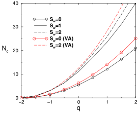
Figure 1: Left: Numerically found critical powers, $N_{c}$, of the single-color (SH-only) states, with vorticities $S_{w}=0,1,2$, beyond which the states become unstable against the excitation of the FF. For $S_{w}=0$ and $2$, the analytical results, produced by the variational approximation [see Eqs. (30) with $S=0$ and (32) with $S_{w}=2$], are displayed too. Right: The evolution of integral powers of fields $u,v$ and $w$ for a perturbed unstable state with $S_{w}=0$, $q=0$, and total power $N=7.6$. In both panels here, and in figures following below, numerical results are presented for $\Omega=1$ and $Q=0$ (zero birefringence between the FF components, except for Fig. 15).

The left panel of Fig. 1 demonstrates that the VA-predicted instability thresholds (30) and (30) approximate their numerically found counterparts well enough. In particular, the VA exactly predicts that (for $\Omega=1$ and $Q=0$), the instability threshold vanishes ($N_{c}=0$) at $q=-2$.

It is interesting to consider the (in)stability of the single-color trapped vortices with $S_{w}=1$ and other odd values of the vorticity, as the respective perturbations in the two FF components cannot be arranged symmetrically, unlike those considered above for even values of $S_{w}$. The threshold value of the norm for $S_{w}=1$ is shown in the left panel of Fig. 1, and the development of the respective instability is illustrated by Figs. (2) and (3). It can be concluded that the instability does not destroy the vorticity (topological charge) of the SH component, while the SH and FF waves exchange their angular momenta, keeping virtually equal integral powers.

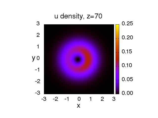
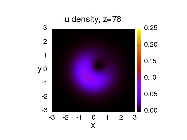
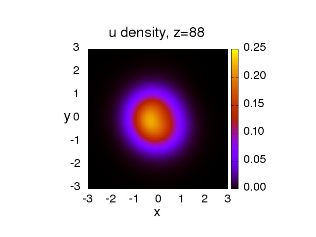
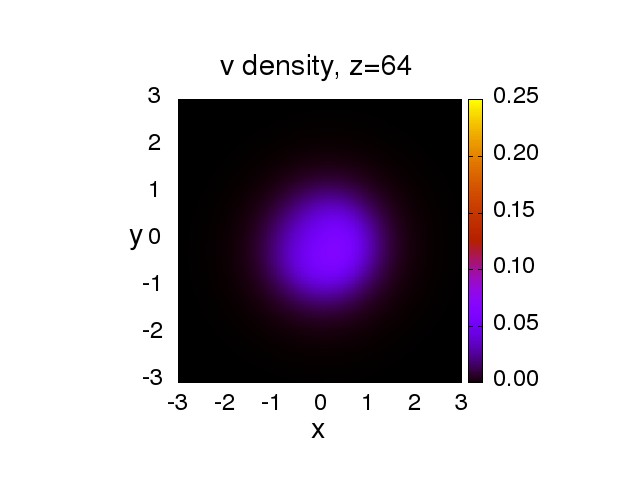
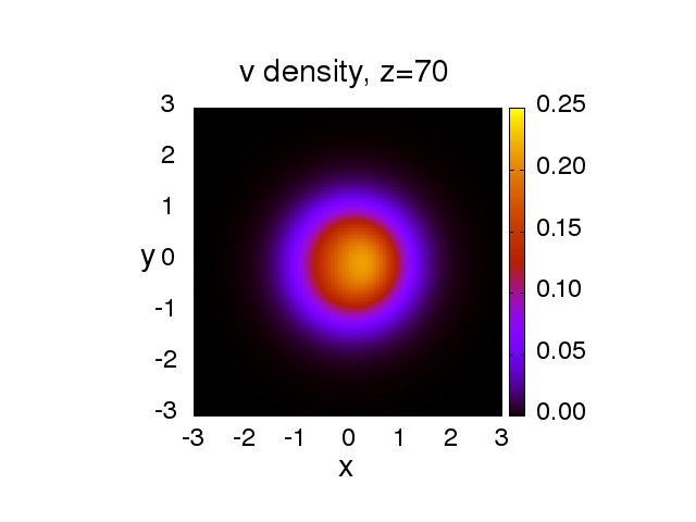
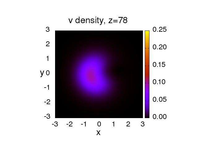
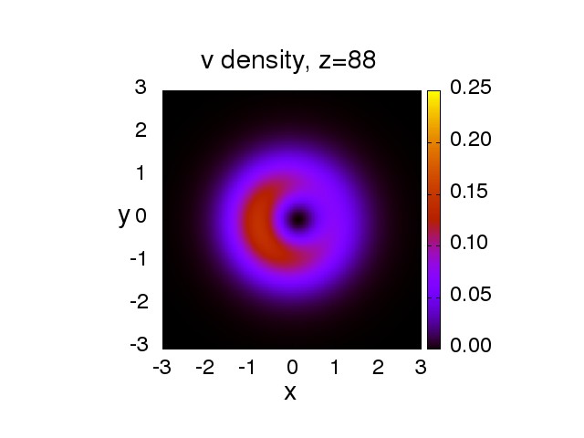
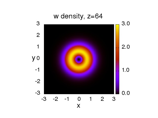
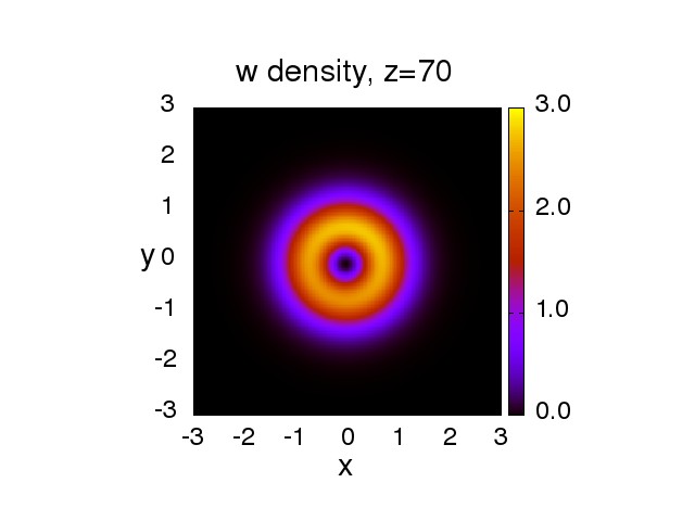
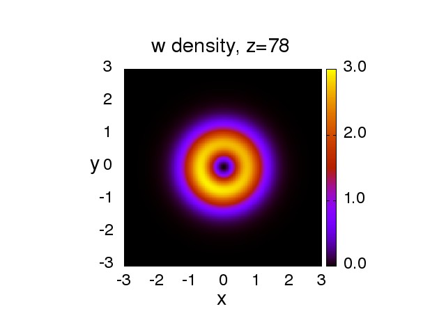
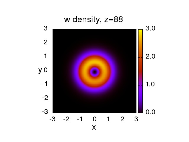
Figure 2: (Color online) Development of the instability of the single-color (SH) mode (12), for $S_{w}=1$, $Q=0$, $\Omega=1$, $B=2$, $N=4\pi$. Initial random perturbations in the FF components, $u$ and $v$, are loaded with an amplitude $<10^{-4}$. The top, middle, and bottom panels display the evolution of densities of the $u$, $v$ (FF) and $w$ (SH) fields, respectively.

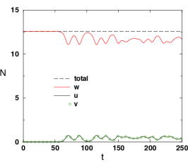
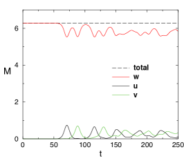
Figure 3: Overall characteristics of the instability displayed in Fig. 2. Left: The evolution of the integral powers of the FF components, $u$ and $v$. Right: The integral angular momentum of each component, see Eq. (10).

7 Numerical results for three-wave vortices

7.1 Hidden-vorticity (HV) modes with $S_{u,v,w}=\left(+1,-1,0\right)$

Families of HV states, defined as per Eqs. (15) and (16), are characterized by dependences between the propagation constant and integral powers of the two FF components and the SH one, see Eq. (9). Typical examples of such dependences, obtained from a numerical solution of Eqs. (17)-(19), are shown in the left panels of Figs. 4 and 5, respectively, for positive ($q\geq 0$) and negative ($q<0$) values of the phase mismatch.

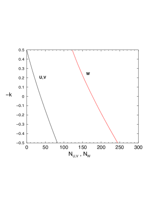
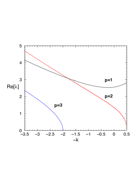
Figure 4: (Color online) Left: The propagation constant vs. the total power for the hidden-vorticity family with vorticities $S_{u,v,w}=\left(+1,-1,0\right)$, $\Omega=1$, $Q=q=0$. Right: Stability eigenvalues produced by linearized equations (36). The corresponding values of the perturbation azimuthal index $p$ are attached to the curves.

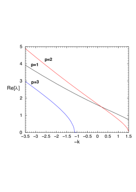
Figure 5: (Color online) The same as in Fig. 4, but for $q=-4$.

The computation of the stability eigenvalues by means of Eq. (36) demonstrates, in the right panels of Figs. 4 and 5, that all the HV modes are subject to instability against small perturbations with various values of azimuthal index $p$. Direct simulations reveal two different scenarios of the instability development, which are displayed in Figs. 6 and 7. In the former case, the central core is spontaneously expelled from the vortex ring, which tends to transform itself into a fundamental mode. In the latter case, the vortex ring splits into two fragments, which is a typical outcome of the instability development of vortices in models with the cubic nonlinearity [25]-[28].

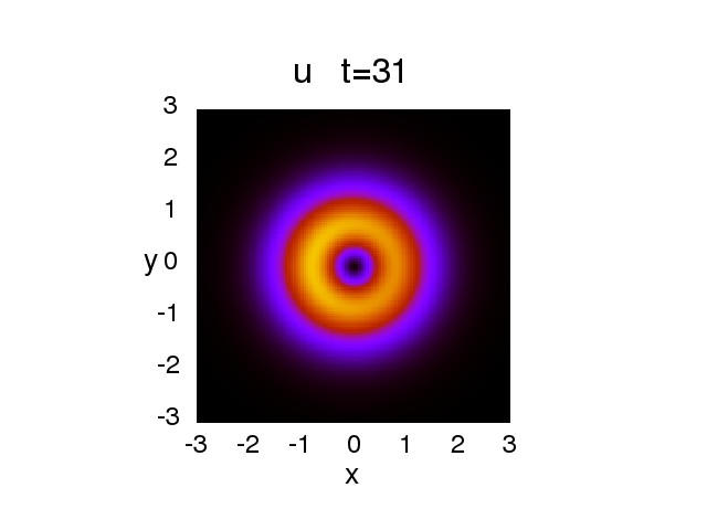
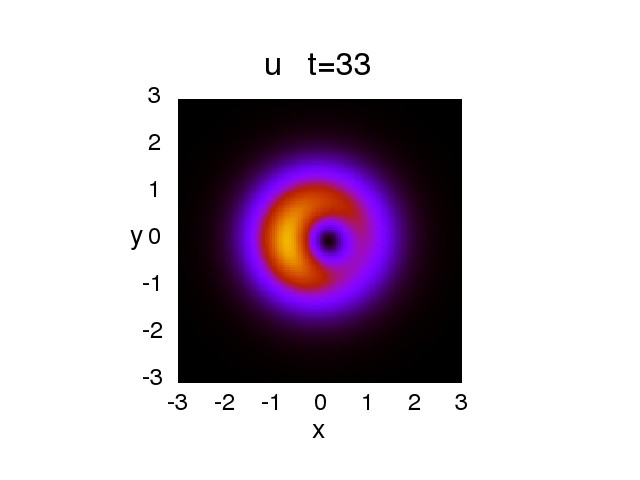
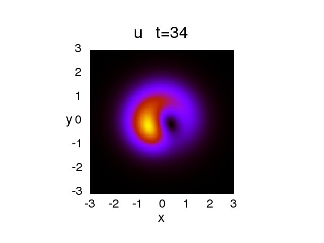
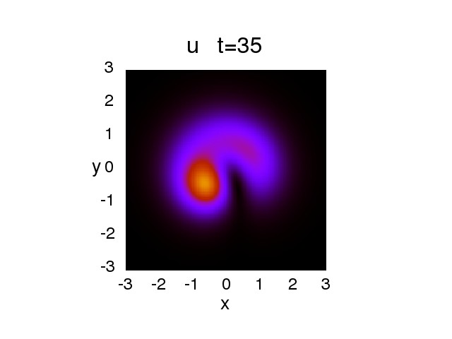
Figure 6: (Color online) The evolution of the two components, $u$, of an unstable hidden-vorticity mode with $q=-4$, norms $N_{u,v}=25.1$, $N_{w}=52.8$ (the total power is $N=103$) and $k=-1$. Density distributions are displayed for values of the propagation distance indicated above the respective panels.

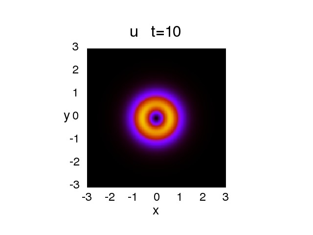
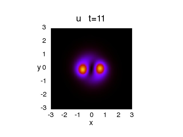
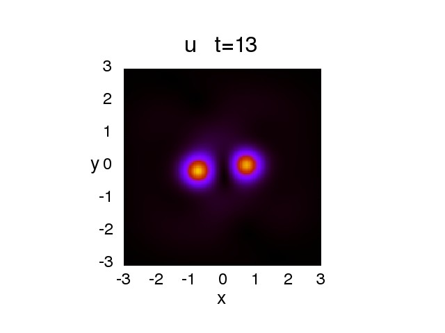
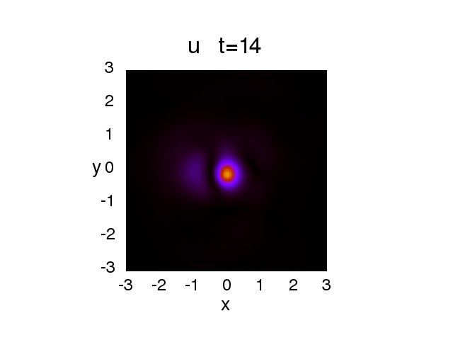
Figure 7: (Color online) The same as in Fig. 6, but for $q=-4$ and $N_{u,v}=340$, $N_{w}=480$, the total power is $N=1160$, and $k=2$.

7.2 Semi-vortices with $S_{u,v,w}=\left(1,0,1\right)$

For families of semi-vortex solutions, a numerical solution of Eq. (22) produces dependences between the propagation constant and integral powers of the three components, a typical example of which is displayed in Fig. 8. It is concluded that these families are completely unstable too.

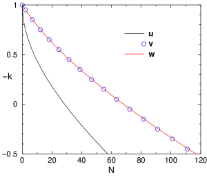
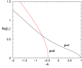
Figure 8: (Color online) Left: Relations between the propagation constant and integral powers of the three fields for semi-vortices of the type of $S_{u,v,w}=\left(1,0,1\right)$, with $\Omega=1$, $Q=0,$ $q=0$. Right: The largest real parts of stability eigenvalues for the semi-vortices, as obtained from the numerical solution of Eq. (36). Integers $p$ are azimuthal indices of the destabilizing perturbation eigenmodes.

Simulations of the instability development of the semi-vortices reveal two basic outcomes which initially look similar to those shown above for the HV modes, cf. Figs. 6 and 7, i.e., expulsion of the central core from the vortex ring, as shown in Fig. 9, or splitting of the vortex into a set of two fragments, see Fig. 10.

Figure 9: (Color online) The evolution of the densities of the $u,v,w$ fields in an unstable semi-vortex corresponding to $k=-0.5$ in Fig. 8.

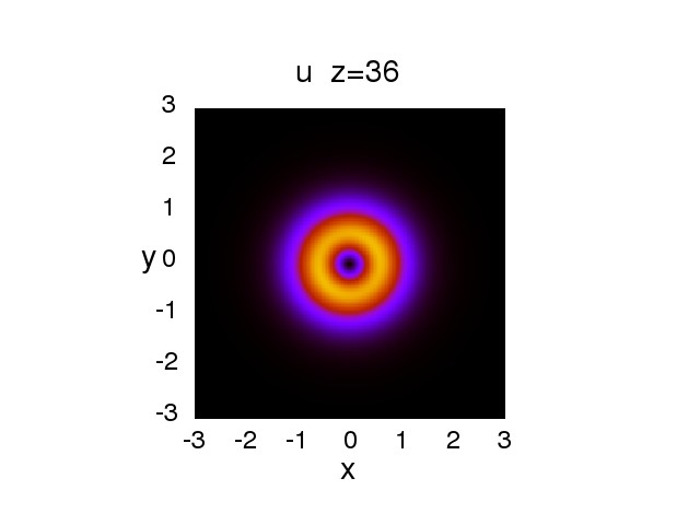
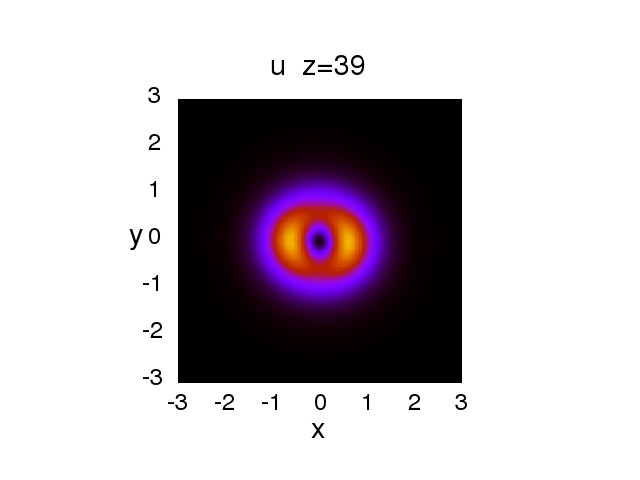
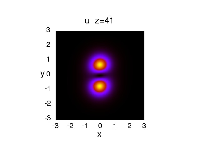
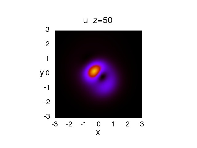
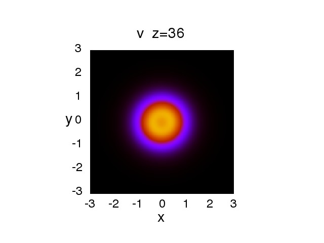
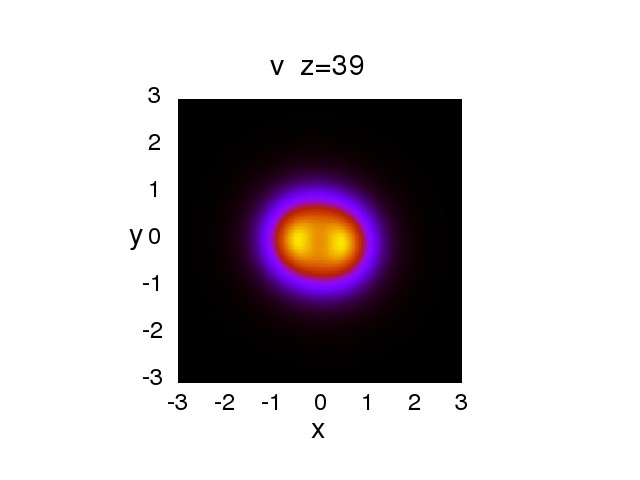
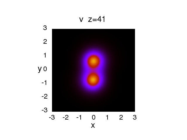
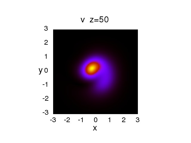
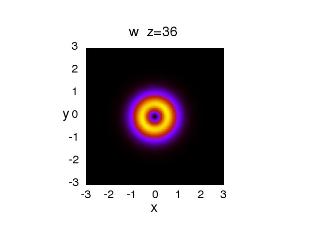
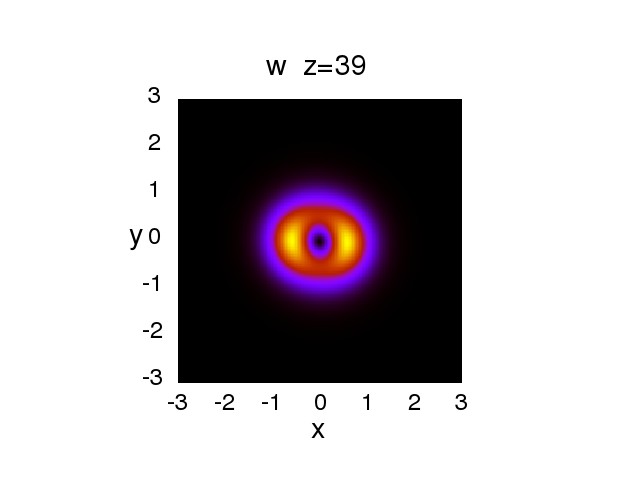
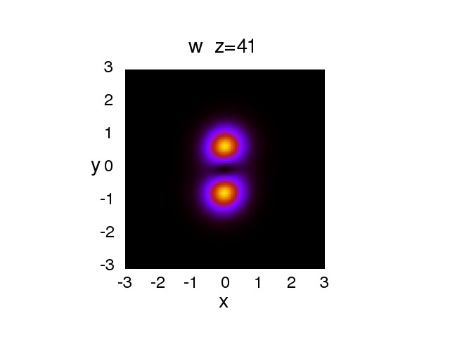
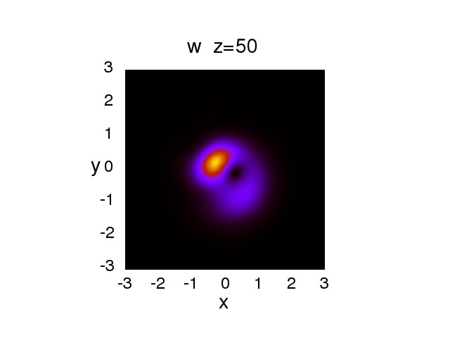
Figure 10: (Color online) The same as in Fig. 9, but for an unstable vortex ring corresponding to $k=1$ .

7.3 Full three-wave vortices

The most general three-wave vortex state is built with $S_{u,v,w}=(1,1,2)$. Families of these solutions were found for the symmetric system, with $Q=0$ and $k_{u}=k_{v}\equiv k$ [see Eqs. (4) and (5)] from a numerical solution of Eq. (25). Their stability eigenvalues were then computed using Eq. (36), and the predicted stability or instability was verified by direct simulations of Eqs. (1)-(3).

A crucial difference of the three-wave vortices from the single-color (SH-only), HV and SV states, which were considered above, is that the full vortices have a well-defined stability area. A typical vortex family and its stability are presented in Fig. 11. This figure explicitly displays both the bifurcation, which generates the full vortex from the corresponding single-color state, with $S_{w}=2$ (as shown above, the bifurcation simultaneously destabilizes the single-color state), and the point of the destabilization of the three-wave vortices.

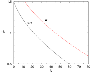
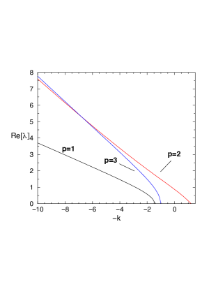
Figure 11: (Color online) Left: The relation between the propagation constant and integral powers of the three components in three-wave vortices with $S_{u,v,w}=(1,1,2)$, $\Omega=1$, $Q=0,q=0$. Solid and dashed lines represent stable and unstable states, respectively. The transition from the single-color state (the emergence of the FF components) occurs at $N_{w}=11.8$. The destabilization takes place at $k=-1.16$, $N_{u,v}=12.5$, $N_{w}=32.0$, the total power being $57.0$. Right: Instability eigenvalues with the largest real part, as found from the numerical solution of linearized equations (36).

The results of the stability analysis are summarized, in the plane of the phase-mismatch parameter, $q$, and total power, $N$, in Fig. 12. The shape of the stability diagram is qualitatively similar to the one which was recently reported, for the degenerate two-wave $\chi^{(2)}$ system, in Ref. [31] (for the sake of the comparison, note that $q$ was defined with the opposite sign in Ref. [31]). The bottom-right area in the diagram is populated by the single-color (SH-only) vortices with $S_{w}=2$, the bifurcation destabilizing the single-color vortex and replacing it by the three-wave one occurring along the upper boundary of this area.

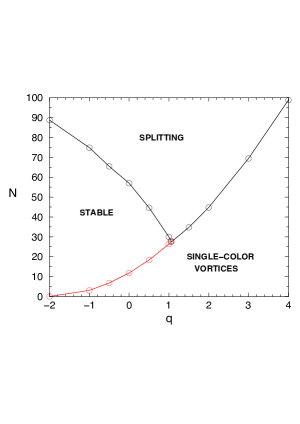
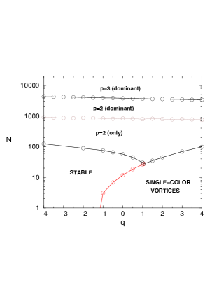
Figure 12: (Color online) Left: The stability diagram for vortices with $S_{u,v,w}=(1,1,2)$, $\Omega=1$, $Q=0$, in the plane of the mismatch parameter ($q$) and total power ($N$). Right: The same, on the logarithmic scale of $N$. In this panel, dominant values of the perturbation azimuthal index are displayed in the region of the splitting instability (label “only” implies that there is a single instability eigenmode in the respective area).

In the “splitting” area labeled in Fig. 12, the three-wave vortices are subject to an instability which splits them into a set of fragments, the number of which is equal to the dominant (or single) azimuthal index, $p$, of unstable perturbation modes, which is indicated in the right panel of the figure. Further, in the region labeled “$p=2$ (only)”, the stable static three-wave vortices are replaced by a robust dynamical regime, in the form of periodic splittings of the vortex into two segments and their recombinations, as shown in Fig. 13. In the course of this periodic evolution, the vortical structure of the mode is conserved. A similar dynamical regime, in the form of periodic splittings and recombinations, is known in the 2D GP equation with the cubic self-attractive nonlinearity and HO trapping potential [27]. On the other hand, the instability-induced splitting the vortex into a set of three fragments is irreversible, as shown in Fig. 14.

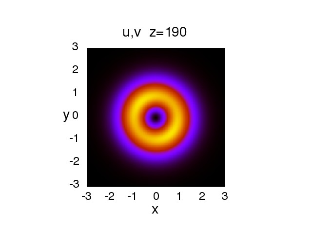
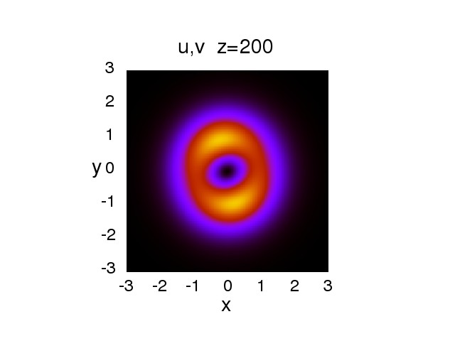
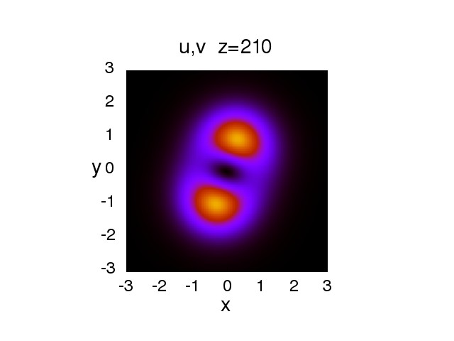
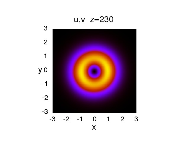
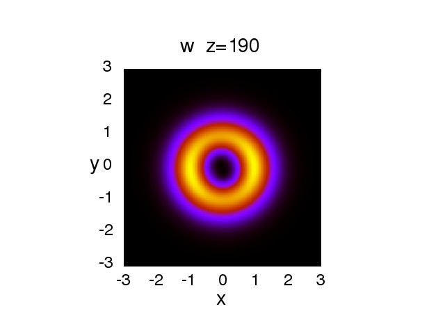
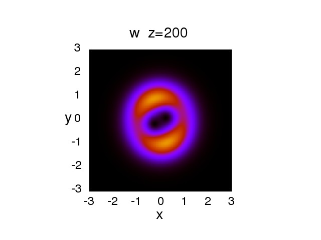
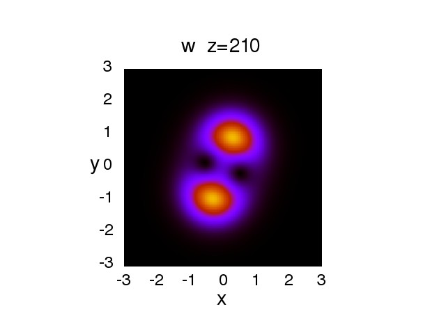
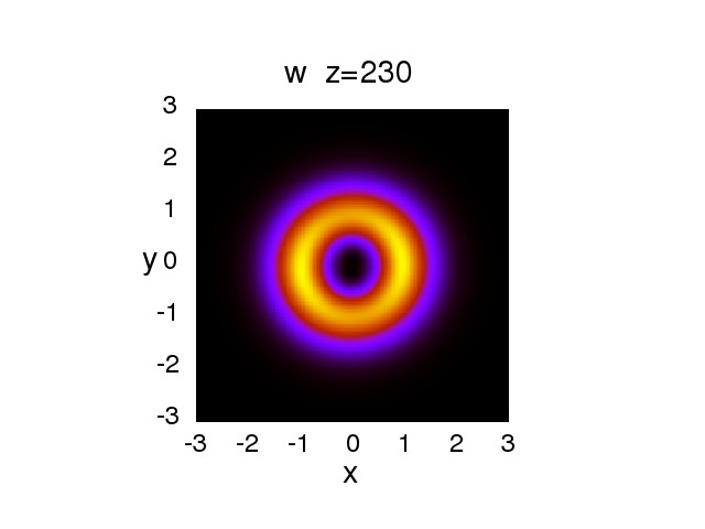
Figure 13: (Color online) The evolution of the densities of the $u,v,w$ fields in the regime of periodic splittings and recombinations of the three-wave vortex, with $S_{u,v,w}=(1,1,2)$, $\Omega=1$, $Q=0,q=0$, $k=-1$, $N_{u,v}=21.4$, $N_{w}=44.4$, the total power being $N=87.2$.

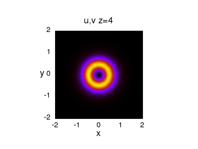
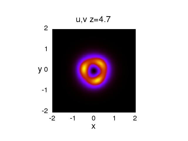
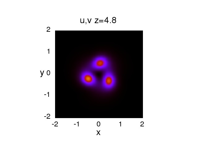
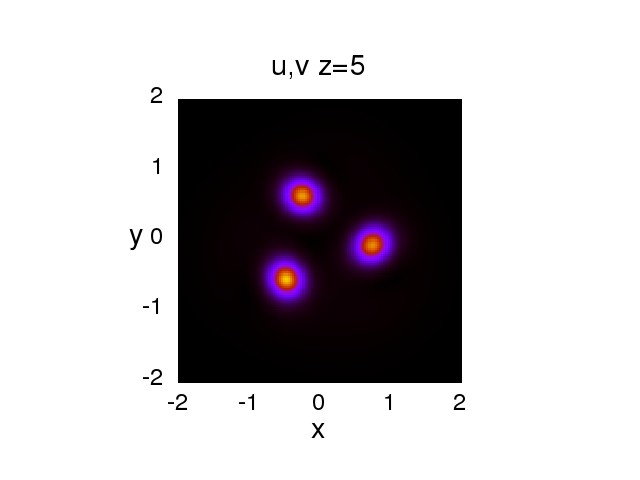
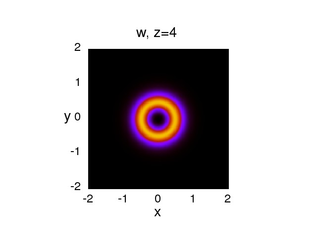
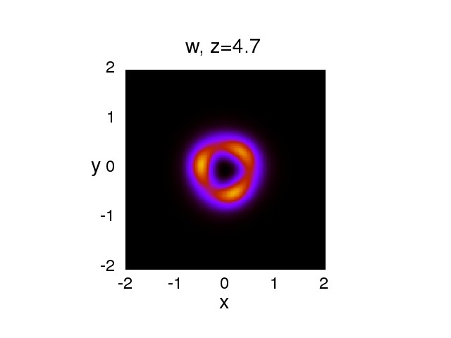
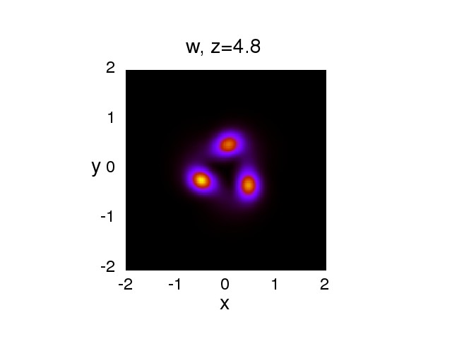
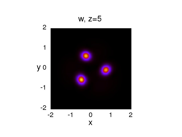
Figure 14: (Color online) An example of the irreversible splitting of the three-wave vortex with $S_{u,v,w}=(1,1,2)$. Top: The evolution of densities of the FF fields, $u$ and $v$, for $\Omega=1$, $Q=0,q=0$, $k=10$, $N_{u,v}=1800$, $N_{w}=2142$, the total power being $N=5741$. Bottom: The same but for the SH  field, $w$.

Finally, the effect of the birefringence of the stability of the three-wave vortices, represented by $Q=1$ in Eqs. (1)-(2), was briefly considered too. As shown in Fig. 15, the birefringence terms make the stability area somewhat larger. This result can be explained by the fact that the birefringence renders the system less coherent, while the splitting instability of the vortices is a result of highly coherent $\chi^{(2)}$ interactions.

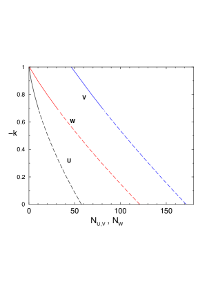
Figure 15: (Color online) The same as in the right panel of Fig. 11, but with $Q=1$ in Eqs. (1)-(2).

8 Conclusion

This work aimed to explore the possibility of the stabilization of various 2D three-wave modes supported by the $\chi^{(2)}$ interactions in the combination with the isotropic HO (harmonic-oscillator) trapping potential. The existence and stability of the modes is determined by powers and vorticities of the three components and the mismatch of the $\chi^{(2)}$ system ($q$). First, using both numerical computations and the VA (variational approximation), stability boundaries were identified for the fundamental (zero-vorticity) and vortical single-color states, in which only the SH (second-harmonic) component is present. On the contrary to the usual assumption that the single-color SH modes are subject to the parametric instability against perturbations in the FF (fundamental-frequency) fields, we have found that they are stable below the respective critical values of the total power. Next, HV (hidden-vorticity) and SV (semi-vortex) states, with vorticities, respectively, $\pm 1$ or $1$ and $0$ in the two FF components, were found to be always unstable. The stability region has been identified for the full three-wave vortices. Furthermore, adjacent to it is the region which features the robust dynamical regime of periodic splitting into two fragments and their recombination into the original vortex.

The analysis reported in the present work can be extended in other directions. One possibility is to analyze asymmetric three-wave modes, with unequal propagation constants in the two components of the FF field. It may also be interesting to construct self-trapped three-wave $\chi^{(2)}$ modes supported by a periodic (lattice) potential, instead of the HO, cf. Ref. [45]. Lastly, a challenging possibility is to construct three-dimensional three-wave “light bullets” supported by the HO trapping potential, cf. Ref. [32] where this was done for the degenerate two-wave system.

A.G. would like to thank the Brazilian funding agencies Fundação de Amparo à Pesquisa do Estado de São Paulo and Conselho Nacional de Desenvolvimento Científico e Tecnológico. B.A.M. acknowledges a visitor’s grant provided by South American Institute for Fundamental Research (Sao Paulo).

References

• [1] Stegeman G I, Hagan D J and Torner L 1996 Opt. Quant. Electr. 28 1691-1740
• [2] Etrich C, Lederer F, Malomed B A, Peschel T and Peschel U 2000 Progr. Opt. 41 483-568
• [3] Buryak A V, Di Trapani P, Skryabin D V and S. Trillo S. 2002 Phys. Rep. 370 63-235
• [4] Malomed B A, Mihalache D, Wise F and Torner L 2005 J. Optics B: Quant. Semicl. Opt. 7, R53-R72
• [5] Kivshar Y S and Agrawal G P 2003, Optical Solitons: From Fibers to Photonic Crystals (San Diego, CA: Academic)
• [6] Du F, Lu Y W and Wu S T 2004 Appl. Phys. Lett. 85 2181-2183
• [7] Luan F, George A K, Hedeley T D, Pearce G J, Bird D M, Knight J C and Russell P S J 2004 Opt. Lett. 29 2369-2371
• [8] Kanashov A A and Rubenchik A M 1981 Physica D 4, 122-134
• [9] Torruellas W E, Wang Z, Hagan D J, VanStryland E W, Stegeman G I, Torner L and Menyuk C R 1995 Phys. Rev. Lett. 74 5036-5039
• [10] Malomed B A, Drummond P, He H, Berntson A, Anderson D and Lisak M 1997 Phys. Rev. E 56 4725-4735
• [11] Liu X, Qian L J and Wise F W 1999 Phys. Rev. Lett. 82 4631-4634
• [12] Liu X, Beckwitt K and Wise F 2000 Phys. Rev. E 62 1328-1340
• [13] Bovino F A, Braccini M and Sibilia C 2011 J. Opt. Soc. Am. B 28 2806-2811
• [14] Firth W J and Skryabin D V 1997 Phys. Rev. Lett. 79 2450-2453
• [15] Torner L and Petrov D V 1997 Electron. Lett. 33 608-610
• [16] Skryabin D V and Firth W J 1998 Phys. Rev. E 58 R1252-R1255
• [17] Torres J P, Soto-Crespo J M, Torner L and Petrov D V 1998 J. Opt. Soc. Am. B 15 625-627
• [18] Petrov D V, Torner L, Martorell J, Vilaseca R, Torres J P and Cojocaru C 1998 Opt. Lett. 23 1444-1446
• [19] Torres J P, Soto-Crespo J M, Torner L and Petrov D V 1998 Opt. Commun. 149 77-83
• [20] Molina-Terriza G, Wright E M and Torner L 2001 Opt. Lett. 26 163-165
• [21] Kruglov V I, Logvin Y A and Volkov V M 1992 J. Mod. Opt. 39 2277-2291
• [22] Pethick C J and Smith H 2008 Bose-Einstein condensate in dilute gas (Cambridge University Press: Cambridge)
• [23] Dalfovo F and Stringari S 1996 Phys. Rev. A 53 2477-2485
• [24] Dodd R J 1996 J. Res. Natl. Inst. Stand. Technol. 101 545-552
• [25] Alexander T J and BergΓ© L 2002 Phys. Rev. E 65 026611
• [26] Carr L D and Clark C W 2006 Phys. Rev. Lett. 97 010403
• [27] Mihalache D, Mazilu D, Malomed B A and Lederer F 2006 Phys. Rev. A 73 043615
• [28] Carr L D and Clark C W 2006 Phys. Rev. A 74 043613
• [29] Herring G, Carr L D, Carretero-GonzΓ‘lez R, Kevrekidis P G and Frantzeskakis D J 2008 Phys. Rev. A 77 043607
• [30] Sakaguchi H, Li B and Malomed B A 2014 Phys. Rev. E 89 032920
• [31] Sakaguchi H and Malomed B A 2012, J. Opt. Soc. Am. B 29 2741
• [32] Sakaguchi H and B. A. Malomed 2013 Opt. Exp. 21 9813-9823
• [33] Drummond P D, Kheruntsyan K V and He H 1998 Phys. Rev. Lett. 81 3055-3058
• [34] Heinzen D J, Wynar R, Drummond P D and Kheruntsyan K V 2000 Phys. Rev. Lett. 84 5029-5033
• [35] Hope J J and Olsen M K 2001 Phys. Rev. Lett. 86 3220-3223
• [36] Hornung T, Gordienko S, de Vivie-Riedle R and Verhaar 2002 Phys. Rev. A 66 043607
• [37] Torres J P, Soto-Crespo J M, Torner L and Petrov D V 1998 Opt. Commun. 149 77-83
• [38] Desyatnikov A S, Mihalache D, Mazilu D, Malomed B A, Denz C and Lederer F 2005 Phys. Rev. E 71 026615
• [39] Leblond H, Malomed B A and Mihalache D 2005 Phys. Rev. E 71 036608
• [40] Desyatnikov A S, Mihalache D, Mazilu D, Malomed B A and Lederer F 2007 Phys. Lett. A 364 231-234
• [41] Brtka M, Gammal A and Malomed B A 2010 Phys. Rev. A 82 053610
• [42] Kevrekidis P G and Pelinovsky D E 2006 Proc. R. Soc. A 462 2671-2694
• [43] Leykam D, Malomed B and Desyatnikov A S 2013 J. Optics 15 044016
• [44] Ye F, Wang J, Dong L, and Li Y 2004, Opt. Commun. 230 219-223
• [45] Xu Z Y, Kartashov Y V, Crasovan L C, Mihalache D and Torner L 2005 Phys. Rev. E 71 016616