Deterministic Diffusion

Abstract

In the present paper, we give a series of definitions and properties of Lifting Dynamical Systems (LDS) corresponding to the notion of deterministic diffusion. We present heuristic explanations of the mechanism of formation of deterministic diffusion in LDS and the anomalous deterministic diffusion in the case of transportation in long billiard channels with spatially periodic structures. The expressions for the coefficient of deterministic diffusion are obtained.

Key words: dynamical system, one-dimensional lifting dynamical system, deterministic diffusion, anomalous diffusion, diffusion coefficient, billiard channel, nonideal reflection law.

1 Introduction

One-dimensional dynamical systems on the entire axis with discrete time are defined by the recurrence relation

$$x_{n+1}=f(x_{n}),$$ (1)

where $f(x)$ is a real function given on the entire axis and $x_{0}$ is a given initial value [8, 14]. Equation (1) determines a trajectory $(x_{0},x_{1},...,x_{n},...)=x$ in the dynamical system (1) according to the initial value $x_{0}$ and the form of the function $f.$ For the dynamical systems admitting the chaotic behavior of trajectories, the problem of construction of the entire trajectory or even of determination of the values of $x_{n}$ for large $n$ is quite complicated because, as a rule, the numerical calculations are performed with a certain accuracy and the dependence of the subsequent values of $x_{n}$ on the variations of the previous values is unstable. Moreover, from the physical point of view, the initial value $x_{0}$ is specified with a certain accuracy. Therefore for the investigation of the behavior of trajectories for large values of time, we can analyze not the evolution of system (1) but the evolution of measures on the axis generated by this evolution.

If a probability measure $\mu_{0}$ (a normalized measure for which the measure of the entire axis is equal to 1) with density $\rho_{0}:$ $\mu_{0}(A)=\int\limits_{A}\,\rho_{0}(x)\,dx$ is given at the initial time, then, for a unit of time, system (1) maps this measure into $\mu_{1}:$ $\mu_{1}(A)=\mu(f^{-1}(A)),$ where $f^{-1}(A)$ is a complete preimage of the set $A$ under the map $f.$ The operator mapping the measure $\mu_{0}$ into the measure $\mu_{1}$ is called a Perron–Frobenius operator. The Perron–Frobenius operator $\mathcal{F}$ is linear even for nonlinear dynamical systems (1) and maps the density $\rho_{0}$ of the initial measure into the density $\rho_{1}$ of the measure $\mu_{1}$ as the integral operator with singular kernel containing a Dirac $\delta$ function:

$$\rho_{1}(x)=\mathcal{F}\rho_{0}(x)=\int\,\delta(x-f(y))\rho_{0}(y)\,dy=\sum_{y_{k}\in f^{-1}(\{x\})}\,\frac{1}{|f^{\prime}(y_{k})|}\rho_{0}(y_{k}).$$ (2)

The investigation of the asymptotic behavior of the density $\rho_{n}=\mathcal{F}^{n}\rho_{0}$ as $n\rightarrow\infty$ is reduced to the investigation of the behavior of the semigroup $\mathcal{F}^{n}.$ There are examples of dynamical systems (1) with locally stretching maps $f$ for which the densities $\rho_{n}$ are asymptotically Gaussian as $n\rightarrow\infty$ independently of the choice of the density of the initial probability measure. In this case, it is said that deterministic diffusion occurs in the dynamical system (1).

The aim of the present paper is to consider examples of dynamical systems with deterministic diffusion. We restrict ourselves to the so-called lifting dynamical systems (LDS) with piecewise linear functions $f(x)$ in DS (1).

We briefly consider the mechanisms of appearance of the anomalous deterministic diffusion in the process of transportation in long billiard channels with spatially periodic structures.

2 Lifting Dynamical System

Consider the dynamical system (1) on the entire axis, where the function $f(x)$ is given on the main interval $I_{0}=[-\frac{1}{2},\frac{1}{2}).$ The function $s(x)=f(x)-x$ with $x\in I_{0}$ has the sense of a shift of the point $x$ under the map $f.$ We split the entire axis $(-\infty,\infty)$ into disjoint intervals $I_{k}=[k-\frac{1}{2},k+\frac{1}{2}),$ where $k\in Z$ are integers. Assume that the function $f$ is extended from the interval $I_{0}$ onto all intervals $I_{k}$ so that the shift of a point under the map $f$ on each interval $k$ is the same as on $I_{0},$ that is $s(k+x)=f(k+x)-(k+x)=s(x)=f(x)-x.$ This gives a periodic shift function $s(x)$ and implies the periodicity of the function $f$ with lift 1

$$f(k+x)=k+f(x),\,|x|<\frac{1}{2},\,\,k\in Z.$$ (3)

The dynamical system (1) with a function $f$ satisfying property (3) is called a LDS. This dynamical system (DS) is well known and thoroughly investigated [4, 8, 9].

Lemma.

Let a function $f$ defined on the interval $I_{0}=[-\frac{1}{2},\frac{1}{2})$ be a piecewise monotone stretching function on a finite partition $\{I_{0,j}\}_{j=1}^{m}$ of the interval $I_{0}=\bigcup\limits_{j=1}^{m}I_{0,j},$ i.e., there exists $\lambda>1$ such that

$$|f(x)-f(y)|\geq\lambda|x-y|$$ (4)

for $x,y\in I_{0,k},$ and, in addition, the function $f(x)$ has finite nonzero discontinuities at the points of joint of the intervals $I_{0,j}.$ Then the periodic extension (3) with lift 1 specifies a locally stretching function $f$ on the entire axis.

Proof.

If the points $x$ and $y$ belong to the same interval $I_{0,k},$ then, by virtue of (4),

$$|f(x)-f(y)|=|f(x-k)-f(y-k)|\geq\lambda|x-y|.$$

If the points $x$ and $y$ belong to neighboring intervals, then the function has a discontinuity at the point of joint of these intervals and the value of this discontinuity is not smaller than a certain $a>0.$ In view of the monotonicity of the function $f,$ there exists $\varepsilon_{0}>0$ such that, for $|x-y|<\varepsilon_{0},$ the points $x$ and $y$ belong either to the same interval $I_{0,k}$ or to neighboring intervals. Hence,

$$|f(x)-f(y)|\geq\frac{a}{3}\geq\lambda\varepsilon,$$

where $\varepsilon=\min(\varepsilon_{0},\frac{a}{3\lambda}).$ Thus, for $|x-y|<\varepsilon,$ we have $|f(x)-f(y)|\geq\lambda|x-y|.$ ∎

Let $x=(x_{0},x_{1},...,x_{n},...)$ be a trajectory for the LDS (1)–(3). By $k,$ we denote the number of the interval $I_{k}=[k-\frac{1}{2},k+\frac{1}{2})$ containing a number $a\in I_{k}$ as follows: $k=[a)$ is the nearest integer for the number $a.$ Then the trajectory $x$ is associated with an integer-valued sequence: $M=([x_{0}),[x_{1}),...,[x_{n}),...)=(m_{1},m_{2},...,m_{n},...)$ of the numbers of intervals containing the values $x_{n}.$ The sequence $M$ is called the route of the trajectory $x$ and contains the numbers of intervals successively “visited” by the phase point in the LDS [8].

Proposition 1.

Let the function $f$ determining the LDS (1)–(3) be stretching. Then the trajectory of the LDS is uniquely determined by its route.

Proof.

Assume that two initial conditions $x_{0}^{(1)}$ and $x_{0}^{(2)}$ generate trajectories of the LDS with the same route. This means that the points $x_{n}^{(1)}$ and $x_{n}^{(2)}$ lie in the same interval $I_{m_{n}}.$ In view of the stretching property of the map $f,$ the inequality $|x_{n+1}^{(1)}-x_{n+}^{(2)}|\geq\lambda|x_{n}^{(1)}-x_{n}^{(2)}|,$  $\lambda>1,$ is true. Since any two points from the same interval $I_{m_{n}}$ differ by at most 1, the successive application of this inequality yields the inequality $|x_{0}^{(1)}-x_{0}^{(2)}|\leq\frac{1}{\lambda^{n}}$ for any $n.$ Since $\lambda>1,$ this implies that $x_{0}^{(1)}=x_{0}^{(2)}.$ ∎

Definition 1.

If any integer-valued sequence in the LDS is a route of a certain trajectory and the trajectory is uniquely determined by its route, then we say that the LDS possesses the Bernoulli property [8].

Proposition 2.

If a function $f$ defined in the interval $I_{0}=[-\frac{1}{2},\frac{1}{2})$ is odd, continuous, monotonically increasing, stretching, and unbounded, then the LDS (1)–(3) corresponding to this function $f$ possesses the Bernoulli property.

Proof.

The uniqueness of reconstruction of a trajectory according to its route is proved in Appendix 1. Let $M=(m_{1},m_{2},...,m_{n},...)$ be an arbitrary integer-valued sequence. In the interval $I_{m_{1}},$ we consider a sequence of embedded contracting closed intervals $U_{n}$ constructed as follows:

Let $U^{(1)}$ be the closure of the preimage of the interval $I_{m_{n}}$ under the map $f$ lying on $I_{m_{n-1}}$ : $U^{(1)}=f^{-1}(I_{m_{n}}).$ Since the map $f$ is stretching, the length $\mathrm{mes}\,U^{(1)}\leq\lambda^{-1}.$ Let $U^{(2)}$ be the preimage of $U^{(1)}$ in the interval $I_{m_{n-2}}$ and let, by induction, $U^{(k)}$ be the preimage of $U^{(k-1)}$ in the interval $I_{m_{n-k}}.$ The sets $U_{n}=U^{(n)}\subset I_{m_{1}}$ and $\mathrm{mes}\,U_{n}\leq\lambda^{n}.$ As $n\rightarrow\infty,$ we get a system of embedded closed sets $U_{n+1}\subset U_{n}$ in the interval $I_{m_{k}}$ and $\mathrm{mes}\,U_{n}\rightarrow 0$ as $n\rightarrow\infty.$ The common limit point $x_{0}$ for all $U_{n}$ lies in $I_{m_{1}}$ and its trajectory $x=(x_{0},f(x_{0}),...,f^{n}(x_{0}),...)$ has the route $M.$ ∎

3 Markov Partition of the Phase Space of LDS. Piecewise Linear LDS

The system of intervals $I_{k}=[k-\frac{1}{2},k+\frac{1}{2}),$ $k\in Z,$ for the LDS (1)–(3) can be regarded as a Markov partition of the phase space [8]. Consider a finer Markov subpartition. Assume that the main interval $I_{0}$ is split into finitely many $m$ subintervals $I_{0,j}=[x_{j},x_{j+1}),$ where $x_{0}=-\frac{1}{2},$ $x_{j}<x_{j+1},$ $x_{m}=\frac{1}{2},$ $j=0,1,2,...,m,$ and $I_{0,j}=[x_{j-1},x_{j}).$ An integer-valued shift of this partition leads to the decomposition of the intervals $I_{k}$ into subintervals $I_{k,j}=[k+x_{j-1},k+x_{j}).$ Hence, the entire axis is split into intervals $\{I_{k,j}\},$  $k\in Z,$   $j=1,2,...,m.$

Definition 2.

We say that the Markov partition $\{I_{k,j}\}_{k\in Z,1\leq j\leq m}$ of the entire axis is consistent with the LDS (1)–(3) if the LDS maps, for a unit of time, any probability measure with constant densities in each set $I_{k,j}$ into a measure with constant densities in each interval $I_{k,j}$.

Definition 3.

We say that a function $f$ specifying the LDS (1)–(3) is consistent with the Markov partition $\{I_{k,j}\}_{k\in Z,1\leq j\leq m}$ defined with the help of the numbers $-\frac{1}{2}=x_{0},x_{1},...,x_{m}=\frac{1}{2}$ if it is linear and nonconstant on each interval $I_{k,j}$ and, at each end of the interval $I_{k,j},$ takes values equal to an integer plus one of the numbers $x_{j},$  $j=0,1,...,m.$

Example 1.

Let $f(x)=\Lambda x$ be a linear function in the interval $I_{0}=[-\frac{1}{2},\frac{1}{2}),$ where $\Lambda=2l+1$ is an odd number. Then this function is consistent with the Markov partition $\{I_{k}\}_{k\in Z},$ $I_{k}=[k-\frac{1}{2},k+\frac{1}{2}).$

Example 2.

Let $f(x)=\Lambda x,$ where $\Lambda=2l$ is an even number. Then this function is consistent with the Markov partition $\{I_{k,\pm}\}_{k\in Z},$ where $I_{k,+}=[k,k+\frac{1}{2})$ and $I_{k,-}=[k-\frac{1}{2},k).$

An important example of the function $f$ satisfying Definition 3 is given by the following assertion:

Proposition 3.

Assume that a function $f(x)$ determining the LDS in the interval $I_{0}$ is piecewise linear, takes half-integer values at the ends of each its linear pieces, and moreover, $f^{\prime}(x)\neq 0$ almost everywhere. Then, by Definition 3, the function $f$ is consistent with the Markov partition $\{I_{k}\}|_{k\in Z}.$

Proof.

The proof follows from the verification of the conditions of Definition 3 for points $\{x_{j}\},$ that is for all points at which the function $f$ takes half-integer values. ∎

A piecewise linear function $f$ from Proposition 3 will be called a piecewise linear function taking half-integer values at the ends of the linear pieces.

The equivalence of Definitions 2 and 3 for LDS yields the following statement:

Proposition 4.

For the Markov partition $\{I_{n,j}\}_{n\in Z,|j|\leq m}$ to be consistent with the action of the LDS (1)–(3) by Definition 2, it is necessary and sufficient that the function $f$ determining the LDS (1)–(3) be consistent with this Markov partition by Definition 3.

Proof.

We now show that if $f$ satisfies the conditions of Definition 3, then the LDS transforms the probability measure with constant densities on $I_{n,j}$ into a measure with constant densities on $I_{n,k},$ i.e., the LDS satisfies the conditions of Definition 2. Since operator (2) is linear, it suffices to consider the case where the density of the initial measure is constant on the fixed interval $I_{n_{0},k_{0}}.$ On this interval, the function $f(x)$ is linear and nonconstant and maps $I_{n_{0},k_{0}}$ into the union $\bigcup I_{n,k}$ of several neighboring intervals. Therefore, the inverse map of these intervals is linear and, hence, the measure has a constant density in each of these intervals.

Let the conditions of Definition 2 be satisfied. If the density of the initial measure is constant in the interval $I_{n_{0},k_{0}},$ then the map $f$ gives a new measure $\mu_{1}$ on the entire axis. It is clear that $\mathrm{supp}\,\mu$ coincides with the closure of a certain union $f^{-1}(I_{n,k})=\bigcup I_{0,j}$ because, otherwise, there exist an interval $I_{\bar{n},\bar{k}}$ and its part $A$ such that $\mu_{1}(I_{\bar{n},\bar{k}})=\mu_{1}(A)\neq 0$ and $\mu_{1}(A)=0.$ This contradicts the condition of Definition 2 according to which the measure $\mu_{1}$ has a constant density. Let $I_{\bar{n},\bar{k}}$ be one of the intervals $f(I_{n_{0},k_{0}})$ and let $B=f^{-1}(I_{\bar{n},\bar{k}}).$ Since $B\subset I_{n_{0},k_{0}},$ the initial measure on $B$ has a constant density, $f$ bijectively maps $B$ onto $I_{\bar{n},\bar{k}},$ and, according to the Perron–Frobenius operator, the density $\rho_{1}(x)$ of the measure $\mu_{1}$ on $I_{\bar{n},\bar{k}}$ is expressed via the density $\rho_{0}$ of the initial measure on $I_{n_{0},k_{0}}$ by the equality $\rho_{1}(x)=\frac{\rho_{0}(x)}{|f^{\prime}(x)|}.$ Thus, we arrive at the conclusion that $f^{\prime}(x)\equiv const$ on the interval $B$ and that the function maps the ends of the interval $B$ into the ends of the interval $I_{\bar{n},\bar{k}}.$ Thus, the function $f$ satisfies the conditions of Definition 3. ∎

The following question arises: Is it possible to construct Markov partitions of the entire axis consistent with the linear function $f(x)=\Lambda x$ for the values of $\Lambda$ other than in Examples 1 and 2?

Since the linear function $f(x)=\Lambda x$ is odd, the numbers $x_{j}$ specifying a consistent Markov subpartition of the interval $I_{0}$ are symmetric about the middle of the interval $I_{0}.$ Hence, it is sufficient to define solely the positive values of $x_{j}$ and indicate that the number $m$ of subintervals $\{I_{0,j}\}_{1\leq j\leq m}$ is even or odd, because $s=0$ belongs to the set $\{s_{j}\}$ for even $m$ and does not belong to this set for odd $m.$

We enumerate the ends of the intervals $\{I_{k,j}\}$ located on the positive half axis in the order of increase starting from the first positive number. This yields a sequence $0<s_{0}<s_{1}<s_{2}<...<s_{k}<....$ Since the Markov subpartition $\{I_{k,j}\}$ is consistent with the LDS with the linear function $f(x)=\Lambda x,$ we get

$$\Lambda s_{1}=s_{1+n_{1}},\,\Lambda s_{2}=\Lambda s_{1+n_{1}+n_{2}},...,\Lambda s_{\hat{m}}=s_{1+n_{1}+n_{2}+...+n_{\hat{m}}}.$$ (5)

Here, $\hat{m}$ is expressed via $m$ of the form $m=2\hat{m}$ for even $m$ and of the form $m=2\hat{m}-1$ for odd $m.$ Hence, each Markov subpartition of the axis consistent with the linear function $f(x)=\Lambda x$ specifying the LDS (1)–(3) is associated with two parameters: the parity of the number $m$ of subintervals $\{I_{0,j}\}$ (i.e., $s=(-1)^{m}$) and the integer-valued vector $\vec{n}=(n_{1},n_{2},...,n_{\hat{m}}).$ These quantities $(s,\vec{n})$ are called the parameters of the Markov subpartition $\{I_{k,j}\}.$

Proposition 5.

The parameters of the Markov subpartition $\{I_{k,j}\}$, i.e., the parity of the number $m$ and the integer-valued vector $\vec{n}=(n_{1},n_{2},...,n_{\hat{m}})$ uniquely define the quantity $\Lambda,$ the slope of the linear function $f(x)=\Lambda x,$ consistent with the Markov subpartition $\{I_{k,j}\}$ and a collection of numbers $\{s_{j}\}_{j=1}^{\hat{m}}$ specifying the ends of the intervals $I_{k,j}=[k+s_{j},k+s_{j+1})$ of this subpartition.

Proof.

Let the number of components of the vector $\vec{n}$ be equal to $\hat{m}.$ Then the number $m$ of subintervals $\{I_{0,j}\}$ in the Markov subpartition is given by the equality $m=2\hat{m}$ for even $m$ and the equality $m=2\hat{m}-1$ for odd $m$ (the parity of $m$ is specified by the quantity $s=(-1)^{m}$). We always have $s_{\hat{m}}=\frac{1}{2}.$ For odd $m,$ the sequence $s_{1},s_{2},...,s_{k},...$ has the form $s_{1},s_{2},...,s_{\hat{m}+1},\frac{1}{2},1-s_{\hat{m}-1},1-s_{\hat{m}-2},...,1-s_{1},1+s_{1},1+s_{2},...,1+s_{\hat{m}-1},\frac{3}{2},2-s_{\hat{m}-1},...$ and is explicitly expressed via $s_{1},s_{2},...,s_{\hat{m}}=\frac{1}{2}.$ Hence, we can explicitly express each term of the sequence $s_{1},s_{2},...,s_{k},...$ in terms of an integer and one of the numbers $s_{1},s_{2},...,s_{\hat{m}}.$ Thus, equalities (5) turn into a linear system for $s_{1},s_{2},...,s_{\hat{m}}$ whose coefficients are either integers or the quantity $\Lambda.$ The consistency condition for this system can be formulated as the equality of the determinant of this system to zero. This gives the following algebraic equation for $\Lambda$:

$$R_{\vec{n}}(\Lambda)=0.$$

If we find $\Lambda,$ then all $s_{1},s_{2},...,s_{\hat{m}}$ can be uniquely determined from (5). Similarly, we consider the case of even $m.$ In this case, the sequence $s_{1},s_{2},...,s_{k},...$ contains integer values and has the form $s_{1},s_{2},...,s_{\hat{m}}=\frac{1}{2},1-s_{\hat{m}-1},1-s_{\hat{m}-2},...,1-s_{1},0,1+s_{1},1+s_{2},....$ ∎

An implementation of this scheme by a constructive example is given in the next Proposition.

Proposition 6.

A linear function $f(x)=\Lambda x$ determining the LDS (1)–(3) will be consistent with the Markov partition $\{[k-\frac{1}{2},\xi),[k-\xi,k+\xi),[k+\xi,k+\frac{1}{2})\}_{k\in\mathbb{Z}}$, if for integers $0<m<n$ and the values $\varepsilon_{1}=\pm 1$, $\varepsilon_{2}=\pm 1$ we have

$$\Lambda=\frac{2n+\varepsilon_{2}+\sqrt{(2n-\varepsilon_{2})^{2}+8m\varepsilon_{1}}}{2},$$

$$\xi=\frac{2m}{2n-\varepsilon_{2}+\sqrt{(2n-\varepsilon_{2})^{2}+8m\varepsilon_{1}}}.$$

Proof.

This is a consequence of the equalities (5), in this case having the form

$$\Lambda\xi=m+\varepsilon_{2}\xi,$$

$$\frac{\Lambda}{2}=n+\varepsilon_{1}\xi.$$

∎

It is worth noting that the set of values of the slope $\Lambda$ of the linear function $f(x)=\Lambda x,$ $x\in I_{0}=[-\frac{1}{2},\frac{1}{2}),$ for which it is possible to construct Markov partitions consistent with the LDS (1)–(3) is everywhere dense on the half axis $(2,\infty)$ [4, 9].

4 Deterministic Diffusion

We consider the LDS (1)–(3) for which the collection of intervals $\{I_{k}\}_{k\in Z},$  $I_{k}=[k-\frac{1}{2},k+\frac{1}{2}),$ forms a Markov partition of the phase space consistent with the action of the LDS. This means that, for a time unit, the LDS maps the measure $\mu_{0}$ with unit density in the interval $I_{0}$ into a probability measure with constant densities $p_{k}\geq 0$ in the intervals $I_{k}$ and $\sum\limits_{k\in Z}\,p_{k}=1.$ As a result of multiple application of the LDS, the initial measure $\mu_{0}$ is transformed into a measure with constant densities in the intervals $I_{k}.$ Let $P_{k}(n)$ be the density of the measure in the interval $I_{k}$ after the $n$-fold action of the LDS upon the initial measure $\mu_{0}.$ Then

$$P_{k}(n+1)=\sum\limits_{l\in Z}\,p_{k-l}P_{l}(n)$$ (6)

and $P_{k}(0)=\delta_{k,0}$ due to the choice of the initial measure $\mu_{0}.$ The asymptotic behavior of the quantities $P_{k}(n)$ for large $n,$ as solutions of Eq. (6), is described by the well-known central limit theorem of the probability theory [5, 6]. Indeed, if we consider the sum $\xi=\xi_{1}+\xi_{2}+...+\xi_{n}$ of $n$ independent random variables each of which takes only integer values $k$ with probability $p_{k},$ then we get Eq. (6), where $P_{k}(n)$ is the probability of the event that $\xi$ takes the value $k.$

Theorem 1.

Let the numbers $\{p_{k}\}_{k\in Z}$ take nonnegative values such that $\sum\limits_{k\in Z}\,p_{k}=1,$ let the greatest common divisor of the numbers $k$ with $p_{k}>0$ be equal to 1, and let there exist the first and second moments

$$\sigma_{1}=\sum\limits_{k\in Z}\,kp_{k},\quad\sigma^{2}=\sum\limits_{k\in Z}\,k^{2}p_{k}.$$ (7)

Then the solution of Eq. (6) as $n\rightarrow\infty$ has an asymptotics

$$P_{k}(n)-\frac{1}{\sigma\sqrt{2\pi n}}e^{-\frac{(x-\xi_{n})^{2}}{2\sigma^{2}n}}\rightarrow 0$$ (8)

uniformly in $k.$ The character of convergence in (8) depends on additional conditions, e.g., on the existence of the third moment (the Laplace theorem).

Proof.

We now briefly present the well-known scheme of the proof of Theorem 1 based on the fact that Eq. (6) is a difference analog of the convolution equation. As a result of the Fourier transformation, the convolution turns into the product. Let $P(\lambda,n)=\sum\limits_{k\in Z}\,P_{k}(n)e^{ik\lambda}$ be the characteristic function of the solution of Eq. (6), $P(\lambda)=\sum\limits_{k\in Z}\,p_{k}e^{ik\lambda}.$ Thus, we get the following formula from Eq. (6):

$$P(\lambda,n)=[P(\lambda)]^{n}P(\lambda,0).$$ (9)

Since the initial measure is concentrated on $I_{0}$ and its density is constant, we conclude that $P(\lambda,0)=1$ and

$$P_{k}(n)=\frac{1}{2\pi}\int\limits_{-\pi}^{\pi}[P(\lambda)]^{n}e^{-ik\lambda}\,d\lambda$$ (10)

As $\lambda\rightarrow 0,$ $P(\lambda)=\sum\limits_{k\in Z}\,p_{k}e^{ik\lambda}=1+i\sigma_{1}\lambda-\frac{\sigma^{2}\lambda^{2}}{2}+o(1)=e^{i\sigma_{1}\lambda-\frac{\sigma^{2}\lambda^{2}}{2}}+o(1).$ Hence,

$$[P(\lambda)]^{n}=e^{i\sigma_{1}n\lambda-\frac{\sigma^{2}n\lambda^{2}}{2}}+o(1).$$

Substituting this result in (10) and integrating along the entire axis, we obtain (8).

∎

The degree of closeness of two probability measures $\mu$ and $\nu$ with densities $p(x)$ and $q(x)$ on the axis is often estimated by the value $d(\mu,\nu)$ of the deviation (uniform in $x)$ of the distribution functions

$$P(x)=\int\limits_{-\infty}^{x}\,p(s)\,ds=\mu((-\infty,x)),$$

$$Q(x)=\int\limits_{-\infty}^{x}\,q(s)\,ds=\nu((-\infty,x)),$$

i.e.,

$$d(\mu,\nu)=\sup\limits_{x}\,|P(x)-Q(x)|$$ (11)

Definition 4.

We say that two sequences of measures $\mu_{n}$ and $\nu_{n}$ are asymptotically equivalent as $n\rightarrow\infty$ if $\lim\limits_{n\rightarrow\infty}d(\mu_{n},\nu_{n})=0.$ For normal measures $\nu_{n}$ with variances $\sigma^{2}_{n}$ and means $\xi_{n},$ i.e., in the case where the density of measures has the form of a Gauss curve

$$q_{n}(x)=\frac{1}{\sqrt{2\pi\sigma_{n}^{2}}}e^{-\frac{(x-\xi_{n})^{2}}{2\sigma_{n}^{2}}},$$ (12)

we say that the sequence of measures $\mu_{n}$ is asymptotically normal as $n\rightarrow\infty.$ In addition, if $\frac{1}{2}\sigma_{n}=Dn,$ then we say that the sequence of measures $\mu_{n}$ determines a normal diffusion with diffusion coefficient $D.$ If the variance $\sigma_{n}$ depends nonlinearly on $n,$ then the deterministic diffusion is anomalous.

The result of Theorem 1 for the LDS can be interpreted as follows: The initial measure with unit density in the interval $I_{0}$ can be regarded as randomly specified initial data $x_{0}$ for the LDS uniformly distributed over the interval $I_{0}.$ Then, for large times, as $n\rightarrow\infty,$ the position of $x_{n}$ is randomly distributed according to the normal law with mean value $\xi_{n}$ and variance $\sigma_{n}^{2}.$

In other words, in this case, we have the deterministic diffusion with the diffusion coefficient $D=\frac{\sigma_{n}^{2}}{2n}$. Our first aim is to study this phenomenon.

First, we reformulate the result of Theorem 1 for the LDS (1)–(3) with a piecewise-linear function $f.$

Theorem 2.

Assume that a function $f$ determining the LDS (1)–(3) is a piecewise linear function taking different half-integer values at the ends of all linear parts.

Suppose that there exists

$$D=\frac{1}{2}\,\int\limits_{-\frac{1}{2}}^{\frac{1}{2}}\,|f(x)|^{2}\,dx-\frac{1}{24}.$$ (13)

Then, after $n$ iterations in the LDS, the initial measure $\mu_{0}$ with unit density in the interval $I_{0}$ is asymptotically mapped into a measure with normal distribution and the diffusion coefficient $D.$

Proof.

In view of Theorem 1 and Propositions 3 and 4, it is necessary to show that

$$\sigma^{2}=\sum\limits_{k\in Z}\,k^{2}p_{k}=\int\limits_{-\frac{1}{2}}^{\frac{1}{2}}\,|f(x)|^{2}\,dx-\frac{1}{12}.$$ (14)

This can readily be proved because the integral of the piecewise linear function $f$ can easily be taken. If the function $f(x)$ is linear in the segment $[a,b]$ and takes values $k-\frac{1}{2}$ and $k+\frac{1}{2}$ at the ends of this segment, then $\int\limits_{a}^{b}\,|f(x)|^{2}\,dx=(k^{2}+\frac{1}{12})(b-a).$

We get $p_{k}=\mu_{1}(I_{k})=\mu(f^{-1}(I_{k})).$ The set $f^{-1}(I_{k})\bigcap I_{0}$ is formed by several subintervals $I_{0,j}$ of the interval $I_{0}$ in which the function $f(x)$ takes values from the interval $[j-\frac{1}{2},j+\frac{1}{2}).$ Hence, $\int\limits_{f^{-1}(I_{k})\bigcap I_{0}}\,|f(x)|^{2}\,dx=(k^{2}+\frac{1}{12})\sum\mu_{0}(I_{0,j})=(k^{2}+\frac{1}{12})p_{k}.$

As a result of summation over $k,$ we obtain

$$\int\limits_{-\frac{1}{2}}^{\frac{1}{2}}\,|f(x)|^{2}\,dx=\sum\limits_{k\in Z}\,(k^{2}+\frac{1}{12})p_{k},$$

which is equivalent to (14). ∎

Example 3.

Let $f(x)=\Lambda x$, where $\Lambda$ is a positive number. Then function $f$ satisfies the condition of Theorem 2 if and only if $\Lambda$ is an odd number and $\Lambda>1$. Formula (13) gives $D=1/24(\Lambda^{2}-1)$, which of course, coincides with the formula known in the literature (see, for example, (23.21) in [4] and references therein.)

Example 4.

(zig-zag map) On the interval $[-1/2,\,1/2],$ let us consider an odd piecewise linear function $f$ that takes the half-integer value $f(\xi)=p+1/2$ at a point $\xi\,(0<\xi<1/2)$. Let $f(0)=0$ and $f(1/2)=1/2.$ Then the diffusion coefficient, according to  (13), has the following form:

$$D=\frac{p+1}{12}(2p+1-2\xi).$$

It argees with known results (see [12] and the references therein.)

By using the results of Theorems 1 and 2, we can give the following definition of deterministic diffusion for the dynamical system (1):

Definition 5.

We say that the one-dimensional DS (1) has a deterministic diffusion if, for any initial probability measure $\mu_{0}$ with bounded density, there exist a sequence of numbers $\sigma_{n}^{2}>0$ and $\xi_{n}$ such that the sequence of measures $\mu_{n}=F^{n}\mu_{0}$ obtained from the initial measure by the $n$-fold action of the DS is asymptotically equivalent, as $n\rightarrow\infty,$ to a sequence of normal measures with variances $\sigma_{n}^{2}$ and mean values $\xi_{n}$

The main problems connected with the deterministic diffusion for DS is to establish the fact of existence of this diffusion in terms of the functions $f$ specifying the DS (1). The construction of an efficient algorithm for the determination the coefficient of deterministic diffusion $D$ and drift $\xi_{n}$ seems to be an important problem, especially from the viewpoint of applications. At present, a series of expressions is deduced and various numerical methods for the analysis of the dependence of the diffusion coefficient on the form of the functions $f$ are developed. Note that the dependence of the coefficient of deterministic diffusion for the LDS (1)–(3) on $\Lambda$ is quite complicated (nowhere differentiable fractal dependence) even for the linear function $f(x)=\Lambda x$ in the interval $I_{0}=[-\frac{1}{2},\frac{1}{2}),$ [4, 9].

We now present heuristic arguments for the existence of deterministic diffusion for the LDS with the linear function $f(x)=\Lambda x,$  $\Lambda>2,$ in the interval $I_{0}=[-\frac{1}{2},\frac{1}{2}).$ In this case, the LDS (1)–(3) can be represented in the form

$$x_{n+1}=x_{n}+(\Lambda-1)\{x_{n}),$$ (15)

where $\{x_{n})=x-[x)$ is the fractional part of the number $x$ and $[x)$ is the nearest integer for the number $x.$ Equation (15) can be represented in the equivalent form

$$x_{n+1}=x_{0}+\sum\limits_{k=1}^{n}(\Lambda-1)\{x_{k}).$$ (16)

If the map $f$ is stretching, i.e., $\Lambda>2,$ and the initial value $x_{0}$ takes values in the interval $I_{0}$ with a certain (e.g., constant) probability density, then we can assume that the quantities $\{x_{k}),$ the fractional parts of $x_{k}$ are uniformly distributed over the interval $I_{0}$ and independent for different $k.$ The rigorous substantiation of the uniformity of distributions of the fractional parts for different stretching maps can be found in [7]. According to (16), the quantities $x_{n}$ can be regarded as the sum of $x_{0}$ and $n$ independent identically distributed random variables. Thus, by the central limit theorem, the quantities $x_{n},$ as $n\rightarrow\infty,$ are distributed according to the normal law with zero mean value and the variance equal to the sum of variances of the terms. Since the variance of $\{x),$ regarded as a variable uniformly distributed in the interval $[-\frac{1}{2},\frac{1}{2}),$ is equal to $\sigma^{2}=\int\limits_{-\frac{1}{2}}^{\frac{1}{2}}\,x^{2}\,dx=\frac{1}{12},$ we get $\sigma^{2}(x_{n+1})=\frac{(\Lambda-1)^{2}}{12}.$ This yields the approximate relation for the diffusions coefficients $D=\frac{(\Lambda-1)^{2}}{24}$ for any linear map $f(x)=\Lambda x$ in the LDS (1)–(3).

Let us turn to the case where the Markov subpartition is consistent with the LDS according to Definition 2. In this case, by $P_{k,j}(n),$ we denote the densities in each subinterval $I_{k,j}$ of the interval $I_{k},$  $k\in Z,$  $j=1,2,...,m,$ for $n$ iterations. If we consider the collection of $P_{k,j}(n)$ $j=1,2,...,m,$ as the components of the vector $P_{k}(n)=\mathrm{col}\,(P_{k,1}^{(n)},...,P_{k,m}^{(n)}),$ then we get an analog of Eq. (6), where the quantities $P_{k}(n)$ are vectors, $p_{k}=\{p_{k,i,j}\}|_{i,j=1}^{m}$ is the transition matrix for the Perron–Frobenius operator, and $p_{k,i,j}$ is the density of measure in $I_{k,i}$ in the case of single application of the LDS to the measure with unit density on $I_{\theta,j}.$ This vector analog of Eq. (6) is also well studied and the solution $P_{k}(n)$ leads to the normal distribution in the $m$-dimensional space [5, 3].

Theorem 3.

Assume that the Markov subpartition $\{I_{k,j}\}_{k\in Z,1\leq j\leq n}$ of the axis is consistent with the action of the LDS (1)–(3) and that the function $f(x)$ is stretching and maps the interval $I_{0}=[-\frac{1}{2},\frac{1}{2})$ into a finite interval $[a,b)$ of length greater than 2. Then, after the $n$-fold action of the LDS, the initial measure $\mu_{0}$ in $I_{0}$ with bounded density is transformed into a measure $\mu_{n}$ asymptotically equivalent, as $n\rightarrow\infty,$ to a normal measure with densities $P_{k,j}(n)$ in the intervals $I_{k,j}$

$$P_{k,j}(n)=\frac{\alpha_{j}}{2\sqrt{\pi Dn}}e^{-\frac{(k-\xi_{n})^{2}}{4Dn}},\,\,j=1,2,...,m,$$ (17)

where $\xi_{n}$ is the drift, $D$ is the coefficient of deterministic diffusion, and the parameters $\alpha_{j}>0,$   $j=1,2,...,m,$ specify the distributions of densities in the subintervals $I_{k,j}$ of the intervals $I_{k},$ $k\in Z.$

Proof.

As already indicated, the vectors $P_{k}(n)=\mathrm{col}\,(P_{k}(n,1),...,P_{k,m}(n))$ satisfy the equation

$$P_{k}(n+1)=\sum\,P_{j}P_{k-j}(n),$$ (18)

where the matrix $P_{j}$ is expressed via the translation matrices in the considered LDS. Note that the matrix $E=\sum_{j}\,P_{j}$ is equivalent to the stochastic irreducible matrix $DED^{-1},$ where is a $D$-diagonal matrix with the lengths of subintervals $I_{0,1},...,I_{0,m}$ on the diagonal. As a result of the Fourier transformation, Eq. (18) is transformed into the difference equation

$$P(\lambda,n+1)=P(\lambda)P(\lambda,n),$$ (19)

where the matrix $P(\lambda)=\sum\limits_{j}\,P_{j}e^{ij\lambda}$ and the vector $P(\lambda,n)=\sum\limits_{k}\,P_{k}(n)e^{ik\lambda}.$

The solution of Eq. (19) is explicitly expressed via the eigenvalues and eigenvectors (including the adjoined vectors in the case of multiple eigenvalues) of the matrix $P(\lambda).$ If $z(\lambda)$ is the maximum eigenvalue of the matrix $P(\lambda)$ (this eigenvalue is simple), then the solution of Eq. (19) as $n\rightarrow\infty$ can be represented in the form

$$P(\lambda,n)=z^{n}(\lambda)\alpha(\lambda)+o(1),\,n\rightarrow\infty,$$ (20)

where $\alpha(\lambda)$ is the eigenvector of the matrix $P(\lambda)$ corresponding to the eigenvalue $z(\lambda).$ Note that $z(0)=1$ and all components of the vector $\alpha(0)$ are positive. If we perform the inverse Fourier transformation, then we get relation (17) with $D=-\frac{1}{2}\frac{\partial^{2}}{\partial\lambda^{2}}z(\lambda)|_{\lambda=0},$   $\xi=i\frac{\partial z(\lambda)}{\partial\lambda}|_{\lambda=0}$ from (20). ∎

Remark 1.

By using Theorem 3, one can deduce the explicit “parametric” dependence of $D$ on $\Lambda$ for the linear function $f(x)=\Lambda x$ specifying the LDS. In this case, the role of parameters is played by the characteristics $(s,\vec{n})$ of the Markov subpartition $\{I_{k,j}\}$ consistent with the LDS, that is by the parity of $m$ and the integer-valued vector $\vec{n}.$ By using these parameters, we can explicitly construct three polynomials $R_{\vec{n}}(x),$  $P_{\vec{n}}(x),$ and $Q_{\vec{n}}(x)$ with integer-valued coefficients such that the slope $\Lambda$ is the maximum root of the polynomial $R_{\vec{n}}(x),$ i.e., $R_{\vec{n}}(x)=0$ (see Proposition 5) and $\displaystyle D=\frac{P_{\vec{n}}(x)}{Q_{\vec{n}}(x)}.$

Example 5.

As an example, we consider the case of LDS with a linear function $f(x)=\Lambda x,$  where $\Lambda=2s$ is an even number. In this case, the Markov subpartition $I_{k}$ is formed by two subintervals $I_{k,+}=[k,k+\frac{1}{2})$ and $I_{k,-}=[k-\frac{1}{2},k).$ If the first components of the vectors are referred to the intervals $I_{k,+}$ and the second components are referred to the intervals $I_{k,-},$ then $p_{0}=\displaystyle\frac{1}{\Lambda}\left(\begin{array}[]{lr}1&0\\ 0&1\end{array}\right),$  $p_{j}=\displaystyle\frac{1}{\Lambda}\left(\begin{array}[]{lr}1&0\\ 1&0\end{array}\right),$   $p_{s}=\left(\begin{array}[]{lr}0&0\\ 1&0\end{array}\right),$   $p_{-j}=\displaystyle\frac{1}{\Lambda}\left(\begin{array}[]{lr}0&1\\ 0&1\end{array}\right),$  and  $p_{-s}=\displaystyle\frac{1}{\Lambda}\left(\begin{array}[]{lr}0&1\\ 0&0\end{array}\right),$  $j=1,2,...,s-1.$ In this case, the characteristic function $P(\lambda,n)=\sum\limits_{k}\,P_{k}(n)e^{i\lambda k}$ is vector-valued and

$$P(\lambda)=\sum_{j}\,p_{j}e^{ij\lambda}=\frac{\sin\frac{\lambda}{2}s}{2s\sin\frac{\lambda}{2}}\left(\begin{array}[]{lr}e^{i\frac{\lambda}{2}(s-1)}&e^{-i\frac{\lambda}{2}(s+1)}\\ e^{i\frac{\lambda}{2}(s+1)}&e^{-i\frac{\lambda}{2}(s-1)}\end{array}\right).$$

The determinant of the matrix $P(\lambda)$ is equal to zero and the trace $\displaystyle\mathrm{sp}\,p(\lambda)=\frac{\sin\frac{\lambda}{2}s}{s\sin\frac{\lambda}{2}}\cos\frac{\lambda}{2}(s-1).$ Hence, the nontrivial eigenvalue $z(\lambda)$ of the matrix $P(\lambda)$ coincides with the trace of the matrix $P(\lambda).$ This yields the following well-known explicit expression [4] for the diffusion coefficients for even $\Lambda=2s$:

$$D=-\frac{1}{2}\frac{\partial^{2}}{\partial\lambda^{2}}\mathrm{sp}\,p(\lambda)|_{\lambda=0}=\frac{(\Lambda-1)(\Lambda-2)}{24}.$$ (21)

As it follows from the relations of Example 3 and (21) for the coefficient of deterministic diffusion in the case of a linear function $f(x)=\Lambda x$ with integer $\Lambda,$ $D(\Lambda)$ is a monotonic function of $\Lambda.$ As $\Lambda$ increases, i.e., the degree of stretching of the map $f(x)$ increases, the coefficient of deterministic diffusion $D(\Lambda)$ increases. However, if we compare the relations for even and odd $\Lambda,$ then, e.g., we get $D_{3}=\frac{1}{3}$ for $\Lambda=3$ and $D_{4}=\frac{1}{4}$ for $\Lambda=4.$ Thus, at first sight, these results seem to be intuitively strange.

We consider this problem in more detail. Assume that the initial probability measure is uniformly distributed over the interval $[\frac{3}{2},2),$ that is its density is constant and equal to 2. As a result of the one-time action of the LDS, we get a measure with constant density in the interval $[\frac{1}{2},2)$ for the mapping with $\Lambda=3$ and, in the interval $[0,2)$ for the mapping with $\Lambda=4.$ Clearly, the variance of a measure with constant density in the interval $[0,2)$ is greater than the variance of a measure with constant density in the interval $[\frac{1}{2},2),$ which agrees with our assumption that the higher the degree of stretching, the greater the variance. A similar picture is observed in the case where the initial measure has a constant density in the interval $[-2,-\frac{3}{2}).$ For $\Lambda=3,$ the mapping realized by the LDS leads to a measure with constant density in the interval $[-2,-\frac{1}{2})$ and the mapping with $\Lambda=4$ yields a measure with constant density in the interval $[-2,0).$

However, if the initial probability measure has a constant density in the union of intervals $[-2,-\frac{3}{2})\bigcup[\frac{3}{2},2),$ then, in view of the linearity of the Perron–Frobenius operator, for $\Lambda=3,$ we get a measure in the union of intervals $A_{3}=[-2,-\frac{1}{2})\bigcup[\frac{1}{2},2],$ whereas for the mapping with $\Lambda=4,$ the measure has a constant density in the interval $A_{4}=[-2,2].$ Clearly, the variance of the probability measure on $A_{3}$ is greater than the variance on $A_{4}.$ Thus, the higher degree of stretching not always corresponds to a greater variance. If stretching is directed toward the mean value, then the variance decreases.

The relations for the values of $D$ for even and odd $\Lambda$ can be replaced by a single relation valid for all $\Lambda$ by introducing a function $\omega(\Lambda),$ namely,

$$D(\Lambda)=\frac{1}{24}(\Lambda-1)(\Lambda-\omega(\Lambda)),$$ (22)

where the function $\omega(\Lambda)$ is equal to 2 for even $\Lambda$ and to –1 for odd $\Lambda.$ For any $\Lambda,$ the function $\omega(\Lambda)$ is characterized by a complex fractal dependence on $\Lambda$ caused by the fractal dependence of $D$ on $\Lambda$ (see [4, 9]). The function $\omega(\Lambda)$ can be approximately regarded as a 2-periodic function such that $\omega(\Lambda)=2-3|\Lambda-4|$ for $\Lambda\in[3,5].$ The plot of this function is depicted in Fig. 1 and gives the first approximation of the behavior of $D$ as a function of $\Lambda.$

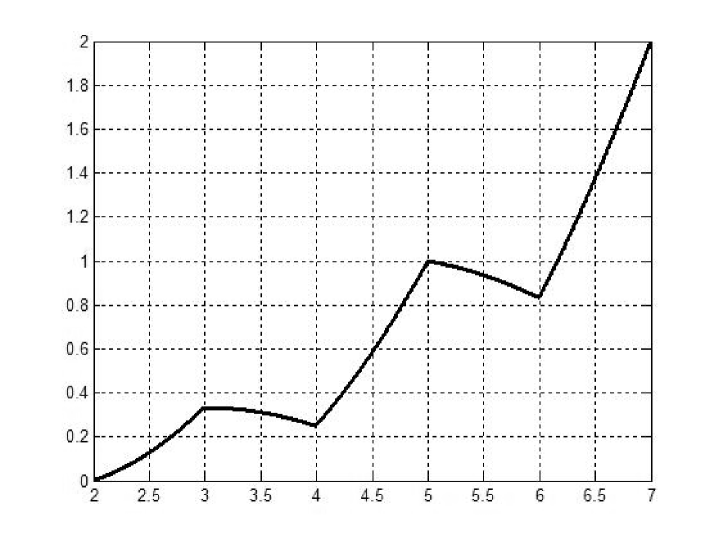
Figure 1: Graph of the function $D(\Lambda)$.

Let us consider some examples of a linear function $f(x)=\Lambda x,$ that illustrated the results of theorem 3.

Example 6.

1. Markov subpartition of $m=3$ subintervals: $I_{k,1}=[k-\frac{1}{2},k-\xi),$ $I_{k,2}=[k-\xi,k+\xi),$ $I_{k,3}=[k+\xi,k+\frac{1}{2}),$ $k\in Z.$
2. A system of two equations for $\xi$ and the value of slope $\Lambda:$

$$\Lambda\xi=\frac{1}{2},\qquad\Lambda\frac{1}{2}=2-\xi.$$

3. An equation for $\Lambda:$  $\Lambda^{2}-4\Lambda+1=0.$
4. A value of $\Lambda:$  $\Lambda=2+\sqrt{3}\approx 3.73.$
5. A value of $\xi:$  $\xi=\frac{2-\sqrt{3}}{2}\approx 0.13.$
6. A matrix $P(\lambda):$

$$P(\lambda)=\displaystyle\frac{1}{\Lambda}\left(\begin{array}[]{ccc}e^{-i\lambda}&1&e^{i\lambda}+e^{2i\lambda}\\ e^{-i\lambda}&1&e^{i\lambda}\\ e^{-i\lambda}+e^{-2i\lambda}&1&e^{i\lambda}\end{array}\right).$$

7. A value of greatest eigenvalue $z(\lambda)$ of matrix $P(\lambda):$
$z(\lambda)=\frac{1}{\lambda}(1+\cos\lambda+\sqrt{\cos^{2}\lambda+2\cos\lambda}).$
8. A value of deterministic diffusion coefficient:  $D=\frac{\sqrt{3}}{6}\approx 0.29.$
9. Values of densities $\alpha_{j}$ on subintervals $I_{k,j}:$  $\alpha_{1}=\alpha_{3}=\frac{2\sqrt{3}+3}{6}\approx 1.08,$   $\alpha_{2}=\frac{3+\sqrt{3}}{6}\approx 0.79.$

Example 7.

1. Markov subpartition of $m=3$ subintervals:
$I_{k,1}=[k-\frac{1}{2},k-\xi),$ $I_{k,2}=[k-\xi,k+\xi),$ $I_{k,3}=[k+\xi,k+\frac{1}{2}),$ $k\in Z.$
2. A system of two equations for $\xi$ and the value of slope $\Lambda:$

$$\Lambda\xi=\frac{3}{2},\,\,\,\qquad\Lambda\frac{1}{2}=3-\xi.$$

3. An equation for $\Lambda:$   $\Lambda^{2}-6\Lambda+3=0.$
4. A value of $\Lambda:$  $\Lambda=3+\sqrt{6}\approx 5.45.$
5. A value of $\xi:$  $\xi=\frac{3-\sqrt{6}}{2}\approx 0.28.$
6. A matrix $P(\lambda):$

$$P(\lambda)=\displaystyle\frac{1}{\Lambda}\left(\begin{array}[]{ccc}e^{-2i\lambda}&1+e^{i\lambda}+e^{-i\lambda}&e^{2i\lambda}+e^{3i\lambda}\\ e^{-2i\lambda}&1+e^{i\lambda}+e^{-i\lambda}&e^{2i\lambda}\\ e^{-2i\lambda}+e^{-3i\lambda}&1+e^{i\lambda}+e^{-i\lambda}&e^{2i\lambda}\end{array}\right).$$

7. An equation for greatest eigenvalue $z(\lambda)$ of matrix $P(\lambda):$
$\Lambda^{3}z^{3}-\Lambda^{2}z^{2}(1+2\cos\lambda+2\cos 2\lambda)-\Lambda z(1+2\cos\lambda)+1+2\cos\lambda=0.$
8. A value of deterministic diffusion coefficient:
$\displaystyle D=\frac{31\Lambda-16}{36\Lambda-24}\approx 0.89.$
9. Values of densities $\alpha_{j}$ on subintervals $I_{k,j}:$  $\alpha_{1}=\alpha_{3}=\frac{\sqrt{6}+2}{2}\approx 2.22,$   $\alpha_{2}=\frac{3+\sqrt{6}}{6}\approx 0.9.$

Example 8.

1. Markov subpartition of $m=3$ subintervals:
$I_{k,1}=[k-\frac{1}{2},k-\xi),$ $I_{k,2}=[k-\xi,k+\xi),$ $I_{k,3}=[k+\xi,k+\frac{1}{2}),$ $k\in Z.$
2. A system of two equations for $\xi$ and the value of slope $\Lambda:$

$$\Lambda\xi=\frac{3}{2},\,\,\,\qquad\Lambda\frac{1}{2}=2+\xi.$$

3. An equation for $\Lambda:$   $\Lambda^{2}-4\Lambda-3=0.$
4. A value of $\Lambda:$   $\Lambda=2+\sqrt{7}\approx 4.65.$
5. A value of $\xi:$   $\xi=\frac{\sqrt{7}-2}{2}\approx 0.32.$
6. A matrix $P(\lambda):$

$$P(\lambda)=\displaystyle\frac{1}{\Lambda}\left(\begin{array}[]{ccc}0&1+e^{i\lambda}+e^{-i\lambda}&e^{2i\lambda}\\ e^{-2i\lambda}&1+e^{i\lambda}+e^{-i\lambda}&e^{2i\lambda}\\ e^{-2i\lambda}&1+e^{i\lambda}+e^{-i\lambda}&0\end{array}\right).$$

7. An equation for greatest eigenvalue $z(\lambda)$ of matrix $P(\lambda):$
$-\Lambda^{3}z^{3}+\Lambda^{2}z^{2}(1+2\cos\lambda)+\Lambda z(1+2\cos 2\lambda(1+2\cos\lambda))+1+2\cos\lambda=0.$
8. A value of deterministic diffusion coefficient:
$\displaystyle D=\frac{9\Lambda+2}{13\Lambda-9}=\frac{479+107\sqrt{7}}{894}\approx 0.85.$
9. Values of densities $\alpha_{j}$ on subintervals $I_{k,j}:$  $\alpha_{1}=\alpha_{3}=\frac{1}{2}+\frac{1}{\sqrt{7}},$   $\alpha_{2}=\frac{1}{2}+\frac{1}{2\sqrt{7}}.$

Example 9.

1. Markov subpartition of $m=4$ subintervals:
$I_{k,1}=[k-\frac{1}{2},k-\xi),$ $I_{k,2}=[k-\xi,k),$ $I_{k,3}=[k,k+\xi),$ $I_{k,4}=[k+\xi,k+\frac{1}{2}),$ $k\in Z.$
2. A system of two equations for $\xi$ and the value of slope $\Lambda:$

$$\Lambda\xi=1,\,\,\,\qquad\Lambda\frac{1}{2}=1+\xi.$$

3. An equation for $\Lambda:$    $\Lambda^{2}-2\Lambda-2=0.$
4. A value of $\Lambda:$   $\Lambda=1+\sqrt{3}\approx 2.73.$
5. A value of $\xi:$  $\xi=\frac{\sqrt{3}-1}{2}\approx 0.37.$
6. A matrix $P(\lambda):$

$$P(\lambda)=\displaystyle\frac{1}{\Lambda}\left(\begin{array}[]{cccc}0&1&e^{i\lambda}&0\\ e^{-i\lambda}&1&e^{i\lambda}&0\\ 0&e^{-i\lambda}&1&e^{i\lambda}\\ 0&e^{-i\lambda}&1&0\end{array}\right).$$

7. A value of greatest eigenvalue $z(\lambda)$ of matrix $P(\lambda):$
$z(\lambda)=\frac{1}{\Lambda}(1+\sqrt{1+2\cos\lambda}).$
8. A value of deterministic diffusion coefficient:  $D=\frac{3-\sqrt{3}}{12}\approx 0.11.$
9. Values of densities $\alpha_{j}$ on subintervals $I_{k,j}:$   $\alpha_{1}=\alpha_{4}=\frac{3+\sqrt{3}}{6}\approx 0.79,$   $\alpha_{2}=\alpha_{3}=\frac{3+2\sqrt{3}}{6}\approx 1.08.$

Example 10.

1. Markov subpartition of $m=4$ subintervals:
$I_{k,1}=[k-\frac{1}{2},k-\xi),$ $I_{k,2}=[k-\xi,k),$ $I_{k,3}=[k,k+\xi),$ $I_{k,4}=[k+\xi,k+\frac{1}{2}),$ $k\in Z.$
2. A system of two equations for $\xi$ and the value of slope $\Lambda:$

$$\Lambda\xi=1,\,\,\,\qquad\Lambda\frac{1}{2}=2-\xi.$$

3. An equation for $\Lambda:$    $\Lambda^{2}-4\Lambda+2=0.$
4. A value of $\Lambda:$   $\Lambda=2+\sqrt{2}\approx 3.41.$
5. A value of $\xi:$  $\xi=\frac{2-\sqrt{2}}{2}\approx 0.29.$
6. A matrix $P(\lambda):$

$$P(\lambda)=\displaystyle\frac{1}{\Lambda}\left(\begin{array}[]{cccc}e^{-i\lambda}&1&e^{i\lambda}&e^{2i\lambda}\\ e^{-i\lambda}&1&e^{i\lambda}&0\\ 0&e^{-i\lambda}&1&e^{i\lambda}\\ e^{-i\lambda}&e^{-i\lambda}&1&e^{i\lambda}\end{array}\right).$$

7. A value of greatest eigenvalue $z(\lambda)$ of matrix $P(\lambda):$
$z(\lambda)=\frac{1}{\Lambda}(1+\cos\lambda+\sqrt{2-\sin^{2}\lambda}).$
8. A value of deterministic diffusion coefficient:  $D=\frac{1}{4}.$
9. Values of densities $\alpha_{j}$ on subintervals $I_{k,j}:$  $\alpha_{1}=\alpha_{4}=\frac{\sqrt{2}-1}{2}\approx 0.21,$   $\alpha_{2}=\alpha_{3}=\frac{2-\sqrt{2}}{2}\approx 0.29.$

Example 11.

1. Markov subpartition of $m=3$ subintervals:
$I_{k,1}=[k-\frac{1}{2},k-\xi_{2}),$ $I_{k,2}=[k-\xi_{2},k-\xi_{1}),$ $I_{k,3}=[k-\xi_{1},k+\xi_{1}),$ $I_{k,4}=[k+\xi_{1},k+\xi_{2}),$ $I_{k,5}=[k+\xi_{2},k+\frac{1}{2}),$ $k\in Z.$
2. A system of equations for $\xi$ and the value of slope $\Lambda:$

$$\Lambda\xi_{1}=\frac{3}{2},\,\,\,\qquad\Lambda\xi_{2}=2-\xi_{1},\,\,\,\qquad\Lambda\frac{1}{2}=2+\xi_{2}.$$

3. An equation for $\Lambda:$     $\Lambda^{3}-4\Lambda^{2}-4\Lambda+3=0.$
4. A value of $\Lambda:$  $\Lambda\approx 4.75.$
5. A value of $\xi:$  $\xi_{1}=\frac{3}{2\Lambda},\,\,\,\xi_{2}=\frac{4\Lambda-3}{2\Lambda^{2}}.$
6. A matrix $P(\lambda):$

$$P(\lambda)=\displaystyle\frac{1}{\Lambda}\left(\begin{array}[]{ccccc}0&0&1+e^{i\lambda}+e^{-i\lambda}&e^{2i\lambda}&0\\ e^{-2i\lambda}&0&1+e^{i\lambda}+e^{-i\lambda}&e^{2i\lambda}&0\\ e^{-2i\lambda}&0&1+e^{i\lambda}+e^{-i\lambda}&0&e^{2i\lambda}\\ 0&e^{-2i\lambda}&1+e^{i\lambda}+e^{-i\lambda}&0&e^{2i\lambda}\\ 0&e^{-2i\lambda}&1+e^{i\lambda}+e^{-i\lambda}&0&0\end{array}\right).$$

7. An equation for greatest eigenvalue $z(\lambda)$ of matrix $P(\lambda):$
$\Lambda^{5}z^{5}-\Lambda^{4}z^{4}(1+2\cos\lambda)-\Lambda^{3}z^{3}(1+2\cos\lambda(1+2\cos\lambda))-\Lambda^{2}z^{2}(1+2\cos\lambda+2\cos 2\lambda)-z+1+2\cos\lambda=0.$
8. A value of deterministic diffusion coefficient:  $\displaystyle D=\frac{81\Lambda^{2}+69\Lambda-55}{131\Lambda^{2}+99\Lambda-93}\approx 0.64.$
9. Values of densities $\alpha_{j}$ on subintervals $I_{k,j}:$  $\alpha_{1}=\alpha_{5}=\frac{\Lambda^{2}+4\Lambda-3}{4\Lambda(9-\Lambda)},$   $\alpha_{2}=\alpha_{4}=\frac{\Lambda^{2}+4\Lambda-3}{16(9-\Lambda)},$   $\alpha_{3}=\frac{5\Lambda^{2}-11\Lambda+6}{16(9-\Lambda)}.$

Example 12.

1. Markov subpartition of $m=6$ subintervals:
$I_{k,1}=[k-\frac{1}{2},k-\xi_{2}),$ $I_{k,2}=[k-\xi_{2},k-\xi_{1}),$ $I_{k,3}=[k-\xi_{1},k),$ $I_{k,4}=[k,k+\xi_{1}),$ $I_{k,5}=[k+\xi_{1},k+\xi_{2}),$ $I_{k,6}=[k+\xi_{2},k+\frac{1}{2}),$ $k\in Z.$
2. A system of equations for $\xi$ and the value of slope $\Lambda:$

$$\Lambda\xi_{1}=\xi_{2},\,\,\,\qquad\Lambda\xi_{2}=2-\xi_{1},\,\,\,\qquad\Lambda\frac{1}{2}=2+\xi_{1}.$$

3. An equation for $\Lambda:$    $\Lambda^{3}-4\Lambda^{2}+\Lambda-8=0.$
4. A value $\Lambda:$  $\Lambda\approx 4.22.$
5. A value $\xi:$  $\xi_{1}=\frac{2}{\Lambda^{2}+1},\,\,\,\xi_{2}=\frac{2\Lambda}{\Lambda^{2}+1}.$
6. A matrix $P(\lambda):$

$$P(\lambda)=\displaystyle\frac{1}{\Lambda}\left(\begin{array}[]{cccccc}0&1+e^{-i\lambda}&0&0&e^{i\lambda}+e^{2i\lambda}&0\\ 0&e^{-i\lambda}&1&0&e^{i\lambda}+e^{2i\lambda}&0\\ e^{-2i\lambda}&e^{-i\lambda}&1&0&e^{i\lambda}&e^{2i\lambda}\\ e^{-2i\lambda}&e^{-i\lambda}&0&1&e^{i\lambda}&e^{2i\lambda}\\ 0&e^{-i\lambda}+e^{-2i\lambda}&0&1&e^{i\lambda}&0\\ 0&e^{-i\lambda}+e^{-2i\lambda}&0&0&1+e^{i\lambda}&0\end{array}\right).$$

7. An equation for greatest eigenvalue $z(\lambda)$ of matrix $P(\lambda):$
$-\Lambda^{4}z^{4}+\Lambda^{3}z^{3}(1+2\cos\lambda)+\Lambda^{2}z^{2}(1+2\cos\lambda)+z(1+2\cos\lambda+2\cos 2\lambda+2\cos 3\lambda)+2+2\cos 2\lambda+4\cos\lambda\cos 2\lambda=0.$
8. A value of deterministic diffusion coefficient:  $\displaystyle D=\frac{5\Lambda^{2}+26\Lambda+22}{18\Lambda^{2}+18\Lambda+56}\approx 0.49.$
9. Values of densities $\alpha_{j}$ on subintervals $I_{k,j}:$  $\alpha_{1}=\alpha_{6}=\frac{\Lambda^{2}+1}{3\Lambda^{2}-8\Lambda+1},$   $\alpha_{2}=\alpha_{5}=\frac{\Lambda^{2}+2}{3\Lambda^{2}-8\Lambda+1},$   $\alpha_{3}=\alpha_{4}=\frac{\Lambda^{2}+\Lambda+5}{3\Lambda^{2}-8\Lambda+1}.$

Example 13.

1. Markov subpartition of $m=7$ subintervals:
$I_{k,1}=[k-\frac{1}{2},k-\xi_{3}),$ $I_{k,2}=[k-\xi_{3},k-\xi_{2}),$  $I_{k,3}=[k-\xi_{2},k-\xi_{1}),$ $I_{k,4}=[k-\xi_{1},k+\xi_{1}),$ $I_{k,5}=[k+\xi_{1},k+\xi_{2}),$ $I_{k,6}=[k+\xi_{2},k+\xi_{3})$, $I_{k,7}=[k+\xi_{3},k+\frac{1}{2})$ $k\in Z.$
2. A system of equations for $\xi$ and the value of slope $\Lambda:$

$$\Lambda\xi_{1}=\xi_{2},\qquad\Lambda\xi_{2}=\xi_{3},\qquad\Lambda\xi_{3}=\frac{1}{2},\qquad\Lambda\frac{1}{2}=2-\xi_{1}.$$

3. An equation for $\Lambda:$    $\Lambda^{4}-4\Lambda^{3}+1=0.$
4. A value of $\Lambda:$  $\Lambda\approx 3.968.$
5. A value of $\xi:$  $\xi_{1}=\frac{1}{2\Lambda^{3}},\,\,\,\xi_{2}=\frac{1}{2\Lambda^{2}},\,\,\,\xi_{3}=\frac{1}{2\Lambda}.$
6. A matrix $P(\lambda):$

$$P(\lambda)=\displaystyle\frac{1}{\Lambda}\left(\begin{array}[]{ccccccc}e^{-i\lambda}&1&0&0&0&0&e^{i\lambda}+e^{2i\lambda}\\ e^{-i\lambda}&0&1&0&0&0&e^{i\lambda}+e^{2i\lambda}\\ e^{-i\lambda}&0&0&1&0&0&e^{i\lambda}+e^{2i\lambda}\\ e^{-i\lambda}&0&0&1&0&0&e^{i\lambda}\\ e^{-i\lambda}+e^{-2i\lambda}&0&0&1&0&0&e^{i\lambda}\\ e^{-i\lambda}+e^{-2i\lambda}&0&0&0&1&0&e^{i\lambda}\\ e^{-i\lambda}+e^{-2i\lambda}&0&0&0&0&1&e^{i\lambda}\end{array}\right).$$

7. An equation for greatest eigenvalue $z(\lambda)$ of matrix $P(\lambda):$
$\Lambda^{4}z^{4}-\Lambda^{3}z^{3}(2+2\cos\lambda)+1=0.$
8. A value of deterministic diffusion coefficient:  $D=\frac{1}{4(\Lambda-3)}\approx 0.26.$
9. Values of densities $\alpha_{j}$ on subintervals $I_{k,j}:$  $\alpha_{1}=\alpha_{7}=\frac{\Lambda}{4(\Lambda-3)},$   $\alpha_{2}=\alpha_{6}=\frac{\Lambda}{4},$   $\alpha_{3}=\alpha_{5}=\frac{(\Lambda^{2}-3\Lambda-3)\Lambda}{4(\Lambda-3)},$   $\alpha_{4}=\frac{\Lambda^{2}}{4}-\frac{3}{4}-\frac{5}{2(\Lambda-3)}.$

The results of theorem 3 and above-considered examples allow us to give the following definition of deterministic diffusion of LDS (1)-(3).

Definition 6.

We say that the LDS (1)–(3) has a deterministic diffusion if, for any initial probability measure $\mu_{0}$ with bounded density, there exist a sequence of numbers $\sigma_{n}^{2}>0$ and $\xi_{n}$ and 1–periodic function $\alpha(x)\geq 0,$ $\int\limits_{-1/2}^{1/2}\,\alpha(x)\,dx=1,$ such that the sequence of measures $\mu_{n}=F^{n}\mu_{0}$, obtained from the initial measure by the $n$-fold action of the LDS, is asymptotically equivalent, as $n\rightarrow\infty$ to a sequence of measures with densities

$$\rho_{n}(x)=\frac{\alpha(x)}{\sigma_{n}\sqrt{2\pi}}e^{-\frac{(x-\xi_{n})^{2}}{2\sigma_{n}^{2}}}.$$

Remark 2.

The LDS (1)–(3) on the entire axis generates the associated DS $x_{n+1}=\hat{f}(x_{n})$ on the finite segment $[-\frac{1}{2},\frac{1}{2}),$ where the value of the function $\hat{f}(x_{n})$ is equal to the fractional part of $f(x),$ i.e., $\hat{f}(x_{n})=\{f(x)),$ and the function $\hat{f}$ maps the segment $[-\frac{1}{2},\frac{1}{2})$ into itself. We denote this DS, which is a compactification of the LDS, by CLDS. The function $\alpha(x)\geq 0$ in Definition 6 is the density of the invariant probability measure for the CLDS.

5 Deterministic Diffusion in the Case of Transportation in a Billiard Channel

The results of numerical experiments carried out in [2] demonstrate that the deterministic diffusion in long billiard channels is anomalous. There are different theoretical models of this type of diffusion transport in long channels. One of these models can be found in [1]. The essence of this model can be described as follows:

Consider a long billiard channel with boundaries in the form of periodically repeated arcs slightly distorting the straight lines of boundaries. Assume that the upper boundary of the channel is symmetric to the lower boundary. Then the trajectory of motion of a billiard ball regarded as a material point obeying the ideal law of reflections from both boundaries can be studied in a channel of half width with symmetric reflections of the trajectory in the upper part of the channel into its lower part relative to the straight middle line of the channel. Hence, the reflections from this middle line can be regarded as ideal.

We approximately assume that the reflection from the lower part of the distorted boundary is realized in its linear approximation. However, the normal $\nu$ to the surface of actual reflection does not coincide with normal to the rectilinear approximation of the channel and is described by a known function periodic along the axis of the channel. Assume that $x_{n-1},$  $x_{n},$ and $x_{n+1}$ are the abscissas of points of three consecutive reflections of the billiard ball and that the vector $\nu(x_{n})$ makes an angle $\alpha(x_{n})$ with the normal to the surface (see Fig. 2). Then the analysis of the ideal reflection at the point $x_{n}$ leads to the equality of the angle of incidence $\varphi_{n}$ and the angle of reflection $\psi_{n}$ relative to the vector $\nu.$ It is clear that $\frac{x_{n}-x_{n-1}}{h}=\tan(\varphi-\alpha)$ and $\frac{x_{n+1}-x_{n}}{h}=\tan(\psi+\alpha).$ Hence,

$$\frac{x_{n+1}-x_{n}}{h}=\frac{\frac{x_{n+1}-x_{n}}{h}+\tan(2\alpha)}{1-\tan(2\alpha)\cdot\frac{x_{n+1}-x_{n}}{h}}.$$ (23)

For large $h,$ we get the following approximate relation from (23):

$$x_{n+1}-x_{n}=x_{n}-x_{n-1}+h\tan(2\alpha(x_{n})).$$

Figure 2: Reflections of the billiard ball in a channel of half width.

Let the function $f(x)=\tan(2\alpha x)$ be periodic in $x$ with period 1. Then we arrive at the following model of a trajectory in the billiard channel:

$$x_{n+1}-x_{n}=x_{n}-x_{n-1}+f(x_{n}).$$ (24)

The dynamical system (24) is a two-dimensional dynamical system discrete in time which generalizes the dynamical system (1). The initial conditions for $x_{0}$ and $x_{1}$ are assumed to be given. Let $x_{0}=0$ and let $x_{1}\in I_{k}=[k-\frac{1}{2},k+\frac{1}{2}).$ Equation (24) can be represented in the equivalent form as follows:

$$x_{n+1}=x_{1}\cdot n+\sum\limits_{k=1}^{n}\,(n+1-k)f(x_{k}).$$ (25)

Assume that the function $f(x)=\Lambda\cdot\{x)$ in Eq. (25) is linear with respect to the fractional part of the argument. Then, for $\Lambda>1$ and $x_{1}$ uniformly distributed over the interval $I_{k},$ the terms in (25) can be regarded uniformly distributed independent random variables. This leads to the normal distribution of $x_{n+1}$ with variance equal to the sum of variances of all terms in (25).

Hence, the variance of the distribution of $x_{n+1}$ is equal to $\displaystyle\sigma^{2}=\frac{1}{12}n^{2}+\frac{\Lambda^{2}}{12}\frac{n(n+1)(2n+1)}{6}$ and nonlinearly depends on $n\rightarrow\infty.$ The deterministic diffusion in this billiard strip is anomalous. Thus, there are two factors leading to the anomaly of the deterministic diffusion, namely, the quadratic dependence of the variance on distribution of the initial values even for the ideal billiard and the growth of coefficients of the terms in sum (25) leading to the cubic dependence of the variance of $x_{n+1}$ on $n.$

We now make an important remark. We have studied the distribution of positions of the billiard ball after $n\rightarrow\infty$ reflections. From the physical point of view, it is more important to get the distribution of the abscissas of billiard balls for large values of time $t$ because, for the the same period of time, the billiard ball makes different numbers of reflections for different trajectories.

In the ordinary billiards, the time between two successive collisions is proportional to the covered distance. However, in the model of bouncing ball [13] over an irregular surface, the time between two consecutive collisions is maximal if the points of consecutive reflections coincide. The problem of investigation of the anomalous deterministic diffusion in billiard channels as $t\rightarrow\infty$ is of significant independent interest.

Note that the Gaussian density in the case of ordinary diffusion is the Green function of the Cauchy problem for the partial differential equation

$$\frac{\partial u}{\partial t}-D\Delta u=0.$$

In the investigation of anomalous diffusion, we consider a differential equation with fractional derivatives. Equations of this kind are studied in numerous works (see [11] and the references therein).

Acknowledgments

The authors express their gratitude to Prof. A. Katok for a remarkable course of lectures on the contemporary theory of dynamical systems delivered in May, 2014 in Kiev and for the informal discussions which stimulated the authors to write this paper.

References

- [1] S. Albeverio, G. Galperin, I. Nizhnik and L. Nizhnik: Generalized billiards inside an infinite strip with periodic laws of reflection along the strip’s boundaries, (2004), Preprint Nr 04-08-154, pp. 28, BiBoS, Universität Bielefeld, Regular and Chaotic Dynamics 10 (3) (2005), 285-306.
- [2] D. Alonso, A. Ruiz, I. de Vega: Transport in polygonal billiards, Physica D, 187 (2004), pp. 184-199.
- [3] R. N. Bhattacharya, R. Ranga Rao: Normal Approximation and Asymptotic Expansions, 1976.
- [4] P. Cvitanović, R. Artuso, R. Mainieri, G.Tanner, G. Vattay, N. Whelan, A. Wirzba: Classical and Quantum Chaos (2004), http://www.nbi.dk/ChaosBook/
- [5] W. Feller: An Introduction to Probability Theory and its Applications, 1968.
- [6] B.V. Gnedenko, A.N. Kolmogorov: Limit distributions for sums of independent random variables, Addison-Wesley Mathematics Series, Cambridge: Addison-Wesley Publishing Company, IX, 1954.
- [7] B. Hasselblatt, A.Katok: A first course in dynamics with a panorama of recent developments, Cambridge University press, 2003.
- [8] A. Katok, B. Hasselblatt: Introduction ot the Modern Theory of Dynamical Systems, Cambridge University press, Cambridge, 1995.
- [9] R. Klages: Microscopic Chaos, Fractals and Transport in Nonequilibrium Statistical Mechanics, World Scientific, 2007.
- [10] R. Klages, G.Radons, I.Sokolov (Eds): Anomalous transport, Wiley-VCH, 2008.
- [11] A. N. Kochubei: Cauchy problem for fractional diffusion-wave equations with variable coefficients // 2013, arXiv: 1308.6452v1, 31 p., http://arxiv.org/pdf/1308.6452v1.pdf, Applicable Analysis, vol 93, issue 10, 2211-2242, 2014.
- [12] N. Korabel, R. Klages: Fractality of deterministic diffusion in the nonhyperbolic climbing sine map, CHAOTRAN proceedings in Physica D 187, (2004), 66–88.
- [13] L. Matyas, R. Klages: Irregular diffusion in the bouncing ball billiard, Physica D, 187 (2004), pp. 165-183.
- [14] A.N. Sharkovsky, S.F. Kolyada, A.G. Sivak, V.V. Fedorenko, Dynamics of one-dimensional maps [Translated from Russian], Mathematics and its Applications, vol. 407, Kluwer Academic Publ., Dordrecht, 1997.