The Origin of the Hot Gas in the Galactic Halo: Testing Galactic Fountain Models’ X-ray Emission

Abstract

We test the X-ray emission predictions of galactic fountain models against XMM-Newton measurements of the emission from the Milky Way’s hot halo. These measurements are from 110 sight lines, spanning the full range of Galactic longitudes. We find that a magnetohydrodynamical simulation of a supernova-driven interstellar medium, which features a flow of hot gas from the disk to the halo, reproduces the temperature but significantly underpredicts the 0.5–2.0 keV surface brightness of the halo (by two orders of magnitude, if we compare the median predicted and observed values). This is true for versions of the model with and without an interstellar magnetic field. We consider different reasons for the discrepancy between the model predictions and the observations. We find taking into account overionization in cooled halo plasma, which could in principle boost the predicted X-ray emission, is unlikely in practice to bring the predictions in line with the observations. We also find that including thermal conduction, which would tend to increase the surface brightnesses of interfaces between hot and cold gas, would not overcome the surface brightness shortfall. However, charge exchange emission from such interfaces, not included in the current model, may be significant. The faintness of the model may also be due to the lack of cosmic ray driving, meaning that the model may underestimate the amount of material transported from the disk to halo. In addition, an extended hot halo of accreted material may be important, by supplying hot electrons that could boost the emission of the material driven out from the disk. Additional model predictions are needed to test the relative importance of these processes in explaining the observed halo emission.

1. INTRODUCTION

X-ray observations show that the halo of our galaxy contains hot, diffuse plasma. This plasma is observed both in emission, as a component of the $\sim$0.1–1 keV soft X-ray background (SXRB; e.g., Kuntz & Snowden, 2000; Yoshino et al., 2009; Henley et al., 2010; Henley & Shelton, 2013), and in absorption, in high-resolution X-ray spectra of bright background sources (Nicastro et al., 2002; Rasmussen et al., 2003; McKernan et al., 2004; Fang et al., 2006; Bregman & Lloyd-Davies, 2007; Yao & Wang, 2007; Yao et al., 2009; Hagihara et al., 2010; Gupta et al., 2012). Although the Milky Way’s hot halo is well studied observationally, the details of the origin of this hot plasma remain uncertain. Understanding the relative importance to the hot halo of supernova (SN) driven outflows from the disk and inflows from the intergalactic medium is a key part of understanding the functioning of the Galaxy and its interaction with its environment.

In Henley et al. (2010, hereafter H10), we tested models of the hot halo plasma against 26 XMM-Newton observations of the high-latitude SXRB, by comparing the observed temperatures and emission measures of the halo with the distributions predicted by different physical models. H10’s analysis favored SN-driven galactic fountains (Joung & Mac Low, 2006, hereafter JM06) as a major, possibly dominant, source of the hot halo plasma observed in emission, although these fountain models tended to overpredict the halo temperature. Additional support for the heating of the halo by disk SNe comes from the observation that some models of the halo’s global gas distribution (constrained by various observational data) imply that the hot halo may be convectively unstable (Henley & Shelton, 2014). However, H10 were unable to rule out the possibility that an extended halo of accreted material also contributes to the emission (Crain et al., 2010).

In this paper, we further examine the X-ray predictions of galactic fountain models, in the light of two developments since H10. First, we use a much larger set of measurements of the Galactic halo emission. Henley & Shelton (2013, hereafter HS13) measured the halo X-ray emission on 110 high-latitude XMM-Newton sight lines, an approximately fourfold increase over H10. This is the largest set of measurements of the halo X-ray emission with CCD-resolution spectra assembled to date. Furthermore, these observations span the full range of Galactic longitudes, whereas H10’s data set was restricted to $l=120\arcdeg$–240°. See Section 2 for a description of the observational data. (Note that HS13 discussed the energetics of galactic outflows versus extragalactic accretion as sources of the observed X-ray emission, but were unable to distinguish between these two scenarios: both SNe and infall provide more than enough energy to power the observed emission, and either process could plausibly explain the observed variation of the surface brightness on the sky.)

Second, it has been discovered that the JM06 fountain model included an unphysical inflow of hot gas from the vertical boundaries that adversely affected the model’s X-ray predictions (see Section 3). We therefore examine a new model of the SN-driven interstellar medium (ISM), in which there is no such hot inflow (Hill et al., 2012, hereafter H12). In addition, these newer simulations include results obtained with a non-zero interstellar magnetic field. See Section 3 for a description of these ISM models.

Section 4 describes how we obtained the X-ray predictions from the ISM models. We present the results of the comparison of the model predictions with the observations in Section 5. We discuss the results in Section 6, and conclude with a summary in Section 7.

2. OBSERVATIONS

We use HS13’s measurements of the Galactic halo X-ray emission. They measured this emission on 110 high-latitude XMM-Newton sight lines, selected from an all-sky XMM-Newton survey of the SXRB (Henley & Shelton, 2012). HS13 applied various filters to Henley & Shelton’s (2012) observations in order to minimize the contamination from charge exchange (CX) emission from within the solar system, a time-variable contaminant of SXRB spectra (Cravens et al., 2001; Wargelin et al., 2004; Snowden et al., 2004; Koutroumpa et al., 2007; Fujimoto et al., 2007; Henley & Shelton, 2008; Ezoe et al., 2010; Carter et al., 2011). In addition, HS13 excluded certain features from their sample (the Scorpius-Centaurus superbubble, the Eridanus Enhancement, and the Magellanic Clouds). The HS13 data set contains measurements for $\sim$4 times as many sight lines as H10’s data set, spanning the full range of Galactic longitudes. Here we give a brief overview of HS13’s spectral modeling method and their halo results; see HS13 for more details, and for a comparison of their results with those from other recent studies of the SXRB.

HS13 analyzed the SXRB spectrum for each sight line with a standard SXRB model, with components representing the foreground, Galactic halo, and extragalactic background emission. The foreground emission was constrained using shadowing data from the ROSAT All-Sky Survey (Snowden et al., 2000). For all but one sight line, HS13 used a single-temperature ($1T$) collisional ionization equilibrium (CIE) plasma model to model the halo emission, obtaining the X-ray temperature and emission measure for the halo on each sight line. For the remaining sight line, HS13 added another, hotter component (with temperature $T\sim 11\times 10^{6}~{}\mbox{K}$), in order to model excess emission in the observed spectrum around $\sim$1 keV (see their Section 3.1.2). For that sight line, we use the results for the cooler component ($T\sim 2\times 10^{6}~{}\mbox{K}$).

HS13 detected emission from $\sim$$(\mbox{2--3})\times 10^{6}~{}\mbox{K}$ halo plasma on 87 out of 110 sight lines (79%), with a median temperature of $2.2\times 10^{6}~{}\mbox{K}$, and a typical intrinsic 0.5–2.0 keV surface brightness of $(\mbox{1.1--2.3})\times 10^{-12}~{}\mbox{erg}\ \mbox{cm}^{-2}\ \mbox{s}^{-1}\ \mbox{deg}^{-2}$. On the remaining 23 sight lines, HS13 give upper limits for the halo surface brightness.

Henley et al. (2014) compared a subset of HS13’s results with a measurement of the Galactic halo emission from an XMM-Newton observation of a compact shadowing cloud, G225.60$-$66.40. The good agreement between their measurement and that from the nearest HS13 sight line led Henley et al. (2014) to conclude that HS13’s measurements are not subject to systematic errors, and can confidently be used to test models of the halo emission.

3. GALACTIC FOUNTAIN MODELS

The JM06 and H12 SN-driven ISM simulations were carried out using Flash, a parallelized Eulerian hydrodynamical code with adaptive mesh refinement (AMR). In each case, the model domain was a tall thin box extending to $z=\pm z_{\mathrm{max}}$, with periodic boundary conditions on the vertical sides, and zero-gradient boundary conditions on the upper and lower surfaces. The model domain was initialized with gas in hydrostatic equilibrium. This gas was then heated and stirred stochastically by Type Ia and core collapse SN explosions, each with a frequency and $z$ distribution appropriate for the Milky Way in the vicinity of the Sun. Each SN injected $10^{51}~{}\mbox{erg}$ of energy into a small region of the grid. 60% of the core collapse SNe occurred in clusters of seven to 40 explosions, while the remaining SNe occurred in isolation. The gas in the model domain was also subject to radiative cooling, and to diffuse heating representing photoelectric heating of dust grains. The simulations were run at least long enough to eradicate the initial conditions. From our point of view, the most important feature of these ISM models is that the SN heating drives a fountain of hot ($\gtrsim$$10^{6}~{}\mbox{K}$) X-ray-emissive gas into the halo. For more details of the models, see JM06 and H12.

H10 tested the JM06 ISM model, which was carried out in a $0.5\times 0.5\times 10~{}\mbox{kpc}^{3}$ model domain, with $z_{\mathrm{max}}=5~{}\mbox{kpc}$. H10 found that the X-ray emission measures predicted by this model were in good agreement with their observations, leading them to conclude that galactic fountains are a major, possibly dominant, contributor to the hot X-ray emission in the XMM-Newton band (as noted in the Introduction). However, the JM06 model overpredicted the observed X-ray temperature.

It has subsequently been discovered that the boundary conditions at the upper and lower boundaries of the JM06 model domain led to an unphysical inflow of hot, high-pressure gas into the domain (Mac Low et al. 2012; Joung et al. 2012; H12). Early in the simulation, while the initial conditions were still being eradicated, hot gas from SNe moved upward through and eventually off the domain, causing the ghost cells just off the domain to be set to a high-temperature, high-pressure state. Subsequent radiative cooling caused the halo pressure to drop, causing material to be drawn into the model domain. The state of this inflowing material was determined by the state of the ghost cells, leading to a hot, high-pressure inflow. This inflow adversely affected the X-ray predictions derived from the JM06 model.

The newer H12 model used outflow-only boundary conditions, and was carried out in a much larger domain—$1\times 1\times 40~{}\mbox{kpc}^{3}$, with $z_{\mathrm{max}}=20~{}\mbox{kpc}$—and so does not suffer from the unphysical inflow problem of the JM06 model. There are a few additional differences from the JM06 model. First, the Type Ia (core collapse) SN rate was slightly higher (lower) than that used in JM06, though otherwise the SN heating was the same. Second, the grid initialization was slightly different—JM06 initialized their entire domain with gas at $10^{4}~{}\mbox{K}$, whereas H12 initialized their domain with gas at $1.15\times 10^{4}$ and $1.15\times 10^{6}$ below and above $|z|\approx 1~{}\mbox{kpc}$, respectively (the pressure was continuous across the interface). Also, H12 employed a higher gas surface mass density than JM06: 13.2 versus 7.5 $M_{\odot}$ $\mbox{pc}^{-2}$. Finally, H12 ran versions of their model that included a magnetic field—here, we examine versions with (model bx50) and without (model bx0) a magnetic field. In model bx50, the magnetic field was initially horizontal and uniform in the $xy$ plane, with a magnitude of 6.5 $\mu\mbox{G}$, but decreased with height such that the ratio of magnetic and gas pressures was constant. Note that the radiative cooling and diffuse heating were incorrectly applied in the original H12 simulations, but corrected models were described in their erratum. Here, we use results from the corrected simulations.

It should be noted that HS13 found that the halo emission measure tends to increase toward the inner Galaxy ($l=0\arcdeg$). However, because the models’ domains are tall thin boxes, we are unable to determine how the model predictions would vary with Galactic longitude or latitude. Instead, we test how well the models can reproduce the overall distributions of observed halo temperatures and surface brightnesses.

4. CHARACTERIZING THE FOUNTAIN MODEL X-RAY EMISSION

Table 1Observed and Predicted Halo Temperatures and Surface Brightnesses, and Predicted Hot Gas Properties

									Properties of hot ($T\geq 10^{6}~{}\mbox{K}$) gas
	Obs. or Model	Time	Temperature			$S_{0.5-2.0}$			$\langle n_{\mathrm{e}}\rangle$			$\langle n_{\mathrm{e}}^{2}\rangle^{1/2}$			$L$
		(Myr)	($10^{6}~{}\mbox{K}$)						($10^{-3}~{}\mbox{cm}^{-3}$)			($10^{-3}~{}\mbox{cm}^{-3}$)			(kpc)
	(1)	(2)	(3)			(4)			(5)			(6)			(7)
1	Observations	$\cdots$	2.22	(2.01,	2.64)	1.07	(0.50,	1.53)	$\cdots$			$\cdots$			$\cdots$
2	H12 bx0	85	1.72	(1.19,	2.38)	0.016	(0.002,	0.062)	0.43	(0.19,	0.79)	0.55	(0.28,	1.02)	0.21	(0.10,	0.36)
3	H12 bx0	135	1.67	(1.10,	2.34)	0.006	(0.000,	0.031)	0.35	(0.15,	0.66)	0.45	(0.17,	0.85)	0.16	(0.04,	0.34)
4	H12 bx0	185	1.98	(1.62,	2.50)	0.020	(0.011,	0.068)	0.11	(0.09,	0.13)	0.15	(0.12,	0.25)	3.22	(2.91,	3.50)
5	H12 bx0	235	1.74	(1.33,	2.73)	0.012	(0.003,	0.035)	0.042	(0.036,	0.050)	0.078	(0.046,	0.123)	7.98	(7.05,	8.94)
6	H12 bx0	285	2.22	(1.77,	2.59)	0.023	(0.010,	0.058)	0.055	(0.043,	0.070)	0.098	(0.064,	0.150)	7.09	(5.32,	9.98)
7	H12 bx0	335	1.88	(1.68,	2.17)	0.010	(0.006,	0.040)	0.037	(0.035,	0.044)	0.059	(0.040,	0.112)	9.76	(8.29,	11.17)
8	H12 bx50	85	1.28	(0.93,	1.96)	0.001	(0.000,	0.015)	0.073	(0.047,	0.160)	0.10	(0.05,	0.36)	0.46	(0.19,	0.93)
9	H12 bx50	135	1.35	(1.01,	2.03)	0.004	(0.001,	0.035)	0.13	(0.10,	0.20)	0.17	(0.11,	0.40)	0.63	(0.43,	0.89)
10	H12 bx50	185	1.52	(1.02,	2.17)	0.005	(0.001,	0.029)	0.098	(0.040,	0.140)	0.15	(0.09,	0.29)	1.11	(0.70,	1.59)
11	H12 bx50	235	1.86	(1.35,	2.78)	0.015	(0.002,	0.048)	0.037	(0.025,	0.056)	0.11	(0.04,	0.18)	4.14	(3.64,	4.88)
12	H12 bx50	285	1.92	(1.61,	2.79)	0.012	(0.003,	0.041)	0.021	(0.018,	0.027)	0.066	(0.041,	0.109)	9.36	(9.07,	9.66)
13	H12 bx50	335	1.93	(1.60,	2.63)	0.011	(0.002,	0.046)	0.017	(0.014,	0.022)	0.060	(0.026,	0.111)	11.06	(9.66,	12.03)

Note. — For each quantity, we have tabulated the median value, followed by the lower and upper quartiles in parentheses. For the model predictions, these quartiles were calculated from the sets of values obtained from the 242 model sight lines that we examined at each model epoch. Columns 3 and 4 contain halo temperatures and surface brightnesses, respectively. Columns 5–7 contain the mean electron densities, the r.m.s. electron densities, and the path lengths of the hot gas along the model sight lines, respectively.

As in H10, for a given model epoch we calculated halo X-ray spectra for 242 vertical sight lines, looking upward and downward from the Galactic midplane. The vantage points for these sight lines were arranged in an $11\times 11$ grid in the Galactic midplane, with grid spacings of $\approx$98 pc. We used the Raymond & Smith (1977) spectral code (updated by J. C. Raymond & B. W. Smith, 1993, private communication with R. J. Edgar) to calculate the X-ray spectra, assuming that the plasma is in CIE and is optically thin. We excluded material within 100 pc of the midplane from the emission calculations, as such material is not in the halo. Note that the SXRB model used in the observational analysis (HS13) included a foreground component (in addition to the halo component, the results for which we use here; Section 2). This foreground component accounted for the observed emission from within $\sim$100 pc of the midplane.

The true halo emission is likely from plasma with a range of temperatures; in the observational analysis, this emission was characterized with a $1T$ plasma model (HS13). Similarly, the emission predicted by the fountain models that we are examining here is from plasma with a range of temperatures. Therefore, to ensure a like-with-like comparison of the models with the observations, we characterized the predicted X-ray emission by creating synthetic XMM-Newton observations of the SXRB, and then analyzing the resulting spectra with the same SXRB model used in the observational analysis. This method is described in full in H10; here we give an overview, and point out the differences from H10.

For each model sight line, we combined the predicted halo X-ray emission with models for the foreground emission, the extragalactic background, the instrumental fluorescence lines, and residual soft proton contamination (HS13). We folded the resulting spectrum through the XMM-Newton response function and added Poissonian noise corresponding to a typical field of view and exposure time from HS13. The simulations also took into account the XMM-Newton quiescent particle background. We simulated a MOS1 and a MOS2 spectrum for each model sight line, each of which we grouped such that there were at least 25 counts per bin (as in HS13). We then fitted the grouped spectra with the input SXRB model, but with the halo component replaced with a $1T$ CIE plasma model. We use the resulting best-fit $1T$ halo model to calculate the intrinsic 0.5–2.0 keV surface brightness, $S_{0.5-2.0}$. Thus, for each model sight line, we obtained an X-ray temperature and surface brightness which characterize the predicted X-ray spectrum, and which can be compared with the observed temperatures and surface brightnesses. Note that the model surface brightnesses obtained in this way were typically $\sim$20–40% lower than those obtained directly from the model spectra. This is likely because the $1T$ model used in the fitting cannot always accurately capture the entire model spectrum, calculated from a multitemperature plasma.

We used the same foreground model as in H10, but a different model for the extragalactic background. H10 used a single unbroken power-law (Chen et al., 1997), whereas we used the model from HS13: a double broken power-law (Smith et al., 2007) rescaled to match the expected surface brightness of the sources that fell below the source removal flux threshold (Moretti et al., 2003; Hickox & Markevitch, 2006). This alteration in the extragalactic model resulted in a change in the typical level of soft proton contamination; we adjusted our input model accordingly. The source removal flux threshold used in HS13 is lower than that used by H10, resulting in more of the XMM-Newton field of view being excluded in the observational analysis. We therefore lowered the assumed field of view for the simulated observations from 480 to 410 arcmin². However, we kept the assumed exposure time at 15 ks.

In order to ensure that the simulated spectra had adequate signal-to-noise to constrain the $1T$ halo model, we rescaled the input halo spectra such that they had a specified surface brightness. We undid this rescaling at the end, by dividing the output emission measure by the same factor that was used to multiply the input spectrum. In H10, we rescaled the spectra to give a 0.4–2.0 keV surface brightness of $2.06\times 10^{-12}~{}\mbox{erg}\ \mbox{cm}^{-2}\ \mbox{s}^{-1}\ \mbox{deg}^{-2}$. Here, we found that the X-ray temperatures resulting from this procedure may depend weakly on the assumed surface brightness used to rescale the spectra. We therefore used three different values to rescale the spectra: 0.5–2.0 keV surface brightnesses of $1.14\times 10^{-12}$, $1.54\times 10^{-12}$, and $2.34\times 10^{-12}~{}\mbox{erg}\ \mbox{cm}^{-2}\ \mbox{s}^{-1}\ \mbox{deg}^{-2}$ (these are the quartiles for sight lines on which $\sim$$(\mbox{2--3})\times 10^{6}~{}\mbox{K}$ emission is detected; HS13, Table 2).

We subjected the halo and extragalactic components of the model to interstellar absorption. The assumed column density does not strongly affect the results, but here too we decided to use the quartiles from HS13: $1.26\times 10^{20}$, $1.63\times 10^{20}$, and $2.12\times 10^{20}~{}\mbox{cm}^{-2}$ (cf. $1.7\times 10^{20}~{}\mbox{cm}^{-2}$ in H10). Thus, each model sight line was characterized a total of nine times. For the comparison with the observations, we first combined the results obtained with the different rescaling surface brightnesses and column densities.

5. RESULTS

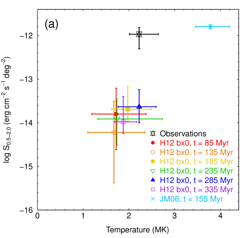
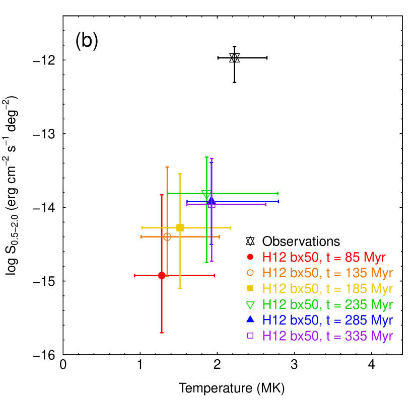
Figure 1.— Comparison of the H12 (a) bx0 and (b) bx50 fountain model predictions with the HS13 halo observations in the temperature–surface-brightness plane. The observations are plotted in black, while the other colors represent different epochs of the H12 models. For each plotted data point, the symbol indicates the medians, while the error bars indicate the lower and upper quartiles. For the observations, only sight lines on which the halo temperature was free to vary are included in the temperature data (see HS13). The observed surface brightnesses have been latitude-corrected assuming a plane parallel halo geometry, and non-detections are included at their best-fit values. In the bx0 plot, we also show results for one epoch of the JM06 model (the latest epoch examined by H10).

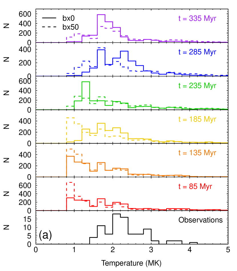
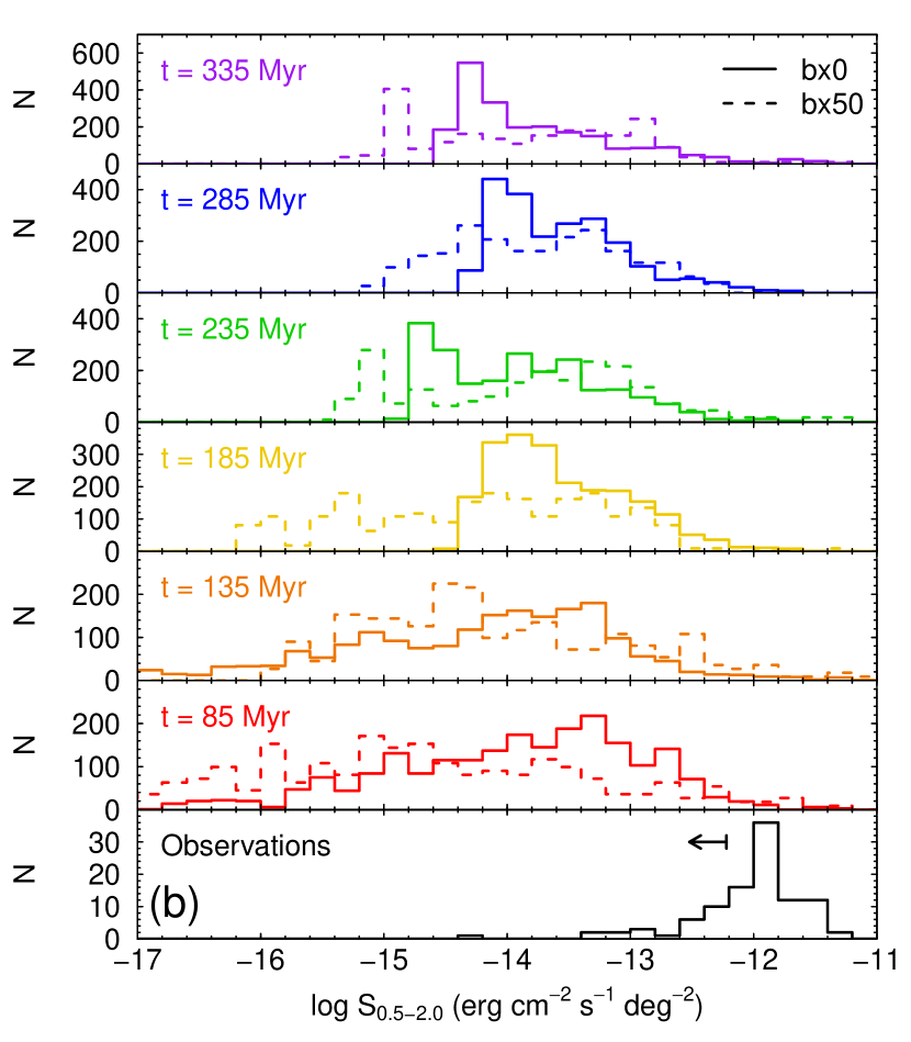
Figure 2.— Comparison of the observed and predicted distributions of halo (a) temperatures and (b) 0.5–2.0 keV surface brightnesses. In each plot, the bottom panel shows the observed distribution (HS13). Similarly to Figure 1, only sight lines on which the halo temperature was free to vary are included in the observed temperature distribution, and the observed surface brightness distribution shows the latitude-corrected values with non-detections included at their best-fit values. The arrow in the bottom panel of plot (b) indicates the median upper limit on the latitude-corrected surface brightness from the sight lines on which halo emission was not detected. In the other panels, the solid and dashed histograms show the predicted distributions from different epochs of the H12 bx0 and bx50 models, respectively. The colors representing the different model epochs match those used in Figure 1.

Figure 1 compares the X-ray predictions of the H12 fountain model with HS13’s halo observations in the temperature–surface-brightness plane. We show predictions from several different epochs of the models (a) without and (b) with a magnetic field (models bx0 and bx50, respectively). For comparison with H10, Figure 1(a) also shows predictions from a single epoch of the JM06 model (the latest epoch examined by H10).

Figure 2 compares the predicted temperature and surface brightness distributions of the H12 models with the observed distributions. Again, we show results from several different epochs of models bx0 and bx50. The observed and predicted halo temperatures and surface brightnesses are summarized in columns 3 and 4 of Table 1, respectively. The observations are in row 1, while the predictions from models bx0 and bx50 are in rows 2–7 and 8–13, respectively. Table 1 also summarizes the properties of the hot ($T\geq 10^{6}~{}\mbox{K}$) gas from each epoch of the models—columns 5–7 contain the mean electron densities, $\langle n_{\mathrm{e}}\rangle$, the r.m.s. electron densities, $\langle n_{\mathrm{e}}^{2}\rangle^{1/2}$, and the path lengths, $L$, of this gas along the model sight lines, respectively. Note that the r.m.s. electron density is more useful than the mean electron density for interpreting the X-ray emission predictions, since the emission measure $\mathcal{E}=\langle n_{\mathrm{e}}^{2}\rangle L$.

The predictions from model bx0 appear to undergo a slight oscillation in the temperature–surface-brightness plane. The median predicted X-ray temperature and surface brightness oscillate with peak-to-peak amplitudes of $\sim$$0.3\times 10^{6}~{}\mbox{K}$ and $\sim$0.3 dex, respectively, with a period of $\sim$100 Myr. This oscillation may be related to the “bouncing” of the halo material reported by H12.

At the earliest epochs of the bx0 model shown here, the r.m.s. density of the hot gas is relatively high ($\sim$$5\times 10^{-4}~{}\mbox{cm}^{-3}$) and the path length through this gas is relatively short ($\sim$0.2 kpc). At later epochs, the density is lower ($\sim$$1\times 10^{-4}~{}\mbox{cm}^{-3}$) but the path length much longer (up to $\sim$10 kpc). However, these changes are such that $\mathcal{E}$ remains the same within a factor of $\sim$2 ($\sim$$5\times 10^{-5}$ and $\sim$$1\times 10^{-4}~{}\mbox{cm}^{-6}\ \mbox{pc}$, respectively, using the above-quoted densities and path lengths). (As an aside, we note that the median r.m.s. density and path length from the sight lines through the JM06 model are $9\times 10^{-4}~{}\mbox{cm}^{-3}$ and 4 kpc, respectively, for the epoch plotted in Figure 1(a). Comparing these values with those from the later epochs of the H12 bx0 model implies that the main effect of the unphysical inflow in the JM06 model is to increase the density of the hot halo gas by an order of magnitude, and hence the X-ray surface brightness by two orders of magnitude.)

The predictions from model bx50 do not oscillate, but instead there is a general increase in the predicted X-ray temperatures and surface brightnesses from $t=85$ to $t=235~{}\mbox{Myr}$—the medians increase by $\sim$$0.6\times 10^{6}~{}\mbox{K}$ and an order of magnitude, respectively, over this time period. The increase in brightness is mainly due to an order-of-magnitude increase in the path length through the hot gas, due to a shock being driven upward through the halo. The path length through the hot gas continues to increase beyond $t=235~{}\mbox{Myr}$, but more slowly than at earlier epochs, as the shock slows down. The r.m.s. density of the hot gas in the bx50 model decreases from $t=135~{}\mbox{Myr}$ onward, because the hot gas extends to greater heights, and thus includes lower-density gas. After $t=235~{}\mbox{Myr}$, the model bx50 X-ray predictions are fairly steady, although there is some variation in the shapes of the predicted distributions. At these later epochs of the bx50 model, its predictions are similar to those from model bx0.

Now that we have understood the H12 X-ray predictions in terms of the physical properties of the hot gas in the model domains, we can compare these predictions with the HS13 halo measurements. The models generally underpredict the median observed halo temperature by $\sim$10–20%, although the predictions and observations agree within the observed sight line-to-sight line temperature variation. However, the models significantly underpredict the halo surface brightness—the difference is two orders of magnitude if we compare medians, and the predicted upper quartiles are an order of magnitude less than the observed lower quartile. Note that there is more than enough energy available in the model to power the observed X-ray emission in principle—the SN energy injection rate in the H12 model is $1.1\times 10^{39}~{}\mbox{erg}\ \mbox{s}^{-1}\ \mbox{kpc}^{-2}$, whereas the observed 0.5–2.0 keV luminosity is $\sim$$8\times 10^{35}~{}\mbox{erg}\ \mbox{s}^{-1}\ \mbox{kpc}^{-2}$ (HS13). However, in practice, only $\sim$$10^{-5}$ of the energy from SNe in the model is radiated as 0.5–2.0 keV photons from the halo.

Despite the minor modifications to our method for obtaining the model predictions (Section 4), the results from the JM06 model are consistent with those in H10—as in H10, we find that this model matches the observed halo surface brightness but overpredicts the halo temperature (Figure 1(a)). However, as noted in Section 3, the X-ray predictions from this model are unreliable, due to an unphysical inflow of hot gas into the model domain.

6. DISCUSSION

Here we discuss possible reasons for the discrepancy between the H12 model predictions and HS13’s observations. First, we consider the impact of variations in the SN rate (Section 6.1). We then consider the possibility that we are underestimating the emission from the halo material in the H12 model, either because we assume that the halo gas is in CIE (Section 6.2), or because we are underestimating the emission from interfaces between hot and cold gas, due to thermal conduction not being included in the hydrodynamical model (Section 6.3.1) and CX not being included in the emission model (Section 6.3.2). We then consider the possibility that cosmic rays (CRs) play a role in driving material out of the disk, meaning that the H12 model may underestimate the amount of hot material in the halo (Section 6.4). Finally, we consider the role that a more extended halo of hot gas, predicted by galaxy formation models, may play in producing the observed X-ray emission (Section 6.5).

6.1. Supernova Rate

We first consider the impact of our chosen model parameters, such as the SN rate and the gas surface mass density. de Avillez & Breitschwerdt (2004) and Joung et al. (2009) have each explored variations in the SN rate in similar models; Joung et al. correspondingly varied the gas surface mass density following the Kennicutt-Schmidt law (Kennicutt, 1998). de Avillez & Breitschwerdt (2004) found that the hot gas filling fraction increases somewhat with SN rate; Joung et al. (2009) found that the turbulent pressure and thermal pressure track each other. Both found that the temperature of the hot gas increases somewhat in higher SN rate models with relatively little change in the density of the hot gas (see Figures 2 and 3 of de Avillez & Breitschwerdt 2004 and Figure 2 of Joung et al. 2009). We thus suspect that an increased SN rate would increase the X-ray temperature and, as a result, the X-ray surface brightness. A higher hot gas filling fraction and density would also increase the surface brightness, by increasing the emission measure. Because the Joung et al. (2009) models are not directly comparable to the H12 models (see Section 3), a quantitative estimate of this effect would require running versions of the H12 models with varied SN rates. This is beyond the scope of this paper.

Local variations in the SN history due to the pseudorandom SN distribution may also impact the observed properties. The consideration of multiple time steps in a single model addresses this source of uncertainty to some extent. However, the variations in both temperature and emission measure are relatively small over the course of the runs (Figures 1 and 2).

6.2. Non-equilibrium Ionization

We now consider the possibility that the H12 model underpredicts the observed halo X-ray emission because we assumed that the X-ray-emitting plasma was in CIE when calculating the X-ray spectral predictions (Section 4). In reality, the plasma in the halo may be overionized (i.e., the ionization temperature exceeds the kinetic temperature) as a result of radiative or adiabatic cooling. This would result in recombination emission from cool gas which is essentially non-emissive if we assume CIE (Breitschwerdt & Schmutzler, 1994; de Avillez & Breitschwerdt, 2012a). Hence, by assuming CIE, we may be underestimating the X-ray emission from the halo plasma in the H12 model. In addition, non-equilibrium ionization (NEI) would affect the radiative cooling rate, which would in turn affect the temperature structure of the halo in the hydrodynamical models—this too could affect the X-ray predictions.

It is not possible to calculate the degree of overionization, and hence the amount of recombination emission to include in the X-ray spectral predictions, when post-processing the H12 hydrodynamical data, as Lagrangian temperature histories are not available. Instead, one needs to trace self-consistently the ionization evolution of the relevant elements during the course of the hydrodynamical simulation. While such simulations do exist (de Avillez & Breitschwerdt, 2012a, b), X-ray spectral predictions that can be compared directly with HS13’s observations are not currently available. Note that, although an overionized recombining plasma produces a very different emission spectrum from the CIE plasma models used in HS13’s XMM-Newton analysis (free-bound versus line emission), future predictions from NEI ISM models could still be compared with HS13’s observational results, if such predictions are first characterized using the method described in Section 4.

Although detailed X-ray spectral predictions for a recombining halo plasma are not currently available, we can estimate by how much taking into account NEI would increase the predicted X-ray surface brightness of the H12 model. For this calculation, we used the code described in Shelton (1998) to follow the ionization evolution of a stationary parcel of plasma initially in CIE cooling isobarically from $3\times 10^{6}~{}\mbox{K}$. At each step in the calculation, the code takes into account the non-equilibrium ion populations in the plasma when calculating the radiative cooling function and the emergent X-ray spectrum. We find that, when the plasma has cooled to $3\times 10^{5}~{}\mbox{K}$, the 0.5–2.0 keV emission is $\sim$3,000 times as bright as that from a CIE plasma at the same temperature. However, this overionized, recombining plasma is $\sim$17,000 times fainter than the original $T=3\times 10^{6}~{}\mbox{K}$ CIE plasma. In the H12 model, the emission measure of gas with $T=(\mbox{2--4})\times 10^{5}~{}\mbox{K}$ is typically similar to (within a factor of $\sim$5) the emission measure of gas with $T\geq 1\times 10^{6}~{}\mbox{K}$. This calculation therefore implies that the overionized cooled halo plasma would be much fainter than the hot ($T\geq 10^{6}~{}\mbox{K}$) halo plasma, and so taking into account overionization in the cooled halo plasma would not significantly increase the total X-ray surface brightness predicted by the H12 model.

6.3. Emission from Interfaces

6.3.1 Effect of Thermal Conduction

We now explore the possibility that, because the H12 model does not include thermal conduction, we are underestimating the contribution to the emission from interfaces between tenuous hot gas ($T\gtrsim 10^{6}~{}\mbox{K}$) and denser, cooler gas ($T\lesssim 10^{4}~{}\mbox{K}$). Within such interfaces there exists X-ray-emissive gas that is denser, and as a result brighter per unit volume, than the diffuse hot gas. These interfaces are typically $\sim$10–70 pc thick along the line of sight in the present model (note that these interfaces are not well resolved in the halo, where the resolution is typically 16 or 32 pc in the hot gas). Thermal conduction would tend to broaden these interfaces until their widths are approximately equal to the Field length (Begelman & McKee, 1990),

$$\lambda_{\mathrm{F}}=\left(\frac{\kappa T}{n^{2}\Lambda}\right)^{1/2},$$ (1)

where $n$ is the number density, $\kappa=5.6\times 10^{-7}(T/\mbox{K})^{5/2}\ \mbox{erg}\ \mbox{s}^{-1}\ \mbox{K}^{-1}\ \mbox{cm}^{-1}$ is the thermal conductivity (Draine & Giuliani, 1984), and $\Lambda$ is the radiative cooling function (Raymond & Smith, 1977, and updates). Taking values from the midpoints of the interfaces in the H12 model (where the temperatures and densities are typically $\sim$$9\times 10^{4}$–$7\times 10^{5}~{}\mbox{K}$ and $\sim$$2\times 10^{-4}$–$2\times 10^{-2}~{}\mbox{cm}^{-3}$, respectively), we obtain Field lengths typically in the range $\sim$1–600 pc (though for some interfaces, $\lambda_{\mathrm{F}}<0.1~{}\mbox{pc}$ or $>$1 kpc). For approximately half of the interfaces in the H12 model, $\lambda_{\mathrm{F}}$ exceeds the interface width, implying that thermal conduction would tend to broaden these interfaces. All other things being equal, increasing the width of such an interface increases the path length through the denser X-ray-emissive gas, and so including thermal conduction would be expected to boost the emission from interfaces.

We investigated by how much the broadening of interfaces by thermal conduction could increase the X-ray emission by considering smoothly varying model interfaces of width $w$ between hot ($T_{\mathrm{h}}=\mbox{several}\times 10^{6}~{}\mbox{K}$) and cold ($T_{\mathrm{c}}=10^{4}~{}\mbox{K}$) gas in pressure balance. In our interface model, the temperature across the interface varies with position $x$ as

$$T(x,w)=\frac{T_{\mathrm{c}}+T_{\mathrm{h}}}{2}+\frac{T_{\mathrm{c}}-T_{\mathrm{h}}}{2}\tanh\left(\frac{4x}{w}\right),$$ (2)

where the interface center is located at $x=0$. As the interface is in pressure balance, the electron density is

$$n_{\mathrm{e}}(x,w)=n_{\mathrm{e,h}}\frac{T_{\mathrm{h}}}{T(x,w)},$$ (3)

where $n_{\mathrm{e,h}}$ is the density in the hot gas. Temperature profiles for three example values of $w$ are shown in Figure 3(a). Corresponding profiles of the 0.5–2.0 keV X-ray emission (normalized to $n_{\mathrm{e,h}}$), $(n_{\mathrm{e}}/n_{\mathrm{e,h}})^{2}\varepsilon_{0.5-2.0}(T)$, where $\varepsilon_{0.5-2.0}(T)$ is the plasma emissivity, are shown in Figure 3(b). As can be seen, an interface with $w>0$ is locally brighter than a zero-width interface between $x\approx-w/2$ and $x\approx+w/4$.

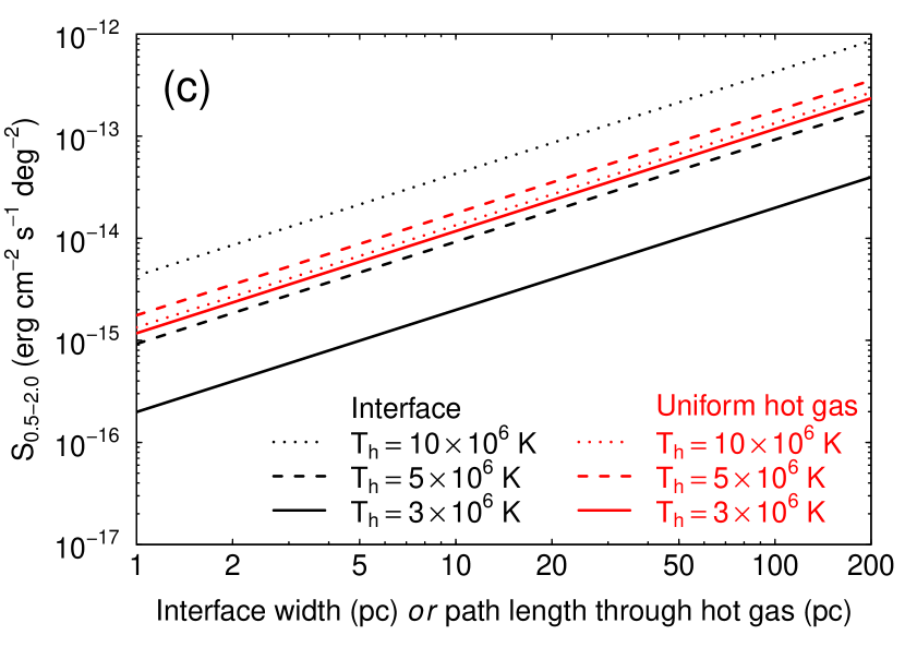
Figure 3.— (a) Temperature profiles for the interfaces between hot and cold gas described by Equation (2), with $T_{\mathrm{h}}=5\times 10^{6}~{}\mbox{K}$ and $T_{\mathrm{c}}=1\times 10^{4}~{}\mbox{K}$, for three different interface widths (solid: $w=0~{}\mbox{pc}$; dashed: $w=20~{}\mbox{pc}$; dotted: $w=100~{}\mbox{pc}$). (b) Profiles of the 0.5–2.0 keV emission for these model interfaces, where the plasma emissivity, $\varepsilon_{0.5-2.0}$, is a function of the temperature given by Equation (2), and the electron density, $n_{\mathrm{e}}$, is given by Equation (3). The plot shows profiles for the same values of $T_{\mathrm{h}}$ and $T_{\mathrm{c}}$ and for the same interface widths as in panel (a). (c): 0.5–2.0 keV surface brightnesses of these model interfaces (Equation (4); black curves) and of regions of uniform hot gas of temperature $T_{\mathrm{h}}$ (red curves), as functions of interface width, $w$, and of path length through the hot gas, respectively. In each case, results are shown for $T_{\mathrm{h}}=3\times 10^{6}$ (solid), $5\times 10^{6}$ (dashed), and $10\times 10^{6}~{}\mbox{K}$ (dotted), assuming $n_{\mathrm{e,h}}=10^{-3}~{}\mbox{cm}^{-3}$.

By integrating emission profiles like those shown in Figure 3(b) with respect to $x$, we can calculate the X-ray surface brightness of an interface described by Equations (2) and (3) as a function of interface width $w$,

$$S_{0.5-2.0}(w)=\frac{1}{4\pi}\int^{\infty}_{-\infty}\Big{\{} n_{\mathrm{e}}^{2}(x,w)\varepsilon_{0.5-2.0}(T[x,w])-$$

$$n_{\mathrm{e}}^{2}(x,0)\varepsilon_{0.5-2.0}(T[x,0])\Big{\}}dx$$ (4)

(for a sight line looking perpendicular to the interface). Note that, in the above expression, we subtract off the emission from a zero-width interface, so $S_{0.5-2.0}(w)$ is the increase in surface brightness due to increasing an interface’s width from zero to $w$. Note also that, since the integrand in Equation (4) is a function of $x/w$ (see Equations (2) and (3)), $S_{0.5-2.0}\propto w$. The surface brightnesses obtained from Equation (4) are shown by the black curves in Figure 3(c), for three different values of $T_{\mathrm{h}}$.

While increasing the widths of the interfaces would increase their surface brightness, in practice the increase in brightness cannot account for the discrepancy between the H12 predictions and the HS13 observations. This is because the emission from the diffuse hot gas tends to dominate over that from the interfaces between the hot gas and cooler gas, as we now demonstrate. The red curves in Figure 3 shows the surface brightnesses of uniform hot gas as functions of path length through the hot gas, for the same three values of $T_{\mathrm{h}}$ used for the black curves. For $T_{\mathrm{h}}\lesssim 5\times 10^{6}~{}\mbox{K}$, the surface brightness of an interface of a given width is less than the surface brightness of uniform hot gas of the same extent. As the regions of diffuse hot gas will likely be larger than the interfaces at their edges, the emission from the diffuse hot gas will tend to dominate. For example, consider a region of diffuse $5\times 10^{6}~{}\mbox{K}$ gas 500 pc in extent with zero-width interfaces at its edges. If thermal conduction were to increase the widths of those interfaces from zero to 100 pc, the total X-ray surface brightness would increase by only $\sim$20%. Therefore, increasing the widths of the interfaces in the model (by including thermal conduction) would not counteract the two-order-of-magnitude difference in brightness between the H12 predictions and the HS13 XMM-Newton observations.

6.3.2 Charge Exchange

The above discussion considered only emission resulting from collisional excitation of the gas in an interface. However, CX reactions between ions from the hot side of an interface and neutral H and He atoms from the cold side could also contribute to the emission. To estimate the importance of CX emission, we used Equation (1) from Lallement (2004). This gives the path length, $L_{\mathrm{CX}}$, through a hot gas for which the thermal emission from the hot gas is equal in brightness to the CX emission from the two interfaces at either end of the hot gas. Assuming the interfaces are observed at normal incidence, this path length is

$$L_{\mathrm{CX}}=0.06\frac{\epsilon\alpha n_{\mathrm{c}}V_{100}}{\chi n_{\mathrm{e}}^{2}}~{}\mbox{pc},$$ (5)

where $\epsilon$ is the ratio between the CX probability and the collisional ionization probability in the hot gas, $\alpha$ is the ratio of the global emissivity CX cross-section, $\Sigma$, to that assumed by Lallement (2004) ($\Sigma=6\times 10^{-19}~{}\mbox{keV}\ \mbox{cm}^{2}$, appropriate for solar wind CX emission in the 0.1–0.5 keV band), $\chi$ is the ratio of the hot gas emissivity to that assumed by Lallement ($5.8\times 10^{-14}~{}\mbox{keV}\ \mbox{cm}^{3}\ \mbox{s}^{-1}$), $n_{\mathrm{c}}$ and $n_{\mathrm{e}}$ are the number densities of the cold and hot gas, respectively, and $V_{100}$ is the relative speed of the ions and the neutrals in units of 100 km $\mbox{s}^{-1}$.

To estimate $L_{\mathrm{CX}}$, we assumed that the hot gas has a temperature of $3\times 10^{6}~{}\mbox{K}$, and used $\epsilon=0.2$ (from the $V=100~{}\mbox{km}\ \mbox{s}^{-1}$ curve in Figure 1 of Lallement 2004) and $\chi=0.17$ (the 0.5–2.0 keV emissivity of a $3\times 10^{6}~{}\mbox{K}$ plasma is $9.8\times 10^{-15}~{}\mbox{keV}\ \mbox{cm}^{3}\ \mbox{s}^{-1}$; Raymond & Smith 1977 and updates). In the absence of suitable CX emission data for the XMM-Newton band, we assumed $\alpha\sim 1$. We used a typical hot gas density of $5\times 10^{-5}~{}\mbox{cm}^{-3}$ (Table 1, column 5), and we assumed that the hot gas is in pressure equilibrium with cold gas with temperature $3\times 10^{4}~{}\mbox{K}$ (i.e., $n_{\mathrm{c}}=100n_{\mathrm{e}}$). Finally, we assumed that the relative motion of the ions and neutrals is dominated by thermal motion, and so used $V_{100}\sim 1$ (cf. the mean speed of oxygen ions in a $3\times 10^{6}~{}\mbox{K}$ plasma is 60 km $\mbox{s}^{-1}$).

Using the above values in Equation (5), we find $L_{\mathrm{CX}}\sim 140~{}\mbox{kpc}$, i.e., a region of hot ($T=3\times 10^{6}~{}\mbox{K}$, $n_{\mathrm{e}}=5\times 10^{-5}~{}\mbox{cm}^{-3}$) gas in pressure equilibrium with cooler ($3\times 10^{4}~{}\mbox{K}$) gas would have to be $\sim$140 kpc in extent in order for its 0.5–2.0 keV thermal emission to be as bright as the CX emission from the interfaces bounding the gas. In contrast, the path lengths through the hot gas in the H12 model are typically a few kiloparsecs (Table 1, column 7), implying that CX emission may be up to two orders of magnitude brighter than the thermal emission from the hot gas. It is therefore possible that CX emission could account for much of the shortfall between the current predictions from the H12 model and the observed halo surface brightness. However, from this simple estimate we cannot definitively conclude that most of the observed halo emission is due to CX—more detailed spectral calculations are needed to determine how much CX emission the H12 model produces. These calculations would have to be carried out for each hot-cold interface in the model individually, taking into account the temperature of the hot gas (which affects the populations of the ions undergoing CX reactions) and the densities of the hot and cold gas (which affect the overall brightness of the CX emission), and using CX cross-section and line yield data suitable for emission in the XMM-Newton band. Such calculations are beyond the scope of this paper.

If CX emission is indeed a major contributor to the observed halo X-ray emission, this would mean that the emission measure of the hot halo gas is smaller than previously thought (e.g., $\sim$$\mbox{(0.4--7)}\times 10^{-3}~{}\mbox{cm}^{-6}\ \mbox{pc}$; HS13). This would have important implications for the results of joint emission-absorption analyses of the halo, in which emission measurements are combined with ion column density measurements to infer the density and extent of the halo. In such an analysis, the extent of the hot halo scales as $N^{2}/\mathcal{E}$, where $N$ and $\mathcal{E}$ are the column density and emission measure of the hot gas, respectively. The density scales as $\mathcal{E}/N$, and so for a spherical halo, the gas mass scales as $\mathcal{E}/N\times(N^{2}/\mathcal{E})^{3}=N^{5}/\mathcal{E}^{2}$. Therefore, if the presence of CX means that the halo emission measure is overestimated, the extent and mass of the hot halo inferred from joint emission-absorption analyses will be underestimated.

6.4. Cosmic Ray Driving

In the H12 model, material is driven from the disk into the halo solely by the thermal pressure of SN-heated gas. However, CRs may also play an important role in driving outflows from galactic disks (Breitschwerdt et al., 1991). Everett et al. (2008) showed that a CR-driven galactic wind (modeled in one dimension) provided a better fit to the diffuse 3/4 keV emission observed toward the inner Galaxy ($-30\arcdeg<l<30\arcdeg$) than a static polytropic model. Salem & Bryan (2014), meanwhile, used three-dimensional AMR simulations to study CR-driven outflows. They showed that CR driving led to significant baryonic mass loss from the disk of their model galaxy, in contrast to a model without CR driving, in which there was no such mass loss. In addition, Salem & Bryan (2014) showed that including CR diffusion (as opposed to just having the CRs advect along with the gas flow) was important for driving the outflow from the disk.

In the context of the present study, including CR driving would be expected to result in more material being transported from the disk into the halo than in the H12 model, thus potentially increasing the halo’s X-ray surface brightness. However, the X-ray emission from such a CR-driven outflow also depends on its temperature structure. Booth et al. (2013) found that CR driving results in cooler outflows than pure thermal-pressure driving, but they chose a feedback implementation equivalent to the “energy only” runs in Agertz et al. (2013), which minimizes or eliminates hot gas production by SN explosions in dense gas (see Figure 6 in Agertz et al.). As a result, their prediction is only a lower limit on the true temperature. A model similar to the H12 model that incorporates CRs is currently under development (P. Girichidis et al. 2014, in preparation). The X-ray predictions from this new model will help determine the role of CR driving in supplying the hot halo gas observed in emission.

6.5. Role of an Extended Galactic Halo

Finally, we consider how an extended halo of hot gas ($\gtrsim$100 kpc in extent) might affect the H12 model predictions. The emission from the H12 model comes mostly from within a few kiloparsecs of the Galactic midplane. This is in part due to the low densities far above the disk in the model (typically $\lesssim$$3\times 10^{-5}~{}\mbox{cm}^{-3}$ above 10 kpc). In contrast, there is indirect evidence (from the lack of gas in satellite galaxies and the confinement of high-velocity clouds) for higher density halo gas far from the disk (Fang et al., 2013, and references therein). For example, a model of an extended non-isothermal halo in hydrostatic equilibrium with the Galaxy’s dark matter (Maller & Bullock, 2004), which is consistent with the observed X-ray emission and pulsar dispersion measure data, and with the aforementioned indirect evidence (Fang et al., 2013), has a density exceeding $10^{-4}~{}\mbox{cm}^{-3}$ out to $\sim$100 kpc (MB model in Figure 1 of Fang et al. 2013). Such extended hot halos are also predicted by disk galaxy formation models (e.g., Crain et al., 2010).

If the Milky Way’s extended halo consists of low-metallicity material accreted from the intergalactic medium, then in itself it would not be X-ray bright. However, from smoothed particle hydrodynamics (SPH) simulations of galaxy formation, Crain et al. (2013) found that the X-ray emission from their model galactic halos was produced by metals that were transported out of the ISM being collisionally excited by hot electrons in low-metallicity accreted gas. Hence, a hot, low-metallicity halo of accreted material could boost the X-ray emission from the fountains in the H12 model, by increasing the population of electrons available to excite the ions in the fountains. In addition, if there have been previous episodes of starburst activity in the Milky Way, these could have enriched the extended halo with metals, potentially making the extended halo intrinsically X-ray emissive. The arbitrary inflow at the boundaries of the JM06 model in fact raised the high-altitude densities above $10^{-4}~{}\mbox{cm}^{-3}$. As found in H10, this did indeed lead to X-ray surface brightnesses comparable to the observed values. If the extended halo is indeed intrinsically X-ray emissive, its emission would have to be added to that predicted by the H12 fountain model to get the total predicted halo emission. Note, however, that the observed halo emission is patchy, exhibiting large sight line-to-sight line variation (Yoshino et al. 2009; HS13). An extended halo model may have difficulty explaining this patchiness.

Predictions from hydrodynamical models of galaxy formation are needed to test the role played by an extended halo in producing the X-ray emission observed from the Milky Way’s halo. We plan to examine such predictions in a subsequent paper.

7. SUMMARY AND CONCLUSIONS

We have compared the X-ray emission predictions of a magnetohydrodynamical model of the SN-driven ISM (H12) with XMM-Newton measurements of the Galactic halo’s emission (HS13). This model significantly underpredicts the halo’s X-ray surface brightness (by two orders of magnitude, when we compare the medians of the predicted and observed values; Section 5). Including an interstellar magnetic field does not significantly affect these X-ray predictions.

We explored possible reasons for the discrepancy between the H12 model predictions and HS13’s XMM-Newton observations. Assuming CIE may in principle underestimate the emission from the H12 model halo, but in practice this is unlikely to have a significant effect (Section 6.2). We also found that the discrepancy could not be explained by the emission from interfaces in the H12 model being underestimated due to a lack of thermal conduction in the model (Section 6.3.1). However, CX emission from such interfaces (not included in the present emission model) could greatly increase the predicted X-ray surface brightness, though detailed spectral calculations are needed to confirm this (Section 6.3.2). (If CX emission is a major contributor to the observed halo emission, then the hot gas emission measure is less than previously thought, with the consequence that the path length and mass of the hot gas calculated from algebraic combinations of the emission measure and ion column density would be revised upwards.) In addition, CR driving of a wind could increase the amount of X-ray-emissive material in the halo (Section 6.4), and an extended hot halo of accreted material, while not intrinsically X-ray bright, may supply hot electrons that could increase the predicted X-ray emission from galactic fountains (Section 6.5).

In conclusion, the faintness of the H12 model relative to the observed surface brightness implies that thermal emission from classical galactic fountains is not a major source of the halo’s X-ray emission. This is in contrast to the conclusion of H10, which was based on the JM06 model (the X-ray predictions from which are now known to be incorrect). Our results indicate that additional physical processes need to be included in halo models. Two plausible possibilities are the effects of CR driving on the fountain, and extended hot halos from the galaxy formation process. In addition, CX may be an important contributor to the observed emission. Suitable X-ray predictions from CR-driven ISM models and galaxy formation models are needed to test the roles of galactic fountains and of accreted extragalactic material in explaining the observed X-ray emission from the Galactic halo.

References

- Agertz et al. (2013) Agertz, O., Kravtsov, A. V., Leitner, S. N., & Gnedin, N. Y. 2013, ApJ, 770, 25
- Begelman & McKee (1990) Begelman, M. C., & McKee, C. F. 1990, ApJ, 358, 375
- Booth et al. (2013) Booth, C. M., Agertz, O., Kravtsov, A. V., & Gnedin, N. Y. 2013, ApJL, 777, L16
- Bregman & Lloyd-Davies (2007) Bregman, J. N., & Lloyd-Davies, E. J. 2007, ApJ, 669, 990
- Breitschwerdt et al. (1991) Breitschwerdt, D., McKenzie, J. F., & Völk, H. J. 1991, A&A, 245, 79
- Breitschwerdt & Schmutzler (1994) Breitschwerdt, D., & Schmutzler, T. 1994, Nature, 371, 774
- Carter et al. (2011) Carter, J. A., Sembay, S., & Read, A. M. 2011, A&A, 527, A115
- Chen et al. (1997) Chen, L.-W., Fabian, A. C., & Gendreau, K. C. 1997, MNRAS, 285, 449
- Crain et al. (2010) Crain, R. A., McCarthy, I. G., Frenk, C. S., Theuns, T., & Schaye, J. 2010, MNRAS, 407, 1403
- Crain et al. (2013) Crain, R. A., McCarthy, I. G., Schaye, J., Theuns, T., & Frenk, C. S. 2013, MNRAS, 432, 3005
- Cravens et al. (2001) Cravens, T. E., Robertson, I. P., & Snowden, S. L. 2001, JGR, 106 (A11), 24883
- de Avillez & Breitschwerdt (2004) de Avillez, M. A., & Breitschwerdt, D. 2004, A&A, 425, 899
- de Avillez & Breitschwerdt (2012a) de Avillez, M. A., & Breitschwerdt, D. 2012a, ApJL, 756, L3
- de Avillez & Breitschwerdt (2012b) de Avillez, M. A., & Breitschwerdt, D. 2012b, ApJL, 761, L19
- Draine & Giuliani (1984) Draine, B. T., & Giuliani, Jr., J. L. 1984, ApJ, 281, 690
- Everett et al. (2008) Everett, J. E., Zweibel, E. G., Benjamin, R. A., et al. 2008, ApJ, 674, 258
- Ezoe et al. (2010) Ezoe, Y., Ebisawa, K., Yamasaki, N. Y., et al. 2010, PASJ, 62, 981
- Fang et al. (2013) Fang, T., Bullock, J., & Boylan-Kolchin, M. 2013, ApJ, 762, 20
- Fang et al. (2006) Fang, T., McKee, C. F., Canizares, C. R., & Wolfire, M. 2006, ApJ, 644, 174
- Fujimoto et al. (2007) Fujimoto, R., Mitsuda, K., McCammon, D., et al. 2007, PASJ, 59, S133
- Gupta et al. (2012) Gupta, A., Mathur, S., Krongold, Y., Nicastro, F., & Galeazzi, M. 2012, ApJL, 756, L8
- Hagihara et al. (2010) Hagihara, T., Yao, Y., Yamasaki, N. Y., et al. 2010, PASJ, 62, 723
- Henley & Shelton (2008) Henley, D. B., & Shelton, R. L. 2008, ApJ, 676, 335
- Henley & Shelton (2012) Henley, D. B., & Shelton, R. L. 2012, ApJS, 202, 14
- Henley & Shelton (2013) Henley, D. B., & Shelton, R. L. 2013, ApJ, 773, 92 (HS13)
- Henley & Shelton (2014) Henley, D. B., & Shelton, R. L. 2014, ApJ, 784, 54
- Henley et al. (2014) Henley, D. B., Shelton, R. L., Cumbee, R. S., & Stancil, P. C. 2014, ApJ, in press (arXiv:1411.5017)
- Henley et al. (2010) Henley, D. B., Shelton, R. L., Kwak, K., Joung, M. R., & Mac Low, M.-M. 2010, ApJ, 723, 935 (H10)
- Hickox & Markevitch (2006) Hickox, R. C., & Markevitch, M. 2006, ApJ, 645, 95
- Hill et al. (2012) Hill, A. S., Joung, M. R., Mac Low, M.-M., et al. 2012, ApJ, 750, 104 (H12; erratum 761, 189)
- Joung & Mac Low (2006) Joung, M. K. R., & Mac Low, M.-M. 2006, ApJ, 653, 1266 (JM06)
- Joung et al. (2012) Joung, M. R., Bryan, G. L., & Putman, M. E. 2012, ApJ, 745, 148
- Joung et al. (2009) Joung, M. R., Mac Low, M.-M., & Bryan, G. L. 2009, ApJ, 704, 137
- Kennicutt (1998) Kennicutt, Jr., R. C. 1998, ApJ, 498, 541
- Koutroumpa et al. (2007) Koutroumpa, D., Acero, F., Lallement, R., Ballet, J., & Kharchenko, V. 2007, A&A, 475, 901
- Kuntz & Snowden (2000) Kuntz, K. D., & Snowden, S. L. 2000, ApJ, 543, 195
- Lallement (2004) Lallement, R. 2004, A&A, 422, 391
- Mac Low et al. (2012) Mac Low, M.-M., Hill, A. S., Joung, M. R., et al. 2012, in ASP Conf. Ser. 459, Numerical Modeling of Space Plasma Flows (ASTRONUM 2011), ed. N. V. Pogorelov, J. A. Font, E. Audit, & G. P. Zank (San Francisco: ASP), 112
- Maller & Bullock (2004) Maller, A. H., & Bullock, J. S. 2004, MNRAS, 355, 694
- McKernan et al. (2004) McKernan, B., Yaqoob, T., & Reynolds, C. S. 2004, ApJ, 617, 232
- Moretti et al. (2003) Moretti, A., Campana, S., Lazzati, D., & Tagliaferri, G. 2003, ApJ, 588, 696
- Nicastro et al. (2002) Nicastro, F., Zezas, A., Drake, J., et al. 2002, ApJ, 573, 157
- R Development Core Team (2008) R Development Core Team. 2008, R: A Language and Environment for Statistical Computing, R Foundation for Statistical Computing, Vienna, Austria
- Rasmussen et al. (2003) Rasmussen, A., Kahn, S. M., & Paerels, F. 2003, in The IGM/Galaxy Connection. The Distribution of Baryons at , ed. J. L. Rosenberg & M. E. Putman (Dordrecht: Kluwer), 109
- Raymond & Smith (1977) Raymond, J. C., & Smith, B. W. 1977, ApJS, 35, 419
- Salem & Bryan (2014) Salem, M., & Bryan, G. L. 2014, MNRAS, 437, 3312
- Shapiro & Moore (1976) Shapiro, P. R., & Moore, R. T. 1976, ApJ, 207, 460
- Shelton (1998) Shelton, R. L. 1998, ApJ, 504, 785
- Smith et al. (2007) Smith, R. K., Bautz, M. W., Edgar, R. J., et al. 2007, PASJ, 59, S141
- Snowden et al. (2004) Snowden, S. L., Collier, M. R., & Kuntz, K. D. 2004, ApJ, 610, 1182
- Snowden et al. (2000) Snowden, S. L., Freyberg, M. J., Kuntz, K. D., & Sanders, W. T. 2000, ApJS, 128, 171
- Wargelin et al. (2004) Wargelin, B. J., Markevitch, M., Juda, M., et al. 2004, ApJ, 607, 596
- Yao & Wang (2007) Yao, Y., & Wang, Q. D. 2007, ApJ, 658, 1088
- Yao et al. (2009) Yao, Y., Wang, Q. D., Hagihara, T., et al. 2009, ApJ, 690, 143
- Yoshino et al. (2009) Yoshino, T., Mitsuda, K., Yamasaki, N. Y., et al. 2009, PASJ, 61, 805