Mapping and Matching Algorithms: Data Mining by Adaptive Graphs

Abstract

Assume we have two bijective functions $U(x)$ and $M(x)$ with $M(x)\neq U(x)$ for all $x$ and $M,N:\mathbb{N}\rightarrow\mathbb{N}$ . Every day and in different locations, we see the different results of $U$ and $M$ without seeing $x$. We are not assured about the time stamp nor the order within the day but at least the location is fully defined. We want to find the matching between $U(x)$ and $M(x)$ (i.e., we will not know $x$). We formulate this problem as an adaptive graph mining: we develop the theory, the solution, and the implementation. This work stems from a practical problem thus our definitions. The solution is simple, clear, and the implementation parallel and efficient. In our experience, the problem and the solution are novel and we want to share our finding.

1 Introduction

Let start by introducing the problem by its practical case. We are traveling with our smart phone. We take a taxi and go to the airport. We surf using our data plan. We arrive at the airport and we connected to the local WiFi, we surf. Before boarding we turn off our phone. We land and the previous process restarts. During our surfing, our phone will be identified by a unique number as a function of the device and application (i.e., UUID). While we are using the WiFi, our device will have also a MAC address and IP. If we have the distinct set of MACs and UUIDs, can we find the match: what UUID is associated with the MAC?

If we identify our phone as $x$, we have two deterministic functions: function $U(x,t,\ell)$ with location $\ell$ and time $t$ that identifies our unique device, and function $M(x,t,\ell)$ with location and time that identifies the MAC. We have only a sample in time of $U(x,t,\ell)$ and a sample by location of $M$. In practice, We may not gain $U(x)$ and $M(x)$ at the same time but in a reasonable interval of time, say one day: for example, at a specific airport and date (day) we may have either one but not both with no specific time information beside the day. Also, given $x$ we may have $S=U(x,t_{i},\ell_{j})$, that is $U(x)$ is not unique and it may the composition of a set of exclusive functions $U_{i}(x)$ but when possible we enforce a deterministic and unique result.

The problem boils down as to answer the following question: If we are observing the output of $U$ and $M$, can we guess $x$, which is associated to $U(x)$ and $M(x)$?

We define an airport as $L_{i}$ with $i\in[0,N-1]$. There are $N$ airports and we enumerate them. We describe the first day we observe events simply as $t_{0}$. Thus $t_{1}$ is the second day: this will imply that day $t_{i}$ precedes $t_{i+1}$.

Let us start considering the first day $t_{0}$. For every $L_{i}$ there is a set of associated MAC address, we identify this set as $M_{t_{0}}^{L_{i}}$. Also, we determine the users in one mile radius from $L_{i}$: We identify this set as $S_{t_{0}}^{L_{i}}$.

(1.1) $$S_{t_{0}}^{L_{i}}=\{u:dist(u,L_{i})<1\mbox{ at time }t_{0}\}$$

The user set $S_{t_{j}}^{L_{i}}$ is not complete because we have only a sample of the available impressions: we sample in time the values of $U(x,t,\ell)$, we cannot keep an ordered time sequence beside a day granularity, and by construction we may cover only a small area of the airport $L_{i}$.

In practice, we associate $\langle S_{t_{0}}^{L_{i}}:M_{t_{0}}^{L_{i}}\rangle$, the departing addresses to the departing users. This is the mapping we would like to refine as much as possible, until we can have a one-to-one matching. That is, we can infer the hidden $x$ that determines the unique mapping between $U(x)$ and $M(x)$. These same users are landing to different $L_{j}$ with $i\neq j$ and thus different addresses $M_{t_{0}}^{L_{j}}$ and $M_{t_{1}}^{L_{j}}$ may be given.

Every mapping $\langle S_{t_{j}}^{L_{i}}:M_{t_{j}}^{L_{i}}\rangle$ describes a graph, a fully connected bipartite graph. We need to combine all mappings as above in order to achieve our goal. This is an adaptive graph algorithm: we build a graph step by step, day by day. We check whether mappings in different graphs have intersection and we can split the graph by cutting edges.

The final goal is to grind these mappings into matches where one user is associate to one MAC or at least to the finest refinement possible. In the following, we formulate our solution using the same notations, we present our algorithm, a few simplifications, and our results.

2 The algorithm

Consider the mappings for the first day: $\langle S_{t_{0}}^{L_{i}}:M_{t_{0}}^{L_{i}}\rangle$. These can be considered as the departing addresses for the departing users. The users departing from $L_{i}$ can be the user landing at $L_{j}$ with $j\neq i$. If there is intersection between addresses we could refine the mapping:

(2.2) $$\begin{split}{\langle S_{t_{0}}^{L_{i}}:M_{t_{0}}^{L_{i}}\rangle}=&\langle S_{t_{0}}^{L_{i}}\smallsetminus\Big{(}\bigcup_{n=0,1}^{i\neq j}S_{t_{n}}^{L_{j}}\Big{)}:M_{t_{0}}^{L_{i}}\smallsetminus\Big{(}\bigcup_{n=0,1}^{i\neq j}M_{t_{n}}^{L_{j}}\Big{)}\rangle+\\ &\sum_{j\neq i}\langle S_{t_{0}}^{L_{i}}\cap\big{(}\bigcup_{n=0,1}S_{t_{n}}^{L_{j}}\big{)}:M_{t_{0}}^{L_{i}}\cap\big{(}\bigcup_{n=0,1}M_{t_{n}}^{L_{j}}\big{)}\rangle\\ \end{split}$$

Here the $+$ operation is the disjoint concatenation of mappings binding fewer elements and refining them towards matches. Our interpretation of Equation 2.2 follows: if there is any landing information the mapping between departing users and departing address, then we can refined the mapping into two major components.

(2.3) $$\langle\dot{S}_{t_{0}}^{L_{i}}:\dot{M}^{L_{i}}_{t_{0}}\rangle\equiv\langle S_{t_{0}}^{L_{i}}\smallsetminus\Big{(}\bigcup_{n=0,1}^{i\neq j}S_{t_{n}}^{L_{j}}\Big{)}:M_{t_{0}}^{L_{i}}\smallsetminus\Big{(}\bigcup_{n=0,1}^{i\neq j}M_{t_{n}}^{L_{j}}\Big{)}\rangle$$

Equation 2.3 and 2.2.(part one) refer to the departing users without landing information.

(2.4) $$\sum_{j}\langle S^{L_{i}\rightarrow L_{j}}_{t_{0}}:M^{L_{i}\rightarrow L_{j}}_{t_{0}}\rangle\equiv\sum_{j\neq i}\langle S_{t_{0}}^{L_{i}}\cap\Big{(}\bigcup_{n=0}^{1}S_{t_{n}}^{L_{j}}\Big{)}:M_{t_{0}}^{L_{i}}\cap\Big{(}\bigcup_{n=0}^{1}M_{t_{n}}^{L_{j}}\Big{)}\rangle$$

If there is an intersection between departing and landing users, we refine the mapping with the intersection of the departing and landing addresses. The locations are disjoint, very likely a user will be only at two locations in two days and thus $S_{t_{0}}^{L_{i}}\cap\big{(}\cup_{n=0,1}S_{t_{n}}^{L_{j}}\big{)}$ will be true only for one $j$, then the mappings are disjoint. Because we are considering two consecutive days we may have to combine two or more mappings one step further. Let us introduce the product of mappings.

By definition, if we have a $\langle A:M\rangle$ any user in $A$ can be mapped to any address in $M$. As a graph, this represents a bipartite fully-connected graph. If we have another mapping $\langle B:N\rangle$ and there is an intersection between addresses, then we know that the same users should be in both $A$ and $B$. After all the address is unique to the device. It makes sense to take the intersection of users as well. In practice, we assume users will have likely or consistently the same user identification number. This will refine the mapping reducing the size of the three resulting mappings:

(2.5) $$\begin{split}\langle A:M\rangle*\langle B:N\rangle=&\langle A\smallsetminus B:M\smallsetminus N\rangle+\\ &\langle A\cap B:M\cap N\rangle+\\ &\langle B\smallsetminus A:N\smallsetminus M\rangle\\ \end{split}$$

We use the $*$ operator to represent this operation. In combination with $+$ operator, our algorithm will be based an algebra. If there is no intersection, there is no refinement and $\langle A:M\rangle*\langle B:N\rangle=\langle A:M\rangle+\langle B:N\rangle$.

If there are only two mappings the product is intuitive and the final result is a disjoint mapping. Let us consider two mappings composed by disjoint simpler mappings and their products

(2.6) $${\cal P}=\Big{(}\sum_{j=0}^{K-1}w_{j}\Big{)}*\Big{(}\sum_{i=0}^{L-1}v_{i}\Big{)}$$

where $w_{j}=\langle A_{j}:M_{j}\rangle$ and $v_{i}=\langle B_{i}:N_{i}\rangle$. We will abuse the set notation a little here:

(2.7) $$\begin{split}{\cal P}=&\sum_{j=0}^{K-1}\Big{(}\sum_{i=0}^{L-1}w_{j}\smallsetminus v_{i}\Big{)}+\\ &\sum_{j=0}^{K-1}\sum_{i=0}^{L-1}w_{j}\cap v_{i}+\\ &\sum_{i=0}^{L-1}\Big{(}\sum_{j=0}^{K-1}v_{i}\smallsetminus w_{j}\Big{)}\\ \end{split}$$

We notice that the sum $\sum_{i=0}^{L-1}w_{j}\smallsetminus v_{i}\equiv\sum_{i=0}^{L-1}\langle A_{j}\smallsetminus B_{i}:M_{j}\smallsetminus N_{i}\rangle$ is not disjoint because every term has in common the mapping:

$$w_{j}\smallsetminus(\sum_{i=0}^{L-1}v_{i})\equiv\langle A_{j}\smallsetminus\cup_{i=0}^{L-1}B_{i}:M_{j}\smallsetminus\cup_{i=0}^{L-1}M_{i}\rangle$$

also $w_{j}\smallsetminus v_{0}$ and $w_{j}\smallsetminus v_{1}$ have in common the one above and $\sum_{i=2}^{L-1}w_{j}\cap v_{i}$, which are already included in the second term in Equation 2.7. Thus the first term in Equation 2.7 becomes basically $\sum_{j=0}^{K-1}w_{j}\smallsetminus(\sum_{i=0}^{L-1}v_{i})$.

(2.8) $$\begin{split}{\cal P}=&\sum_{j=0}^{K-1}w_{j}\smallsetminus(\sum_{i=0}^{L-1}v_{i})+\\ &\sum_{j=0}^{K-1}\sum_{i=0}^{L-1}w_{j}\cap v_{i}+\\ &\sum_{i=0}^{L-1}v_{i}\smallsetminus(\sum_{j=0}^{K-1}w_{i})\\ \end{split}$$

Equation 2.8 represents a disjoint mapping.

Let us return to Equation 2.2.(part two) and 2.4 especially how to combine the terms that have intersection: we can imagine that the index $j$ infers an order for the components: the destination $L_{0}$, $L_{1}$, …, and $L_{N-1}$. At the end of the first day $t_{0}$ we can summarize our knowledge as

(2.9) $$\begin{split}D_{t_{0}}=&\sum_{i=0}^{N-1}\langle\dot{S}_{t_{0}}^{L_{i}}:\dot{M}^{L_{i}}_{t_{0}}\rangle+\\ &\sum_{j=0}^{N-1}\prod_{i=0}^{N-1}\langle S^{L_{i}\rightarrow L_{j}}_{t_{0}}:M^{L_{i}\rightarrow L_{j}}_{t_{0}}\rangle\end{split}$$

For the refinement in Equation 2.9, we have a disjoint set of mappings. Now we must combine them. The first term in Equation 2.2.(part one) presents disjoint mappings and thus can be just added in Equation 2.9. The second term is a little trickier. We see it as the intersection of mappings that have common users and thus narrowing the mapping size. The second should reduce to a perfect matching and when it does we can remove the users and put them aside.

Now let us consider the second day $t_{1}$. Let us compute $D_{t_{1}}$ independently from the previous step. Then we join the two steps by checking users intersections and refining the mappings: for each mapping in $D_{t_{1}}$ we can make a product/intersection of each mapping in $D_{t_{0}}$ and thus:

$$D_{t_{1}}=D_{t_{1}}*D_{t_{0}}$$

See the symmetric property of the product. Before any product or update, the terms are a list of disjoint mappings. The product is meant to combine mappings that have common addresses so that to refine the mappings into matches.

We should keep an order during the concatenation, for example:

(2.10) $$\begin{split}D_{t_{k+1}}=&\\ D_{t_{k+1}}*D_{t_{k}}=&\Big{(}\sum_{i=0}^{N-1}\langle\dot{S}_{t_{k}}^{L_{i}}:\dot{M}^{L_{i}}_{t_{k}}\rangle+\sum_{j=0}^{N-1}\prod_{i=0}^{N-1}\langle S^{L_{i}\rightarrow L_{j}}_{t_{k}}:M^{L_{i}\rightarrow L_{j}}_{t_{k}}\rangle\Big{)}*\\ &\Big{(}\sum_{i=0}^{N-1}\langle\dot{S}_{t_{k+1}}^{L_{i}}:\dot{M}^{L_{i}}_{t_{k+1}}\rangle+\sum_{j=0}^{N-1}\prod_{i=0}^{N-1}\langle S^{L_{i}\rightarrow L_{j}}_{t_{k+1}}:M^{L_{i}\rightarrow L_{j}}_{t_{k+1}}\rangle\Big{)}\\ \end{split}$$

3 A Study in Parallelism

The daily mappings $\langle S_{t_{i}}^{L_{i}}:M_{t_{0}}^{L_{i}}\rangle$ requires the data from two consecutive days: $t_{i}$ and $t_{i+1}$. The first parallel computation is based on the split of the interval of time into smaller and consecutive intervals: two week interval each, say. We compute each two-week interval in parallel. This is an embarrassing parallelism.

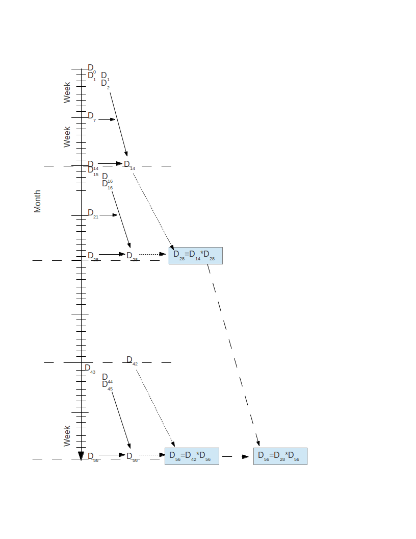
Figure 1: Decomposition of the computation

The total interval of time is composed of six months of data, we actually split the computation into up to 15 independent computations. Each $D_{t_{j}}$ is composed by a set of matches and mappings. We take the list of $D_{t_{j}}$ and compute consecutive-pair products as a binary tree.

Obviously, the last computation in the binary tree is a single product and it seems that there is no parallelism to exploit. Take the example in Figure 1. The final product $D_{56}=D_{28}*D_{56}$ will require at least as much as the sum of the previous computations: $O(D_{14}*D_{28})+O(D_{42}*D_{56})$, which does not seem parallel friendly.

In practice, as we go up in the tree, we loose explicit parallelism but we can exploit the same amount of parallelism in the product. Thus, we can keep the same level of parallelism throughout the computation and thus efficient use of any architecture.

The product becomes more complex as we go up. In fact, the product has to explore a Cartesian product of the operand mappings (graphs). We explore if there are edges across the operands and this is why we use the term adaptive for the graph we explore and build.

4 The Implementation

# R implementation
product <- function(D0,D1,P=2) {
  if (length(D0) ==0 && length(D1)==0)     {  R = list()   }
  else if ((is.null(D0) || length(D0) ==0) && length(D1)>0) {  R =  D1      }
  else if (length(D0) >0 && (is.null(D1) || length(D1)==0)) {  R =  D0      }
  else {
      L = group2(1:length(D0),length(D0)/P)
      ii <- function(K) {
          i=0; R = list(); D = list(’S’=c(),’M’=c())
          for (k in K) {
              l = i
              Q = list(’S’=c(),’M’=c())
              for (j in 1:length(D1)) {
                  S = intersect(D0[[k]]$S,D1[[j]]$S)
                  M = intersect(D0[[k]]$M,D1[[j]]$M)
                  if (length(M)>0 && length(S)>0) {
                      i = i +1;  R[[i]] =list(’S’=S,’M’=M)
                      Q$M = union(Q$M,M)
                      Q$S = union(Q$S,S)
                  }
              }
              if (i>l) {
                  S = setdiff(D0[[k]]$S,Q$S)
                  M = setdiff(D0[[k]]$M,Q$M)
                  if (length(M)>0 && length(S)>0) {
                      i = i +1;  R[[i]] =list(’S’=S,’M’=M)
                  }
                  D$M = union(D$M,Q$M)
                  D$S = union(D$S,Q$S)
              } else {
                  i = i +1;  R[[i]] = D0[[k]]
              }
          }
          list("R"=R, "D" = D, "disjoint"=(i==0))
      }

      RT = mclapply(L,ii,mc.preschedule=TRUE,mc.cores=P)

      R = list();   D = list(’S’=c(),’M’=c());      disjoint = TRUE;   i=0
      for (rt in RT) {
          if (length(rt)>0) {
              for (r in rt$R) {
                  i = i +1;  R[[i]] = r
              }
              disjoint = disjoint && rt$disjoint
              D$M = union(D$M,rt$D$M)
              D$S = union(D$S,rt$D$S)
          }
      }
      if (disjoint) {
          for (k in 1:length(D1)) {
              i = i +1;  R[[i]] = D1[[k]]
          }
      } else {
          for (k in 1:length(D1)) {
              S = setdiff(D1[[k]]$S,D$S)
              M = setdiff(D1[[k]]$M,D$M)
              if (length(M)>0 && length(S)>0) {
                  i = i +1;  R[[i]] = list(’S’=S,’M’=M)
              }
          }
      }
      R
  }
}

The product is the core of the whole computation. The software came after the formal solution was found. The first implementation was verbatim from Equation 2.8. This was a good starting point. There are actually a few drawbacks: First, the intersections are sparse and not balanced; that is, there may be intersection between $S_{i}$ but not in between $M_{i}$ or viceversa. This means that the computation $\sum_{j}\sum_{i}w_{j}v_{i}$ will spend quite some work finding empty intersections and this information is not used for the other terms. Abusing a little the notation, we can rewrite the computation in such a way that we avoid the graphs union computations by computing the intersection first and reuse it:

(4.11) $$\begin{split}T=&\emptyset\\ {\cal P}=&\sum_{\ell=+\frac{K}{P}}\Big{(}\big{(}T{\cup=}W=\sum_{j=0}^{\frac{K}{P}}\sum_{i=0}^{L-1}w_{j+\ell}*v_{i}\big{)}+\sum_{j=0}^{\frac{K}{P}}w_{j+\ell}\smallsetminus W\Big{)}+\\ &\sum_{i=0}^{L-1}v_{i}\smallsetminus T\\ \end{split}$$

Above, we present the implementation in R of the product. The operand $D0$ is the mappings at time $t_{i}$ ($t_{0}$) and the operand $D1$ is the mappings at time $t_{i+1}$ ($t_{1}$).

The implementation has an important difference from Equation 2.8 and the intent in Equation 4.11, the intersection has to be non empty for both $S$ and $M$ to be recorded and used (in the following set difference computation). If we could apply equation 2.8, the final product will be the composition of disjoint terms. The implementation of Equation 4.11 does not assure that the final product has disjoint terms and actually it may allow identical terms to appear, thanks to the symmetric nature or the graph. Our implementation allows a minimum and consistent computation: equal terms are removed and no-disjoint terms involving perfect matches are simplified.

As we can see, the product explores all pairs to find intersections, a square effect on the computational complexity. Our implementation choice is based on reducing the complexity even though by a constant.

5 The Case Study

Due to the proprietary nature of the data, we cannot share the set itself and a few of its details. However, we share the code verbatim because of its simplicity (and will share the code upon request).

We observed about six airports for about six months. We observed about five hundred thousand unique MACs that appear more than once (if there is only one appearance, there is very little signal and a matching will be possible only if we match all other MACs, which is unlikely).

We observed nine million unique users collected in a radius of one mile from the airports requested center of interest and they appeared more than two times during the entire period. On average, we have 2.5 million unique users and ten thousand unique MACs per day.

We build the mappings using two different granularities. See Figure 1. We use a granularity of two and four weeks to start the computation. This is to cope with the randomness of the user observation: We can only obtain a sample of the users UUID and their appearance or their lack affect the matches and their products. Also the asymmetric nature of the product implementation exemplified of Equation 4.11 will make the resulting graphs different. Otherwise, the graphs should be completely deterministic, consistently built and eventually identical.

Table 1: Two/four-week mapping graph (above) and user/mac distribution (below)

weeks	matches	mappings	users covered	macs coverage
2	30667	130304	23448155	689828
4	33912	126650	24153536	686038

Table 2: Ratio user/mac distribution

weeks	Min.	1st Qu.	Median	Mean	3rd Qu.	Max.
2	0.007	3.000	8.000	80.990	30.000	28690.000
4	0.012	3.000	8.000	87.940	32.000	27440.000

The computation time also may differ because of the different sparsity of the mappings and their combinations. We present the results separately and we conclude this section with a few considerations.

5.1 The two and four week graphs

The process follows the one presented in Figure 1, we start building day-by-day graph up to two/four weeks. Then, we build the full graph.

Using the same number of resources, 16 cores for each computation, the four week graph is a little faster (i.e., 2 hrs faster for a 4 days computation from end-to-end), provides more matches, fewer mappings but more redundancy. Notice that the two-week graph exploits more parallelism and it will be faster if more resource could be used at the beginning of the process.

If we take a graph and we compute the ratio of the users number over the MACs number in each mapping, we can summarize the graphs using their distributions. We summarize their distribution in Table 2. In practice, the two-week graph has fewer matches but the mappings tend to be more refined than the mappings in the four-week graph, Table 2.

We have not tried to combine the results (four and two weeks); it is possible to take the graphs combine the matches and then compute the product of the mappings. This is left as future investigation.

5.2 Considerations

The problem formulation and its notations were used to write a first implementation: the first prototype was applied to a small graph after a few weeks. The choice to write the solution in R was for the ease in connecting to different databases where the data were available. The simple semantic of the language fit the original formulation well.

As we increased the size of the graph, we decided to keep the original solution, exploit the R parallelism, and to beef up the hardware (from 8-cores 32 GB machine to 32-cores 128GB). However, the square complexity (i.e., O($N^{2}$) nodes of the graph) forced us to tune the code and to relax the computation. We had to exploit parallelism in a way that it is not natural to R.

We would suggest to chose a different environment or language to exploit parallelism at loop level.

6 Conclusion

To the best of our knowledge, the problem is novel because the refinement of the mappings requires the intersection of two different sets. There is no truth given a priori and thus there is no learning. This is an example of graph mining. To the best of our knowledge, our solution is novel as well.

We provide a formal definition of the problem and its solution in order to start a conversation. The formal statement actually have been driving our problem presentation and solution. The desire of a well defined formalism helped us freeing ideas by means of no ambiguity and dangerous and misplaced intuitions.

As result, we have a solution that balances parallelism in an elegant fashion as it unfolds during the computation. This parallelism is not common and we wanted to share its application. This, in itself, could be attractive to others.